Implementability of distributed systems described with scenarios

(1)

HAL Id: tel-00919684

https://tel.archives-ouvertes.fr/tel-00919684

Submitted on 17 Dec 2013

HAL is a multi-disciplinary open access archive for the deposit and dissemination of sci-entific research documents, whether they are pub-lished or not. The documents may come from

L’archive ouverte pluridisciplinaire HAL, est destinée au dépôt et à la diffusion de documents scientifiques de niveau recherche, publiés ou non, émanant des établissements d’enseignement et de

Implementability of distributed systems described with

scenarios

Rouwaida Abdallah

To cite this version:

Rouwaida Abdallah. Implementability of distributed systems described with scenarios. Other [cs.OH]. École normale supérieure de Cachan - ENS Cachan, 2013. English. �NNT : 2013DENS0027�. �tel-00919684�

(2)

Implementability of distributed systems described

with scenarios

by c

¥Rouwaida ABDALLAH

A Thesis submitted to the School of Graduate Studies in partial fulfillment of the requirements for the degree of

PHD in Computer Science Ecole Normale Superieure de cachan

ENS-cachan

July 2013

(3)

(4)

Abstract

Distributed systems lie at the heart of many modern applications (social networks, web services, etc.). However, developers face many challenges in implementing dis-tributed systems. The major one we focus on is avoiding the erroneous behaviors, that do not appear in the requirements of the distributed system, and that are caused by the concurrency between the entities of this system.

The automatic code generation from requirements of distributed systems remains an old dream. In this thesis, we consider the automatic generation of a skeleton of code covering the interactions between the entities of a distributed system. This allows us to avoid the erroneous behaviors caused by the concurrency. Then, in a later step, this skeleton can be completed by adding and debugging the code that describes the local actions happening on each entity independently from its interactions with the other entities.

The automatic generation that we consider is from a scenario-based specification that formally describes the interactions within informal requirements of a distributed system. We choose High-level Message Sequence Charts (HMSCs for short) as a scenario-based specification for the many advantages that they present: namely the clear graphical and textual representations, and the formal semantics. The code

(5)

gen-eration from HMSCs requires an intermediate step which is their transformation into an abstract machine model that describes the local views of the interactions by each entity (A machine representing an entity defines sequences of messages sending and reception). This transformation is called "synthesis". Then, from the abstract ma-chine model, the skeleton’s code generation becomes an easy task.

A very intuitive abstract machine model for the synthesis of HMSCs is the Com-municating Finite State Machine (CFSMs for short). However, the synthesis from HMSCs into CFSMs may produce programs with more behaviors than described in the specifications in general. We thus restrict then our specifications to a sub-class of HMSCs named "local HMSC". We show that for any local HMSC, behaviors can be preserved by addition of communication controllers that intercept messages to add stamping information before resending them.

We then propose a new technique that we named "localization" to transform an ar-bitrary HMSC specification into a local HMSC, hence allowing correct synthesis. We show that this transformation can be automated as a constraint optimization problem. The impact of modifications brought to the original specification can be minimized with respect to a cost function.

Finally, we have implemented the synthesis and the localization approaches into an existing tool named SOFAT. We have, in addition, implemented to SOFAT the au-tomatic code generation of a Promela code and a JAVA code for REST based web services from HMSCs.

(6)

Thank you

(11)

Chapter 1 Introduction

1.1 Context

A distributed system consists of a collection of autonomous entities (i.e., computers, processes), that are connected through a network which enables them to communicate and to share common resources. From 1945 until mid 80’s, computers were large and expensive: A mainframe used to cost millions of dollars; even minicomputers used to cost at least tens of thousands of dollars each. That is why, most organizations only had a handful of computers. Furthermore, these computers operated indepen-dently because there was no way to connect them. Since the mid 80’s, the advances in technology, namely the development of powerful microprocessors and the invention of high-speed networks, have begun to change that reality [80]. Since, distributed systems have become widely used in many applications that range from television sets and train signaling systems to e-commerce and stand-alone PC-based software applications. These days distributed systems have become a need, as many recent ap-plications are by nature distributed (bank teller machines, airline reservations, ticket purchasing, communication applications, social networks, etc.).

1.2 Motivation

Nowadays, distributed systems are everywhere and there is a concrete need for imple-menting functional, usable, and high-performance distributed systems. It is therefore

(12)

important for the developers to have an understanding of the requirements of the sys-tem and the problems that may occur. Actually, the various entities in a distributed system can operate concurrently and possibly autonomously and this concurrency gives rise to a number of well-studied problems: Processes may use old data; they can make inconsistent updates; the order of updates may or may not matter; the system might deadlock; the data in different systems might never converge to consistent val-ues; etc [44]. Several of these problems come from the erroneous behaviors that occur in the system and that were not described in the requirements. Actually, it is not an easy task to correctly move from requirements towards a distributed implementation while preserving the set of required behaviors for the entities of the distributed system. We have mainly two distinct approaches to go from requirements to implementation: On one hand, developers consider generally to go directly from informal requirements to implementation. Prototyping and testing remain the principal methods for develop-ers for exploring designs and validating implementations. Methods like the V-Model software development process, presented in Figure 1.1, may be used in the develop-ment of distributed system. The V-Model consists respectively in defining a design that describes the requirements of the system, implementing the corresponding code, and finally testing this code. The V-Model software development process might be repeated several times while still finding modifications to do. Such methods are ex-pensive in terms of time and money (the code might be tested and modified several times) and provide only partial coverage of the range of behaviors that a piece of software may exhibit (it is hard to cover and test all the behaviors that may occur on the system, and when the set of behaviors is infinite testing all of them is impossible). On the other hand, the second approach, which is the one that we consider in this the-sis, is the implementation based on the use of scenario-based specifications. Scenario-based specifications present the abstract descriptions of the interactions between the entities of the system. They have become popular as a powerful means of communica-tion for system requirements due to their simplicity and expressive power [40]. Some scenario-based specifications have solid mathematical foundations that can be used to support rigorous analysis and mechanical verification of properties. They allow verifications of system requirements at early stages before the implementation of the code of the system. Their use ranges from requirements engineering [40] and formal specifications [75] to code synthesis [3] and test case specification and generation (e.g. [32]). Furthermore, scenario-based specifications are used to move from requirements towards a skeleton of an implementation for distributed systems and thus to facilitate

(13)

Figure 1.1: The V life cycle model in software development

their construction: Scenario-based specifications mainly describe the interactions be-tween the entities of the distributed system and not the detailed behaviors occurring locally on each entity. Then, the implementation of scenarios results in a skeleton of code that presents the interactions within the distributed system described in the requirements. The rest of the code, that describes the local behaviors for each entity, can then be debugged and added to the skeleton of code to get the complete imple-mentation of the distributed system. Furthermore, the automatic generation of this skeleton of code is very important and offers many advantages:

• The errors that might be induced by developers’ implementations are avoided, as this transformation from scenario-based specification into a code is an error-prone task. The correct generation of the skeleton helps the developers to avoid the problems caused by the concurrency in distributed systems.

• Skeleton’s code generation is time saving and can lead to a relatively fast gen-eration of prototype and test cases software.

• The high redundancy in distributed systems’ code, makes this automatic gener-ation a desirable goal. It will save time needed for writing similar and redundant code.

In this thesis, we are interested in producing a reliable implementation for distributed systems. We will consider a scenario-based specifications approach and our main target is to propose a method that transforms requirements into a skeleton of code that guarantees correct interactions behaviors in a distributed system.

(14)

1.3 The synthesis problem

To proceed the skeleton’s code generation from a scenario-based specification, we have an intermediate step. This step transforms the scenario-based specification, which is a high-level specification that describes the behaviors of the system from a global point of view, into an abstract machine model that describes the local views (the commu-nicating machines, which define sequences of messages sendings and receptions) that is consistent with the original specification. Then, from the abstract machine model the skeleton’s code generation becomes an easy task. This transformation from a high-level specification to an abstract machine model is called the synthesis.

This thesis addresses the automatic synthesis problem in the context of distributed applications running on networks of computers, and more precisely correct synthesis algorithms. Synthesis is correct when the abstract machine model preserves the be-haviors described in the high-level specification.

In the literature, many different definitions of scenario-based specifications can be found [23, 19, 45, 50]. There are significant differences in terms of syntax, features, semantics, etc. (a more detailed presentation and comparison of scenarios is pre-sented in chapter 2). Sequence charts are one of the approaches to describe scenarios. Sequence charts have been used to describe system behaviors for some time before the International Telecommunications Union (ITU), has undertaken their standard-ization process. This has resulted in a language called Message Sequence Charts (MSCs). MSCs have undergone several revisions since their first version, the latest one being in 2011 [1].

MSCs are particularly useful in the early stages of system development; they allow describing the communications of a system and can be used to find design errors. First, the graphical representation of MSCs is one of the reasons for their popularity. It makes MSCs intuitively comprehensible and easy to learn and there is no need to have a mathematical background to start using this notation. Furthermore, MSCs have a textual representation that was originally intended for exchanging MSCs be-tween tools. Last but not least, MSCs also have a formal semantics, which allows them to be used for various analysis purposes. Since MSCs are used at a very early stage of design, any error revealed during their analysis yields a high pay-off. This has already motivated the development of algorithms for a variety of analyses includ-ing the presence of a race condition in an MSC [9], model checkinclud-ing [10], pattern

(15)

matching [69], detection of non-local choices [15, 31], deadlocks, livelocks, and many more (for more details see e.g. [24]).

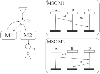
Figure 1.2: Example of MSCs: two bMSCs M1 and M2 and one HMSC H

MSCs are composed of several specification layers. At the lowest level, basic MSCs (bMSCs for short) defining finite specifications of interactions among processes. For instance, Figure 1.2 shows two examples of bMSCs M1 and M2, where two processes

A and B interchange messages: In bMSC M1, the process A sends a message m1

to the process B then B sends a message m2 to A. M2 presents another scenario

where B sends the message m3 to A then A sends m4 to B. However, the real sys-tems are often very complex. MSC specification allows addressing the complexity of distributed systems by composing bMSCs with several means. High-level MSCs (HMSCs for short) describe the composition of bMSCs in a clear and attractive way, which makes them the most used composition mechanism. For instance, Figure 1.2 shows an example of an HMSC H, that composes the two bMSCs M1 and M2. It

describes an alternative between the bMSC M1 or M2. The whole MSC formalism

will be described later in chapter 2.

In this thesis, we will consider the synthesis of HMSCs. A very natural way to syn-thesize abstract machine models from HMSCs is by projection (see chapter 3). The principle of projection is to copy the original behaviors specified in the HMSC spec-ification on each process in the distributed system, and to remove the part of the behaviors that do not belong to this considered process.

(16)

A very intuitive abstract machine model for the projection of HMSCs is the Commu-nicating Finite State Machine [17] (CFSMs for short). This model presents several advantages; it allows the definition of concurrent components exchanging messages asynchronously through FIFO channels. This well-known formalism is easily imple-mentable on many distributed platforms built on top of standard communication protocols (TCP, REST, ...).

Unfortunately, all the global coordination expressed by HMSCs cannot always be translated to CFSMs in the synthesis by projection algorithm. Consequently, some HMSC specifications may not be implementable as CFSMs.

For instance, HMSCs allow for the definition of distributed choices that are con-figurations in which distinct processes may choose to behave according to different scenarios. The HMSC semantics assumes a global coordination among processes, so all processes decide to execute the same scenario. However, when such distributed choice is implemented by local machines, each process may decide locally to execute a different scenario. When such an unspecified situation occurs, the implementation is not always consistent with the original HMSC: It exhibits more behaviors and even worse, the synthesized machines can deadlock. For instance, in the HMSC H of Fig-ure 1.2, the process B can send the message m3 to A, and at the same time A might send m1 to B. In this case, we have more behaviors than what is defined in H where only one bMSC can be run. The processes A and B will deadlock because A considers that it is running the bMSC M1 then after sending the message m1 it will wait for

m2 from B. On the other hand, B considers that it is running the bMSC M2 and will

wait for m4 from A. We consider that correct implementations should not deadlock. HMSCs that do not contain distributed choices are called local HMSCs, and are con-sidered as a reasonable sub-class to target a distributed implementation. However, the deadlock-free synthesis solutions proposed so far (see chapter 2 for more details) do not apply to the whole class of local HMSCs.

1.4 Contribution

1.4.1 Any local HMSC is correctly implementable

In this thesis, we first propose a new implementation mechanism that applies with-out deadlocks to the whole class of local HMSCs, that is a class of HMSCs that do

(17)

not require distributed consensus to be executed. The proposed synthesis technique is to project an HMSC on each process participating to the specification. However, even the projection of local HMSCs may produce programs with more behaviors than described in the specification because the order between two consecutive choices can be lost. That is why we compose the projections with local controllers that intercept messages between processes and tag them with sufficient information to avoid the additional behaviors that appear in the sole projection. The main result of this first part of the thesis is that the projection of the behaviors of the controlled system on behaviors of the original processes is equivalent (up to a renaming) to the behaviors of the original local HMSC.

1.4.2 The synthesis of non-local HMSCs

Non-local HMSCs are generally considered as too incomplete or too abstract to be implemented. Therefore, we extend synthesis to general HMSCs by proposing a lo-calization procedure that transforms any non-local HMSC into a local one, and thus allowing its synthesis into CFSMs. The localization can be achieved by adding new messages and processes in scenarios. We have an infinite number of solutions for the localization problem but we are interested in finding solutions with the minimal num-ber of added messages because they correspond to the less disturbing transformation of the specification. We propose to address the localization problem with a constraint optimization technique that finds the best way to add processes and messages in an HMSC specification to transform it into a local HMSC. The experiments we ran on a large class of randomly generated HMSCs, with a prototype tool implementation, show that the localization problem can be solved in general in a few seconds on ordi-nary machines.

1.4.3 SOFAT tool

We have implemented the proposed approaches into an existing tool called SOFAT (Scenario Oracle and Formal Analysis Toolbox). SOFAT is a formal toolbox for the manipulation of scenarios. SOFAT provides several functionalities, like: syntactical analysis of scenario descriptions, formal analysis of scenario properties, and many others. In this thesis, we have extended SOFAT with synthesis approach for local HMSCs: First we added the automatic generation of CFSMs from local HMSCs. Then from this model, we added the automatic generation of a Promela code(allowing

(18)

the verification of some MSCs properties using the XSPIN tool), and JAVA code for REST based web services. We have also implemented the localization procedure as well into SOFAT, so we can get the optimal way to transform any non local HMSC into a local one.

1.5 Thesis organization

This thesis is organized as follows: In chapter 2, we present a brief state of the art on scenario-based specifications in general and Message Sequence Charts in particular. We also present some abstract machines models and in particular the Communicating Finite State Machines model. Then we analyze some important works on synthesis from MSCs and some of the existing sub-classes of MSCs. In Chapter 3, we propose a solution based on local control and message tagging to implement correctly local HMSCs. In Chapter 4, we propose an encoding of minimal localization as a constraint optimization problem, and show the correctness of the approach. In addition, we describe an experimentation conducted to evaluate the performance of our localization procedure, and comment the results. Chapter 5 presents a prototype called SOFAT. We mainly present the functionalities that we have added namely: the projection of an HMSC into a CFSM, the code generation of Promela and JAVA code for a REST platform. Finally, we conclude and present some perspectives in Chapter 6.

(19)

Chapter 2 State of the art

This chapter presents the basic definitions and formalisms concerning MSCs, some of their variants, and the synthesis problem.

Message Sequence Chart (MSC for short) is a partial-order based formalism standard-ized by the International Telecommunication Union [35]. Basically, an MSC describes the communication behavior of a number of logically or physically distributed pro-cesses that run in parallel and communicate by exchanging asynchronous messages. MSCs and their variants are widely used to capture use cases and requirements during the early design stages of distributed systems. They have been adopted within several software engineering methodologies and tools for concurrent, reactive and real-time systems. e.g. [6, 9, 79], and a variant called Sequence Diagrams has been integrated to UML 2.0 (see [71]).

MSCs are composed of several specification layers. At the lowest level, basic MSCs define interactions among instances, and then these interactions are composed by means of High-level MSCs (HMSCs for short).

2.1 Basic Message Sequence Charts

Basic Message Sequence Chart is the core language of MSC. A bMSC defines a simple scenario describing the communication behaviors and the internal actions of a finite set of entities (called instances) in a distributed software system.

(20)

2.1.1 Graphical representation

Graphically, a bMSC is presented by a frame containing a graphical representation of the instances. Instances are referred to by means of their names, so these must be unique within a bMSC. An instance is represented by a vertical axis (a top down pro-gressing time line) where events are ordered. The axis starts with the instance head symbol (white rectangle) and ends with the instance end symbol (black rectangle). The two symbols do not describe the creation and the termination of the instance, but the start and the end of the behaviors of the instance in the description. Figure 2.1 from [38] summarizes the different kinds of events that can be found within a bMSC.

Figure 2.1: Types of events in a bMSC

The message exchanges are represented by arrows labeled by a message name. The local actions are denoted by boxes labeled with the name of the action. Figure 2.2 presents a simple example of a bMSC named bM SC_Example. This example de-scribes a scenario involving three instances {Sender, M edium, Receiver} described by three vertical axes. The arrows labeled {Data, Ack, Inf o} between the instances describe messages that are exchanged. The box labeled by a denotes internal activity of instance Sender. The event et1 on the instance Sender is to start a timer for 10 units of time and the event et2 is the timeout of the timer. The timer means that

Sender should receive the message Ack before the timeout of the timer.

As it is presented in Figure 2.1, bMSCs allow for the creation and the termination of processes and the time handling. Time handling and conditions are also supported

(21)

Figure 2.2: An example of bMSC

in bMSC specifications. They are used to improve the readability of the bMSCs, but they do not have any specific semantic meaning. Figure 2.3 shows a condition labeled “Data Processed” that concerns to the two instances Sender and Receiver. As one

Figure 2.3: Condition Example

can see, the graphical representation of bMSCs is rather intuitive.

2.1.2 Textual representation

BMSCs also have a textual representation that was mainly intended to be an ex-change formalism for case tools using MSCs (Telelogic Tau[42], Object Geode [86]). The following example describes the bMSC presented in Figure 2.2:

(22)

msc bM SC_Example instance Sender ;

out Data to M edium ; action a ;

in Ack from M edium ; endinstance ;

instance M edium ; in Data from Sender ; out Inf o to Receiver ; out Ack to Sender ; endinstance ;

instance Receiver ;

in Inf o from M edium ; endinstance ;

endmsc ;

In the previous example, the two keywords msc and endmsc delimits the bMSC description and, in between, come the name of the bMSC and the description of the instances. Each instance’s description is delimited by the two keywords instance and

endinstance and, in between, come the name of the instance and the description of

the events that occur on this instance ordered by their occurrence time. A message output event is described by: out mssg to d, where mssg is the name of the message and d its receiving instance. In the same way, a message input is described by: in

mssg from s, where mssg is the message name and s its sending instance. A local

action a is described by : action a. In this example, the instances are presented in the order of their representation in the bMSC, but this is not required by the recommandation Z.120.

2.1.3 Formal definition

A bMSC can be defined formally as follows:

Definition 2.1.1 (bMSCs). A bMSC over a finite set of instances I is a tuple M =

(E, ≤, C, φ, t, µ) where:

• E is a finite set of events.The map φ : E −→ I localizes each event on an

instance of I. E can be split into a disjoint union ⊎p∈IEp, where Ep = {e ∈

(23)

considered as the disjoint union S ⊎ R ⊎ L in order to distinguish send events (e ∈ S), receive events (e ∈ R) or local actions (e ∈ L).

• C is a finite set of message contents and action names. • t : E −→ Σ gives a type to each event, with

Σ = {p!q(m), p?q(m), a | p, q ∈ I, m, a ∈ C}. We have t(e) = p!q(m) if e ∈

Ep∩ S is a send event of message “m” from p to q, t(e) = p?q(m) if e ∈ Ep∩ R

is a receive event of message “m” by p from q and t(e) = a if e ∈ Ep∩ L is a

local action, named “a” located on p.

• µ : S −→ R is a bijection that matches send and receive events. If µ(e) = f ,

then t(e) = p!q(m) and t(f ) = q?p(m) for some p, q ∈ I and m ∈ C.

• ≤ ⊆ E2 _{is a partial order relation (the “causal order”). It is required that events}

of the same instance are totally ordered: ∀(e1, e2) ∈ E2 φ(e1) = φ(e2) =⇒ (e1 ≤

e2) ∨ (e2 ≤ e1). For an instance p, let us call ≤p this total order. The causal

ordering ≤ must also reflect the causality induced by the message exchanges, i.e.

≤= (t

p∈I ≤p ∪ µ) ∗

For instance in Figure 2.2, we have µ(e1) = e3 (where t(e1) = Sender!M edium(Data) and t(e3) = M edium?Sender(Data)), thus e1 and e3 are ordered as follows: e1 ≤ e3. On the other side, events e3, e4 and e5 occur on the same instance M edium, so they are ordered as well, and we have: e3 ≤ e4 and e4 ≤ e5.

The semantics of a bMSC M is given in terms of sequences of actions allowed by the causal ordering ≤. More formally, we have:

Definition 2.1.2. A linearization of a bMSC M is a word w = a1....a|E| that is the

labeling of some linear extension of M (i.e. a total order on E respecting the causal ordering ≤). The semantics of M is the set of all its linearizations, and is denoted Lin(M ).

2.1.4 Events Ordering and Co-regions

A bMSC defines a precedence relation between events: • the sending of a message precedes its reception

• all the events specified on the same instance are causally ordered. This order on the axis can be relaxed in some parts of the instance called co-regions.

(24)

A co-region is represented graphically by dashed parts of the instance axis(see Figure 2.4). Events specified within a co-region are not necessarily concurrent: Their order is not specified yet, or is not important for the specification. For instance, in Figure 2.4 we have s1 ≤ s2 and s1 ≤ s3. The two events s2 and s3 are in a co-region then we have (s2 ≤ s3) ∨ (s3 ≤ s2).

Figure 2.4: Graphical representation of coregion

2.1.5 Gates

MSC also allow messages called gates which describe messages coming from some other instances not described in the MSC. Gates could be regarded as being a simple way to model the passing of data between a sequence diagram and its environment. A gate is depicted as message arrow connected to surrounding frame of the bMSC where the name of gate is presented. Example of gates’ usage is shown in Figure 2.5. Other

Figure 2.5: Example of bMSC with gate

(25)

2.1.6 MSC composition

The bMSCs present very simple and finite specifications, however, the real systems are often very complex. Many specification languages offer a way to address this complex-ity. MSC specification allows several type of composition described using composition operators. MSC specifications provide, mainly, three types of composition [75]:

• The sequential composition using the operator seq: Composing sequentially two bMSCs M 1 and M 2 results in a bMSC where events of the first bMSC M 1 on each instance p ∈ I occur before the events of the second bMSC M 2 on instance

p.

• The parallel composition with the operator par: When two MSCs are composed with parallel composition the events on the common instances are interleaved. This can be expressed in a coregion as shown in Figure 2.6. In the case that the bMSCs have no common instances, the composition is similar to the sequential composition.

• The alternative composition using the operator alt: In most of the systems we might, at some points, have several possible behaviors.

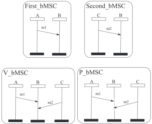
Figure 2.6 presents two bMSCs called respectively F irst_bM SC and Second_bM SC. The sequential composition of these two bMSCs gives the bMSC V _bM SC, and their parallel composition gives the bMSC P _bM SC. The expression F irst_bM SC alt

Second_bM SC means that either F irst_bM SC is executed or Second_bM SC is

executed.

In addition to the seq, alt, par operators, MSC allows the following constructs: • High − level message sequence charts (HM SCs): Here the composition is

described in a automaton like format. they will be described in details in the next section.

• M SC ref erences : MSC references can be used inside an MSC (bMSC or HMSC) to refer to another one. An example of the use of MSC references is presented in Figure 2.7. In this example, the bMSC ref _bM SC contains an MSC reference expression that is attached to the instances A, B, and C and that contains the expression F irst_bM SC alt Second_bM SC. This means that we execute either the bMSC F irst_bM SC or the bMSC Second_bM SC then the instance C sends the message md to D.

(26)

• Inline expressions: These expressions allow the description of the composition of MSCs within an MSC. Figure 2.8 shows an example of the graphical repre-sentation of an inline expression. At the beginning the process K has the choice between sending the message m or the message n.

Figure 2.6: Sequential and parallel composition

(27)

Figure 2.8: Example on MSC Inline Expressions

2.2 High-level Message Sequence Charts

High-level Message Sequence Charts [35] describe the composition of MSCs in a clear and attractive way, which makes it the most used composition mechanism. HMSCs allow to represent the composition situations covered by M SC ref erences and the

Inline expressions as well.

2.2.1 Graphical representation

Graphically an HMSC is represented as a directed graph which nodes are of the form presented in Figure 2.9. A ref erence symbol can contain a reference to a bMSC, another HMSC, or any other M SC ref erence expression. A condition symbol may contain one or several condition names. The start symbol and the end symbol are respectively the initial and the terminal nodes of an HMSC.

Every HMSC should have exactly one start symbol and the graph must be connected so that any node can be reached from the start node. In the directed graph, all nodes have outgoing arrows except an end node, and all have incoming arrows except the

start node.

The connection nodes (called choice nodes) are used mainly when we have several possible choices or alternatives at a point of the HMSC, and they are used as well to connect other nodes to make the HMSC easily readable. A choice node that is directly connected to the start node is called initial node, and the one directly connected to

(28)

Figure 2.9: HMSC symbols types

the end node is called sink node. Figure 2.10 presents a first example of HMSC with two nodes n0, n1, where n0 is the initial node (and also a choice node), and n1 is a

sink node.

Figure 2.10: An example of High-level Message Sequence Chart.

A parallel f rame denotes the parallel composition of one or several HMSCs that it contains. Figure 2.11 shows the graphical representation of a parallel frame.

(29)

Figure 2.11: An example of HMSC with a parallel frame.

2.2.2 Textual representation

As for bMSCs, HMSCs have a textual description. The HMSC from Figure 2.10 is presented textually by:

msc Example ; expr l0 ;

l1: connect seq (l2 alt l3) ; l2: M1 seq (l1) ; l3: M2 seq (l4) ; l4: connect seq (l5) ; l5: end ; endmsc ;

2.2.3 Formal definition

In this thesis we will consider HMSCs without co-regions or parallel frames. This choice is argued in chapter 3 section 3.1.4. The formal definition of the HMSC that we consider can be presented as follows:

Definition 2.2.1 (HMSCs). An HMSC is a graph H = (I, N, →, M, n0, F in), where

(30)

• N is a finite set of nodes, n0 ∈ N is the initial node of H, and Fin ⊆ N is the

set of final states,

• M is a finite set of bMSCs which participating instances belong to I, and defined

on disjoint sets of events,

• →⊆ N × M × N is the transition relation.

In the example of Figure 2.10, M = {M1, M2} and the transition relation contains

two transitions, namely (n0, M1, n0) and (n0, M2, n1). The behavior M1 can be

re-peated an arbitrary number of times, and then be followed by the behavior described in M2. we would like to mention that running M1 followed by M2 does not mean that

all the events described by M1 occur before the ones described by M2 (the process B

might receive the message m2 before receiving m1).

Before giving the definitions of the semantics of HMSC let us formally present Sequen-tial composition of two bMSCs. BMSCs allow for the compact definition of concurrent behaviors but are limited to finite and deterministic interactions. To obtain infinite and non-deterministic specifications, we will use HMSCs, that compose sequentially bMSCs to obtain languages of bMSCs. The sequential composition is formally defined as follows:

Definition 2.2.2 (Sequential composition). Let M1 = (E1, ≤1, C1, φ1, t1, µ1) and

M2 = (E2, ≤2, C2, φ2, t2, µ2) be two bMSCs, defined over disjoint sets of events. The

sequential composition of M1 and M2 is denoted by M1◦ M2. It consists in a

con-catenation of the two bMSCs instance by instance, and is the bMSC M1◦ M2= (E, ≤

, C, φ, t, µ), where:

• E = E1∪ E2, C = C1∪ C2

• ∀e, e′ _{∈ E, e ≤ e}′ _{iff e ≤}

1 e′ or e ≤2 e′ or ∃(e1, e2) ∈ E1 × E2 : φ1(e1) =

φ2(e2) ∧ e ≤1e1∧ e2 ≤2e′

• ∀e ∈ E1, φ(e) = φ1(e), µ(e) = µ1(e), t(e) = t1(e)

• ∀e ∈ E2, φ(e) = φ2(e), µ(e) = µ2(e), t(e) = t2(e)

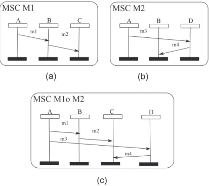
Note that the definition requires the concatenated bMSCs to be defined over disjoint sets of events. In the rest of the chapter, we will use concatenation to assemble several occurrences of the same bMSC. Slightly abusing the definition, we will consider that concatenation M1 ◦ M2 is always defined, and if E1∩ E2 Ó= ∅, we will consider that

(31)

M1◦ M2 is a bMSC obtained by composing M1 with an isomorphic copy of M2 defined

over a set of events that is disjoint from E1. In particular, this allows us to define,

for a bMSC M , the bMSC M ◦ M which denotes a scenario with two consecutive occurrences of M . An intuitive and graphical interpretation for M1◦ M2 is that the

interactions in M2 are appended to M1 after M1 (i.e. drawn below M1). An example

of sequential composition is shown in Figure 2.12: The bMSC M1◦ M2 can simply be

obtained by drawing M2 below M1, and extending the lifelines of instances. Note that

sequential composition does not require both bMSCs to have the same set of instances.

Figure 2.12: Two bMSCs M1 and M2 and their concatenation M1◦ M2

Definition 2.2.3 (HMSC behavior). Let H = (I, N, →, M, n0, F in) be an HMSC.

A path of H is a sequence ρ = (n0, M0, n1)(n1, M1, n2) . . . (nk, Mk, nk+1) of

transi-tions. We will say that a path is acyclic if and only if it does not contain the same transition twice. We define as P aths(H) the set of paths of H starting from the

ini-tial node. A path ρ = (n0, M0, n1) . . . (nk, Mk, nk+1) in P aths(H) defines a sequence

M0.M1. . . Mk ∈ M∗ of bMSCs. We will denote by Mρ the bMSC associated to ρ and

define it as Mρ = M0◦ M1◦ · · · ◦ Mk.

The semantics of an HMSC is given both in terms of generated MSCs FH = { Mρ |

(32)

2.3 MSCs Versions

Message Sequence Charts emerged from the SDL (ITU-T Specification and Descrip-tion Language) community leading to its first ITU-T recommendaDescrip-tion in 1992 . Later there have been revisions of MSC in 1996 [77], in 2000 [35], in 2004 [46], and more recently in 2011 [1]. MSC 2000 differs from MSC-96 mainly in the following areas: better integration of conditions, quantitative notion of time, data specification. We refer the reader to [35] for further details. So far, there exists no formal semantics comparable to the one of MSC-96 for MSC-2000. MSC-2004 is a natural continuation of the MSC-2000 version, refining concepts including: extended data interface, and references to default SDL interface, uni-directional time constraints, and in-line high level expressions. The MSC 2011 is intended to be the same as the 2004 it is only correcting a number of errors into the main text and the appendix. Figure 2.13 shows a brief history of the evolution of the MSC standard.

! ! "

#

$% !

Figure 2.13: Brief history of MSCs.

2.4 Variants of Message Sequence Charts and

similar notations

Several variants of MSCs exist [55]. We present some of the most popular ones in this section.

(33)

2.4.1 Interworkings

Interworkings is a graphical formalism for describing communications between

com-ponents of a system. It also has a formal semantics based on process-algebra [63]. Interworkings were first developed to be used in the analysis phase of the develope-ment process at PKI (Philips Kommunikations Industrie) Nürnberg for the message interactions between blocks [50]. They were also used in the specification of radio communication systems and other industry telecommunication applications. Inter-workings are considered as one of the direct predecessors of MSC-96. However, they can only model synchronous communications which means that messages receptions cannot be delayed as in MSCs, where the communications are asynchronous. Several elements from MSC-96 and other recent versions are absent from Interworkings like asynchronous messages, gates, instance creation and stop, timers, etc. In particu-lar, there is no means for expressing alternatives and repetition, and no referencing mechanism.

2.4.2 UML Sequence Diagram

The UML Sequence Diagrams (SDs for short) are one of the UML diagrams to model the dynamics of a system. Originally, they result from two modeling diagrams: Ivar Jacobson’s interaction diagrams[45], and an Object Oriented variant of MSC-92 lan-guage called OMSC[19]. SDs are very popular for their role within use case driven object oriented software engineering. They are used to describe either the interactions between the system and the actors of its environment or the communications between objects in a system. However, the SDs are not as formal as MSCs. In [78], the authors propose to make a harmonization between the UML SDs and the MSCs so that they have a mutual benefit: MSCs benefit from the popularity of SDs and SDs benefit from all the advantages that offer the MSCs (mainly the composition mechanisms). [34] consider that a specific MSC profile of UML 2.0 could add the innovative data mechanism which possibly could make it easier to handle Interactions formally.

2.4.3 Live Sequence Charts

Live Sequence Charts (LSCs for short)[23] is a language for scenarios, based on

bM-SCs. LSCs provide the means to distinguish mandatory and provisional behaviors during system runs. In [23], the authors relate LSC specifications to system runs. A system run, in their approach, is an infinite sequence of snapshots, where a snapshot

(34)

consists of the set of current events (being either synchronous or asynchronous sends or receives between components or between a component and the environment), and an assignment of values to all variables of the system.

LSCs provide the means to distinguish mandatory and provisional behaviors on the level of the whole chart and three other elements: messages, locations and conditions. This distinction is achieved graphically by using solid line for mandatory LSC element and dashed lines for possible ones. Table 2.14 summarizes the dual mandatory/pro-visional notions supported in LSCs, with their informal meaning: Mandatory charts are classified as Universal LSC and provisional ones as Existential LSC. The distinc-tion regarding an internal chart element is referred to as the element’s temperature; mandatory elements are hot and provisional elements are cold.

! "

# $ Figure 2.14: LSC elements

Furthermore, It is important for a Universal LSC, to state at which point(s) of the run the LSC should be considered, otherwise the behaviors of the entire system have to be specified in one LSC. The authors in [23] define the activation condition and the

pre-chart of an LSC: The activation condition is a boolean condition, which expresses

the activation point of an LSC. The pre-chart allows to specify a prefix or history which must be fulfilled by a run in order to activate the LSC. Pcharts do not re-place the activation condition, but extend it; the activation condition in the presence of a pre-chart indicates the starting point of the prefix. The informal semantics of an LSC with pre-chart is consequently: If the activation condition holds and afterwards

(35)

the pre-chart is completed, then the LSC is activated.

Figure 2.15: Example of LSCs

Figure 2.15 shows an example of two LSCs of a distributed system describing the behaviors of two machines X and Y . The LSC in Figure 2.15-a) is a Universal LSC (solid line) with a pre-chart. When this pre-chart is completed (which means that X sends the message Connect to Y then Y sends the message Connected to X), the chart is activated (X sends the message data to Y then Y sends Ok to X). The LSC in Figure 2.15-b) is an Existential LSC (dashed line) with an activation condition (which is the message badConnection). When the activation condition is satisfied this does not necessarily means that the LSC is activated.

2.4.4 Conclusion

MSC is probably one of the most powerful specification models. The main reason is that it allows to give an hierarchical order to the diagrams and, thereby, describe parallel, sequential and alternative scenarios, and to describe non-regular behaviors as well. All this can be presented in a clear and easy way. However, a disadvantage of MSC, which is also common with other high level specification formalisms, is that the descriptions of these scenarios are not precise enough to derive an equivalent code or an abstract machine model, that we will call in the sequel "implementation".

(36)

2.5 Implementation of Message Sequence Charts

Many researchers consider that, in order to use MSCs in the software life-cycle, it is important that the MSC specification can be translated into distributed state-based specifications (abstract machine models). A natural question is: why not to use di-rectly abstract machine specification? Actually, specifying the system didi-rectly with a state-based specification requires explicit identification of states and thus much more consistency when constructing scenarios. This forces the users to reason about their system in terms of states rather than sequences of actions which is very complex spe-cially for large distributed systems.

Then scenario-based inter-object specifications (e.g., via live sequence charts) and state-based intra-object specifications (e.g., via statecharts) are two complementary ways to specify behavioral requirements. This raises the questions of realizability and implementation. The realizability (or implementability) problem is to know whether we can build an abstract machine model with exactly the same behaviors as the given specification. The implementation problem (or the synthesis) consists in building an abstract machine model with exactly the same behaviors as the given specification. Before formalizing the synthesis problem, we present some of the most important and used abstract machine models.

2.5.1 Abstract machine models

The abstract machine model is the operational model of the system. It describes how each process should behave independently in the system. The code generation is a sim-ple task once an abstract machine model exists. Thus, it is very important to choose a specification model that can be easily translated into an operational model so we can benefit from the specification. As human translation is error-prone, it is important to produce this translation automatically. However, this local view of the specification that each process have in an abstract machine model may add concurrency between the processes. This concurrency might then allow additional behaviors that were not described at the high-level specification. Thus the concurrency is an important point to consider when translating a high-level specification into an abstract machine model. Several abstract machine models appeared in the literature, next we will present only some of the most popular notations.

(37)

2.5.1.1 Petri Nets

Petri nets (PN for short) [68] can be used to describe the state-based behavior of one

instance of the system, or the interactions between several instances as well. It was first introduced in the doctoral thesis of C.A. Petri [73]. Since then the PN model has been developed and applied in a wide range of applications like in communication networks, data flow systems, etc [84]. A Petri Net is a directed bipartite graph with two nodes types: The first, called places, represent conditions. The second, called

transitions, represent the events that may occur. These nodes are connected via

directed arcs such that these arcs never occur between two nodes of the same type. A PN is defined as follows:

Definition 2.5.1 (Petri net). A Petri net is a tuple (P, T, F ), where

• P is a finite set of places, • T is a finite set of transitions, • F ⊆ (P × T) t

(T × P) is a set of arcs (flow relation).

Graphically the places are represented by circles and the transitions by dashes. Several works treated the transformation of MSCs into PN as an abstract machine model [20, 72]. A simple way for representing an MSC by a PN is as follows: The head and the end symbols of instances in a bMSC are represented by a start and an end place for each instance. The MSC events are represented by transitions. A token moving through the net represents the control flows within the system. This token moves from start place to the end place passing all along the transitions and places presenting the occurring MSC events. The Figure 2.16 presents the different representations of MSC events in PN: Figure 2.16(a)for the local actions, Figure 2.16(b) for the sent event and Figure 2.16(c) for receive event. Figure 2.17 presents an example of a transformation of a bMSC into a PN based on the elements presented in Figure 2.16: For each instance in the bMSC we get the events that we transform into Petri net fragments. The resulting Petri net fragments are then composed sequentially in correspondence to the bMSC instances. Finally, the Petri net fragments for the instances are composed in parallel (see [47] for more details). In Figure 2.17, markings of places represent these facts about the system:

– The tokens in places p11, p21 and p31 represent respectively the fact that the processes A, B and C have been started. And the tokens in places p13, p24 and p32 represent respectively the fact that the processes A, B and C have ended.

(38)

Figure 2.16: The representation of some MSC’s events in PN

– p11: represents the fact that the process A has been started, and that A is ready to send the message m1 to the process B.

– p12: A has sent the message m1 to B, and that A is ready to send the message m2 to B.

– p13: A has sent the message m2 to B, and this is the end place for A.

– p21: represents the fact that the process B has been started, and that it is ready to receive the message m1 from the process A.

– p22: B has received the message m1 from A, and that B is ready to send the message m3 to C.

– p23: B has sent the message m3 to C, and that B is ready to receive the message m2 from A.

– p24: B has received the message m2 from A, and this is the end place for B. – p31: represents the fact that the process C has been started, and that it is ready

to receive the message m3 from the process B.

– p24: C has received the message m3 from B, and this is the end place for C. – A token in the place p121 represents the message m1.

– A token in the place p122 represents the message m2. – A token in the place p321 represents the message m3. The transitions represent the following activities in the system:

– t11: A sends the message m1 to B, – t21: B receives the message m1 from A, – t12: A sends the message m2 to B, – t23: B receives the message m2 from A, – t22: B sends the message m3 to C,

(39)

– t31: C receives the message m3 from B,

Figure 2.17: The transformation of a bMSC into a PN

The implementation of an HMSC with Petri nets results in additional behaviors [20]. for instance let us consider the example of HMSC of Figure 2.18.

If the process A of the HMSC of Figure 2.18 sends the message m1 then the message

m2 to the process B, then B must receive the message m1 before receiving the message m2 what might not be the case in the corresponding Petri Net presented in Figure 2.19

Then, one shall notice that HMSCs semantics can enforce messages between a pair of processes to respect FIFO ordering (that we will explain in chapter 3), which cannot be enforced by Petri nets. In fact, it has been shown that synthesis of Petri nets from HMSCs usually produces an overapproximation of the initial HMSC language [20]. So PN cannot be used as implementation model.

2.5.1.2 Statecharts

Statecharts are synchronous languages originally introduced by Harel in [33]. They

are a variant of the Finite State Machines (denoted FSMs). FSM is a model of com-putation that consists of a set of states, a start state, an input alphabet, a transition functions, and accepting states. The computation begins at the start state, then it

(40)

Figure 2.18: Example of HMSC

(41)

changes to a new state for each event/message (an event is somethig that occurs in the system like an input from the environment, a message, etc.) depending on the tran-sition function. Statecharts have extended the FSMs with some additional features like hierarchy and parallelism, and broadcast communications. Statecharts formalism continue evolving over the years, spawning many variants like classical statecharts (or Harel’s Statecharts) UML Statecharts, and Rhapsody Statecharts [22].

It is clearly stated in the Z.120 standard [35] that bMSCs and HMSCs depict the behavior of agents that communicate asynchronously, which rules out statecharts as a possible abstract machine model. In [49] the authors consider the transformation of a finite set of bMSCs into statecharts but the communications are supposed syn-chronous. Some other works deal with the transformation of HMSCs into statecharts but they change HMSCs semantics so that the execution of a bMSC does not start while the execution of the previous bMSC have not yet ended. In the method of syn-thesis that we propose in chapter 3, we will not change the semantics of the HMSC [58], and yet implement correctly a subset of the language.

2.5.1.3 Communicating Finite State Machine

Communicating F inite State M achines (CFSM for short) [17] appeared as one of

the earliest abstract machine models to represent distributed systems [18, 87], and are used for instance in the specification language SDL. A CFSM A is a network of finite state machines that communicate over unbounded, non-lossy, error-free and FIFO communication channels. One state machine is presented as a directed labeled graph where nodes represent states and edges represent transitions. A transition between two states can be either a send or a receive or a local transition. An edge is labeled by

p!q(m) (when the current machine named p sends a message m to another machine

named q), or by p?q(m) (when the current machine named p receives a message m from another machine named q), or by a (where a is the name of a local action of the current machine). Each state in a state machine has at least one output edge except the final state. One of the states is identified as its initial state; and all states are reachable from the initial state. A subset of states, called accepting states (or final states), are states that mark a successful run which is a run that ends with emtpy buffers. We give a formal definition of CFSM and their semantics in chapter 3 section 3.

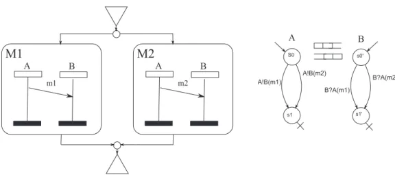
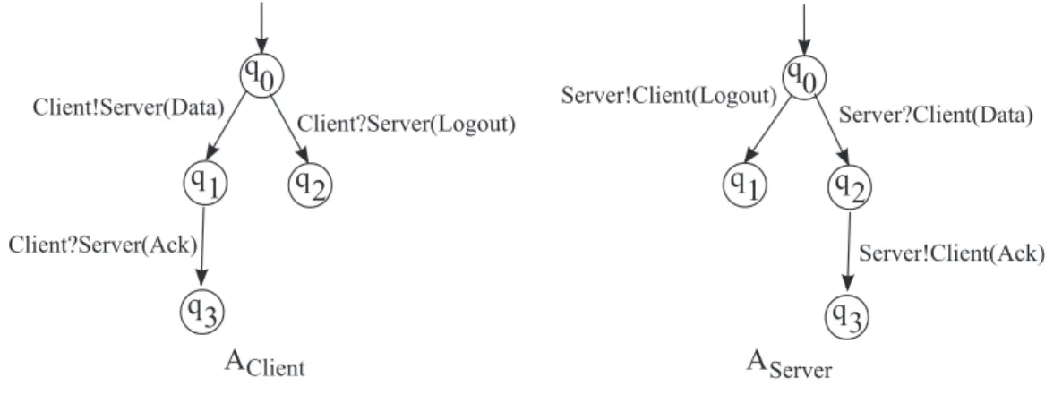
Figure 2.20 presents an HMSC and two CFSMs A and B that describe the behaviors of the two processes in the HMSC. The initial states of these two machines are

(42)

de-Figure 2.20: Two communicating machines.

noted by a dark incoming arrow and the final states by a cross.

The tight relationship of CFSMs with MSCs is well known [56, 8]. For instance, Lohrey in [56] considers that an accepting run of a CFSM generates in a canonical way an MSC. In the sequel, we choose CFSM model as the implementation model, so we will mainly focus on realizability and implementation problems for HMSCs and CFSMs.

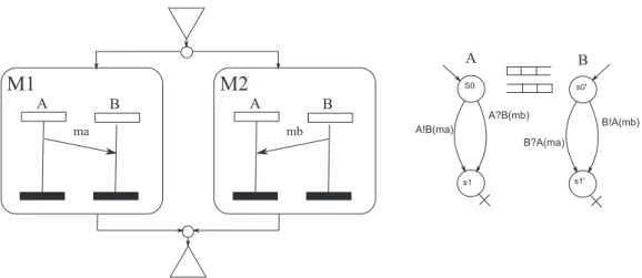
Actually the synthesis of an HMSC into a CFSM might contain deadlocks. For in-stance let us consider the figure 2.21 that presents an HMSC and its corresponding CFSM. In this example, if the process A sends the message ma to the process B and at the same time the process B sends the message mb to the process A; In this case the two corresponding communicating automata will be respectively at the states s1 and

s1′ _{with the two messages ma and mb in their respective buffers. This is a deadlock}

situation.

The semantics of CFSMs is usually defined as the set of runs that do not lead to deadlocks. The events that occur and lead a run to deadlock should not appear in the semantics, thus these events are canceled. We consider that allowing deadlocks in an implementation, and considering that we can simply cancel the events that lead to deadlock is not a realistic solution. In the real life applications (like avionics), events cannot be canceled simply by undoing them. In the synthesis algorithm that we will propose in chapter 3, we consider as semantics of CFSM all prefixes of extensions of the network of machines, including prefixes of executions that end on a deadloack.

(43)

Figure 2.21: Example of a CFSM that might deadlock.

(44)

2.5.2 The realizability and the synthesis of HMSCs

The synthesis of a scenario-based model consists in building an abstract machine model with exactly the same behaviors as the scenario-based model. Several patholo-gies in scenario-based models that prevent their synthesis have been studied. An overview of 21 approaches is given in [55] where the authors compare some of the al-gorithms that generate abstract machine models from scenario-based models that have been proposed in the literature. The differences and similarities of the approaches are identified using two sets of comparison criteria: criteria relevant from a user’s perspec-tive (Intended use, Support of parallelism, Support of composition mechanism, etc), and criteria relevant from a technical perspective (Consistency check: The require-ments can be semantically inconsistent, Completeness check: the behaviors inferred from the synthesized abstract machine models may not be equal to the behaviors specified by the specification models, etc.). One of their goals is to identify the dif-ferences and similarities among approaches and highlight them in the comparison results. The other goal is to explore some of the challenges that current approaches may face are: the implied scenarios (the additional behaviors that were not described in the specification), the consistency (e.g., the synthesized model contains deadlocks), the support of parallelism or concurrency (They noticed that more than half of the approaches do not support parallelism. The reason behind this may be related to the computational complexity typically introduced by the support of parallelism that we explain in chapter 3 section 3.1.4 ), etc.

Next we will consider works about the synthesis of MSCs specifications. Some of these works consider the synthesis of bMSCs into abstract machine models. A bMSC depicts the exchange of messages among the communicating entities in a distributed system, it contains neither loops nor alternatives and then it corresponds to a single execution of the system that describe a finite set of behaviors. Therefore, a finite set of bMSCs also describes a finite set of behaviors. In [7], the authors study the synthesis of CFSM from a set of bMSCs, and present an algorithm that detects other unspecified and possibly unwanted scenarios called implied scenarios. Thereby, if we have no implied scenarios then there is an algorithm that can synthesize CFSM with exactly the same behaviors as the specification. The authors present two notions of realizability, depending on whether the realization is required to be deadlock-free (safe realizability) or not (weak realizability).

(45)

richer formalisms and HMSCs have received a quite attention for this. Several works consider synthesis of HMSC specifications into abstract machine models. For instance, [48] considers a synthesis method that translates an HMSC into SDL specifications, by projection (that is build one communicating agent per process) of the HMSC on its instances. However, the generated SDL system allows more traces than those defined by the HMSC specification. This is due to the impossibility of preserving an order between message receptions from different senders. The projection on processes does not preserve this order. It is the same for [20] that considers the implementation of HMSCs by Petri nets but with a larger set of behaviors. In the sequel, and as we have chosen CFSM as the implementation model, we will mainly focus on realizability and implementation problems for HMSCs and CFSMs.

The realizability (or implementability) problem of HMSCs into CFSMs consists in deciding whether we can build a CFSM with exactly the same behaviors as the given HMSC. Some works [8, 83] present two notions of realizability depending on whether we require the implementation to be deadlock-free (safe realizability) or not (weak realizability). The question about the realizability of the HMSCs by CFSMs was studied in several approaches [7, 8, 31]. These studies show that this realizability is in general undecidable, unless the specifications meet some restrictions. In [56], Lohrey prove that the realizability of HMSCs into CFSMs is undecidable for class of general HMSCs. Thus several sub-classes of HMSCs that have synthesis algorithms were presented in the literature. Trivially the realizability of these sub-classes into CFSMs is decidable.

2.5.2.1 Globally-cooperative HMSC

The Globally-cooperative HMSCs have been introduced in [66]. Before introducing the definition of Globally-cooperative HMSCs let us define the communication Graph of a bMSC:

Definition 2.5.2 (communication Graph of a bMSC). The communication graph of

a bMSC M is the directed graph G(I,Ô→) where I is the set of active instances of M : , and such that for i ∈ I and j ∈ I, (i, j) ∈ Ô→, if there exists an event e=i!j(m). An MSC is called connected (resp. strongly connected) if its communication graph is connected (resp. strongly connected). Communication graphs are useful to classify high-level MSCs.

(46)

Definition 2.5.3 (Globally-cooperative HMSC). An HMSC H = (I, N, →, M, n0)

is called globally-cooperative, if for every cycle ρ in H, Mρ has a weakly connected

communication graph.

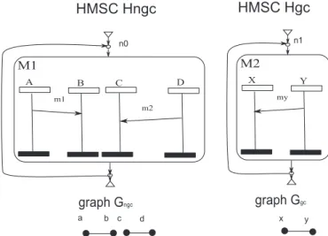
In Figure 2.23, the HMSC Hngc is not a globally-cooperative HMSC, since Gngc, the

communication graph corresponding to (n0,M1,n0) in Hngc, has two weakly connected

components one over A,B and the other over C,D. The HMSC Hgc is a

globally-cooperative HMSC as Ggc, the communication graph corresponding to (n1,M2,n1) in

Hgc, is a weakly connected graph.

Figure 2.23: globally-cooperative HMSCs

Globally-cooperative HMSCs are always implementable by a CFSM but with possi-ble deadlocks [30]. There is an EXPSPACE-complete algorithm to test whether a globally-cooperative HMSC is implementable with a deadlock-free CFSM and with-out additional data [56]. However, it is clear that the algorithm is obviously time-consuming, and sometimes even some easily implementable HMSC are considered not deadlock-free implementable, as the globally-cooperative HMSC of Figure 2.24 [29]. At node n0 we have a similar situation as for the example of the Figure 2.21 that lead to a deadlock. Such situation will be called a non-local choice, and will be discussed in details in chapter 3.

(47)

Figure 2.24: HMSC depicting the transactions of usb 1.1

2.5.2.2 Regular HMSC

Another subclass of HMSC, the regular HMSCs, was introduced in [10].

Definition 2.5.4 (Regular HMSC). An HMSC H is called regular, if every bMSC

labeling a loop of H has a strongly connected communication graph.

The HMSC Hreg presented in the figure 2.25 is a regular HMSC. A regular HMSC

is a globally-cooperative HMSC with bounded communication channels (buffers have bounded contents in any execution).

Figure 2.25: Regular HMSC

The authors in [67] proved that any regular set of MSCs admits a deterministic imple-mentation with bounded channel capacities up to some additional message contents

(48)

called time-stamps. This result shows the power of adding contents to messages com-pared to the more restrictive approach proposed in [7] where no additional message content is allowed. For non-FIFO communications systems [66] proved that weak realizability is decidable for bounded HMSCs. The work in [7] was extended in [8] to consider realizability of bounded HMSCs. In [8], the authors proved that for FIFO communication systems weak realizability is, surprisingly, undecidable for bounded MSC-graphs, while safe realizability is in Expspace. However, the question of the exact complexity remains open. In [56], Lohrey prove that for FIFO communications safe realizability is EXPSPACE-complete for bounded HMSCs and that under non-FIFO communication weak realizability is EXPSPACE-hard for bounded HMSCs. [13] extends [67] and consider non-FIFO communication, and identify a subclass of HMSCs (called coherent HMSCs), which are safely realizable with additional message contents. However, checking whether an HMSC is coherent is in general difficult. Co-herence is undecidable for HMSCs, and EXPSPACE-complete for locally synchronized HMSCs and for globally cooperative HMSCs. (theorem 5.1 in [13]).

2.5.2.3 Locally-cooperative HMSC

The locally-cooperative HMSCs sub-class was introduced in [31] and is a sub-class of globally-cooperative HMSCs.

Definition 2.5.5 (locally-cooperative HMSC). An HMSC H = (I, N, →, M, n0) is

called locally − cooperative, if for every bMSCs M 1 and M 2 such that (n0,M 1,n1) ∈

→ and (n1,M 1,n2) ∈ →, the bMSCs M 1,M 2 and M 1 ◦ M 2 all have weakly connected

communication graphs.

Implementability of distributed systems described with scenarios

HAL Id: tel-00919684

https://tel.archives-ouvertes.fr/tel-00919684

Implementability of distributed systems described with

scenarios

Rouwaida Abdallah

To cite this version:

Implementability of distributed systems described

with scenarios

Abstract

Table of Contents

Thank you

Chapter 1

Introduction

1.1

Context

1.2

Motivation

1.3

The synthesis problem

1.4

Contribution

1.4.1

Any local HMSC is correctly implementable

1.4.2

The synthesis of non-local HMSCs

1.4.3

SOFAT tool

1.5

Thesis organization

Chapter 2

State of the art

2.1

Basic Message Sequence Charts

2.1.1

Graphical representation

2.1.2

Textual representation

2.1.3

Formal definition

2.1.4

Events Ordering and Co-regions

2.1.5

Gates

2.1.6

MSC composition

2.2

High-level Message Sequence Charts

2.2.1

Graphical representation

2.2.2

Textual representation

2.2.3

Formal definition

2.3

MSCs Versions

2.4

Variants of Message Sequence Charts and

similar notations

2.4.1

Interworkings

2.4.2

UML Sequence Diagram

2.4.3

Live Sequence Charts

2.4.4

Conclusion

2.5

Implementation of Message Sequence Charts

2.5.1

Abstract machine models

2.5.2

The realizability and the synthesis of HMSCs