HAL Id: hal-01985695
https://hal.archives-ouvertes.fr/hal-01985695
Preprint submitted on 18 Jan 2019HAL is a multi-disciplinary open access archive for the deposit and dissemination of sci-entific research documents, whether they are pub-lished or not. The documents may come from teaching and research institutions in France or abroad, or from public or private research centers.
L’archive ouverte pluridisciplinaire HAL, est destinée au dépôt et à la diffusion de documents scientifiques de niveau recherche, publiés ou non, émanant des établissements d’enseignement et de recherche français ou étrangers, des laboratoires publics ou privés.
Decay of semilinear damped wave equations: cases
without geometric control condition
Romain Joly, Camille Laurent
To cite this version:
Romain Joly, Camille Laurent. Decay of semilinear damped wave equations: cases without geometric control condition. 2019. �hal-01985695�
Decay of semilinear damped wave equations:
cases without geometric control condition
Romain Joly∗ & Camille Laurent†‡
Abstract
We consider the semilinear damped wave equation
∂tt2u(x, t) + γ(x)∂tu(x, t) = ∆u(x, t)− αu(x, t) − f(x, u(x, t)) .
In this article, we obtain the first results concerning the stabilization of this semilin-ear equation in cases where γ does not satisfy the geometric control condition. When some of the geodesic rays are trapped, the stabilization of the linear semigroup is semi-uniform in the sense that ∥eAtA−1∥ ≤ h(t) for some function h with h(t) → 0
when t → +∞. We provide general tools to deal with the semilinear stabilization problem in the case where h(t) has a sufficiently fast decay.
Keywords: damped wave equations; stabilization; semi-uniform decay; unique
con-tinuation property; small trapped sets; weak attractors.
Contents
1 Introduction 2
2 Notations and basic facts 8
3 Asymptotic compactness and reduction to a unique continuation problem 9 4 Rate of the nonlinear decay: proof of Proposition 1.3 12
4.1 The polynomial case . . . 12 4.2 The exponential case . . . 14
5 Application 1: the open book 15
6 Unique continuation theorems 16
6.1 Unique continuation with coefficients analytic in time . . . 16 6.2 Unique continuation through pseudo-convex surfaces without boundary . . 16 6.3 Unique continuation through pseudo-convex surfaces with boundary . . . . 20 6.4 Proof of Theorem 1.2 . . . 21
7 Application 2: the peanut of rotation 21
∗Universit´e Grenoble Alpes, CNRS, Institut Fourier, F-38000 Grenoble, France, email:
romain.joly@univ-grenoble-alpes.fr
†CNRS, UMR 7598, Laboratoire Jacques-Louis Lions, F-75005, Paris, France
‡UPMC Univ Paris 06, UMR 7598, Laboratoire Jacques-Louis Lions, F-75005, Paris, France, email:
8 Decay estimate in the disk with holes 23
9 Application 3: the disk with two holes 26
10 Analytic regularization and proof of Theorem 1.1 27 10.1 Analytic regularization of global bounded solutions . . . 27 10.2 Proof of Theorem 1.1 . . . 32
11 Application 4: the disk with many holes 33
12 Application 5: Hyperbolic surfaces 34
13 A uniform bound for the H2× H1-norm 34
A Estimates of the resolvent and decay of the semigroup 36 B Estimates of the resolvent of abstract damped wave equations 38 C Estimates for the high-frequencies projections 40
1
Introduction
We consider the semilinear damped wave equation
∂tt2u(x, t) + γ(x)∂tu(x, t) = ∆u(x, t)− αu(x, t) − f(x, u(x, t)) (x, t)∈ Ω × (0, +∞)
u|∂Ω(x, t) = 0 (x, t)∈ ∂Ω × (0, +∞)
(u(·, t = 0), ∂tu(·, t = 0)) = U0 = (u0, u1)∈ H01(Ω)× L2(Ω)
(1.1) in the following general framework:
(i) the domain Ω is a two-dimensional smooth compact and connected manifold with or without smooth boundary. If Ω is not flat, ∆ has to be taken as Beltrami Laplacian operator.
(ii) the constant α ≥ 0 is a non-negative constant. We require that α > 0 in the case without boundary to ensure that ∆− αId is a negative definite self-adjoint operator. (iii) the damping γ∈ L∞(Ω,R+) is a bounded function with non-negative values. Since we want to consider a damped equation, we will assume that γ does not vanish everywhere.
(iv) the non-linearity f ∈ C1(Ω×R, R) is of polynomial type in the sense that there exists a constant C and a power p≥ 1 such that for all (x, u) ∈ Ω × R,
|f(x, u)| + |∇xf (x, u)| ≤ C(1 + |u|)p and |fu′(x, u)| ≤ C(1 + |u|)p−1 . (1.2)
Moreover, in most of this paper, we will be interested in the stabilization problem and we will also assume that
We introduce the space X = H01(Ω)× L2(Ω) and the operator A defined by D(A) = (H2(Ω)∩ H01(Ω))× H01(Ω) A = ( 0 Id ∆− αId −γ(x) ) .
In this paper, we are interested in the cases where the linear semigroup eAthas no uniform decay, that is that ∥eAt∥L(X) does no converge to zero. We only assume a semi-uniform decay, but sufficiently fast in the following sense.
(v) There exist a function h(t) such that
∀U0 ∈ D(A) , ∥eAtU0∥X ≤ h(t) ∥U0∥D(A) (1.4)
and there is σh∈ (0, 1] such that
lim
t→∞h(t) = 0 and ∀σ ∈ [0, σh] ,
∫ ∞ 0
h(t)1−σdt < ∞ . (1.5)
Condition (1.5) requires a decay rate fast enough to be integrable. Roughly speaking, this article shows that this condition, together with a suitable unique continuation property, are sufficient to obtain a stabilization of the semilinear equation. The relevant unique continuation property is explained in Proposition 3.5 below. We present two general results where it can be obtained.
Our first result concerns analytic nonlinearities and smooth dampings.
Theorem 1.1. Consider the damped wave equation (1.1) in the framework of Assumptions (i)-(v). Assume in addition that:
a) the function (x, u)7→ f(x, u) is smooth and analytic with respect to u.
b) the damping γ is of class C1 or at least that there exists ˜γ ∈ C1(Ω,R+) such that (v)
holds with γ replaced by ˜γ and such that the support of ˜γ is contained in the support of γ.
c) the power p of f in (1.2) and the decay rate h(t) of the semigroup in (1.4) satisfy h(t) =O(t−β) with β > 2p.
Then, any solution u of (1.1) satisfies ∥(u, ∂tu)(t)∥H1
0×L2 −−−−−−−−→t−→+∞ 0 .
Moreover, for any R and σ > 0, there exists hR,σ(t) which goes to zero when t goes to
+∞ such that the following stabilization hold. For any U0 ∈ H01+σ(Ω)× Hσ(Ω), if u is
the solution of (1.1), then
∥(u0, u1)∥H1+σ×Hσ ≤ R =⇒ ∥(u, ∂tu)(t)∥H1
0×L2 ≤ hR,σ(t) −−−−−−−−→t−→+∞ 0 .
Our assumptions (v) and c) on the decay of the linear semigroup may seem strong. They are satisfied in the cases where the set of trapped geodesics, the ones which do not meet the support of the damping, is small and hyperbolic in some sense. Several geometries satisfying (v) and c) have been studied in the literature, see the concrete examples of Figure 1 and the references therein. Notice in particular that the example of domain with holes is particularly relevant for applications where we want to stabilize a nonlinear material with
holes by adding a damping or a control in the external part. There is a huge literature about the damped wave equation and the purpose of the examples presented here is mainly to illustrate our theorem to non specialists. Moreover, the subject is growing fastly, giving more and more examples of geometries where we understand the effect of the damping and where we may be able to apply our results. We do not pretend to exhaustivity and refer to the bibliography of the more recent [25] for instance.
In some cases, the unique continuation property required in Proposition 3.5 can be obtained without considering analytic nonlinearities or conditions on the growth of f as Hypothesis c) of Theorem 1.1. Instead, we require a particular geometry, which will be introduced more precisely in Section 6.
Theorem 1.2. Consider the damped wave equation (1.1) in the framework of Assumptions (i)-(v). Assume in addition that:
a) the function (x, u)7→ f(x, u) is of class C1(Ω× R, R).
b) there exists a pseudo-convex foliation of Ω in the sense of Definitions 6.4 or 6.6. Then, the conclusions of Theorem 1.1 hold.
This result can be applied in several situations of Figure 1: the “disk with two holes”, the “peanut of rotation” and the “open book”. In these cases, the stabilization holds for any natural nonlinearity.
We expect that the decay rate hR,σ(t) is related to the linear decay rate h(t) of
As-sumption (v). We are able to obtain this link for the typical decays of the examples of Figure 1.
Proposition 1.3. Consider a situation where the stabilization stated in Theorems 1.1 or
1.2 holds. Then,
• if the decay rate of Assumption (v) satisfies h(t) = O(t−α) with α > 1, then the
nonlinear equation admits a decay of the type hR,σ(t) =O(t−σα).
• if the decay rate of Assumption (v) satisfies h(t) = O(e−at1/β
) with a > 0 and β > 0,
then the nonlinear equation admits a decay of the type hR,σ(t) =O(e−bσt
1/(β+1)
) for
some b > 0.
Notice that this result is purely local in the sense that the decay rate is obtained when the solution is close enough to 0. Our proofs do not provide an explicit estimate of the time needed to enter this small neighborhood of 0. Also notice that the loss in the power of the second case of Proposition 1.3 is due to an abstract setting: in the concrete examples, we may avoid this loss, see the remark below Lemma 4.2 and the concrete applications to the examples of Figure 1.
To our knowledge, Theorems 1.1 and 1.2 are the first stabilization results for the semi-linear damped wave equation when the geometric control condition fails. This famous geometric control condition has been introduced in the works of Bardos, Lebeau, Rauch and Taylor (see [4]) and roughly requires that any geodesic of the manifold Ω meets the support of the damping γ. This condition implies that the linear semigroup of the damped wave equation satisfies a uniform decay∥eAt∥L(H1
0×L2)≤ Me
−λt. In this context, the
sta-bilization of the semilinear damped wave equation has been studied since a long time, see for example [19, 44, 14, 15, 27]. Under this condition and for large data, the proof often divides into a part dealing with high frequencies with linear arguments and another
'
&
$
%
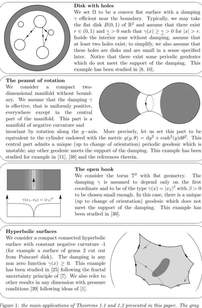
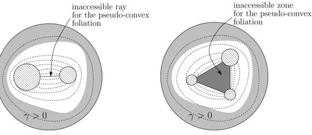
Disk with holes
We set Ω to be a convex flat surface with a damping
γ efficient near the boundary. Typically, we may take
the flat disk B(0, 1) of R2 and assume that there exist
r ∈ (0, 1) and γ > 0 such that γ(x) ≥ γ > 0 for |x| > r.
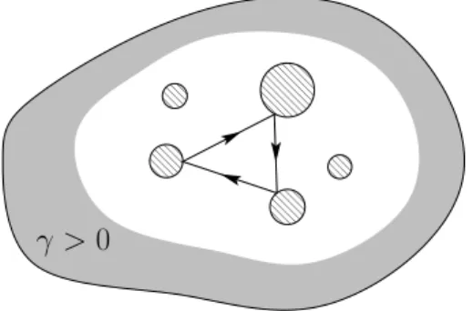
Inside the interior zone without damping, assume that at least two holes exist; to simplify, we also assume that these holes are disks and are small in a sense specified later. Notice that there exist some periodic geodesics which do not meet the support of the damping. This example has been studied in [8, 10].
'
&
$
%
The peanut of rotation
We consider a compact two-dimensional manifold without bound-ary. We assume that the damping γ is effective, that is uniformly positive, everywhere except in the central part of the manifold. This part is a manifold of negative curvature and
invariant by rotation along the y−axis. More precisely, let us set this part to be equivalent to the cylinder endowed with the metric g(y, θ) = dy2 + cosh2(y)dθ2. This central part admits a unique (up to change of orientation) periodic geodesic which is unstable; any other geodesic meets the support of the damping. This example has been studied for example in [11], [38] and the references therein.
'
&
$
%
γ(x1, x2) =|x1|β
The open book
We consider the torus T2 with flat geometry. The damping γ is assumed to depend only on the first coordinate and to be of the type γ(x) = |x1|β with β > 0 to be chosen small enough. In this case, there is a unique (up to change of orientation) geodesic which does not meet the support of the damping. This example has been studied in [30]. ' & $ % Hyperbolic surfaces
We consider a compact connected hyperbolic surface with constant negative curvature -1 (for example a surface of genus 2 cut out from Poincar´e disk). The damping is any non zero function γ(x) ≥ 0. This example has been studied in [25] following the fractal uncertainty principle of [7]. We also refer to other results in any dimension with pressure conditions [39] following ideas of [1].
Figure 1: the main applications of Theorems 1.1 and 1.2 presented in this paper. The gray
parts show the localization of the damping (white=no damping). The more geometrically constrained Theorem 1.2 apply to the “disk with two holes”, the “peanut of rotation” and the “open book”.
one dealing with low frequencies that often requires a unique continuation argument. The high frequency problem was solved by Dehman [14] with important extension by Dehman-Lebeau-Zuazua [15] using microlocal defect measure. Yet, the unique continuation was proved by classical Carleman estimates (see Section 6.2 below) which restricted the gen-erality of the geometry. Using techniques from dynamical systems applied to PDEs, the authors of the present article proved in [27] a general stabilization result under Geometric Control Condition, at the cost of an assumptions of analyticity of the nonlinearity. The-orem 1.1 is in the same spirit as [27] and intends to prove that related techniques can be extended to a weaker damping. Theorem 1.2 is more in the spirit of the other references, taking advantage of particular geometries, but avoiding analyticity.
Notice that the “disk with one hole” satisfies this geometric control condition and thus it is not considered in this paper.
In the cases where the geometric control condition fails, the decay of the linear semi-group is not uniform. At least, if γ does not vanish everywhere, it is proved in [12] (see also [19]) that the trajectories of the linear semigroup goes to zero (see Theorem 2.1 below). In fact, the decay can be estimated with a loss of derivative as
∥eAtU∥
H1×L2 ≤ h(t)∥U∥H2×H1 with h(t)−−−−−→
t→+∞ 0 . (1.6)
In the general case, as soon as γ̸≡ 0, the decay rate can be taken as h(t) = O(ln(ln(t))/ ln t) as shown in [31, 32]. In some particular situations, γ misses the geometric control condition but very closely: typically there is only one (up to symmetries) geodesic which does not meet the support of the damping and this geodesic is unstable. In this case, we may hope a better decay than theO(ln(ln(t))/ ln t) one, see for example [11, 30] and the other references of Figure 1.
To our knowledge, until now, there was no result concerning the semilinear damped wave equation (1.1) when the geometric control condition fails. Thus Theorems 1.1 and 1.2 provides the first examples of semi-uniform stabilization for the semilinear damped wave equation. Notice that our results deeply rely on the fact that the decay rate of (1.6) is integrable. Typically, for the situations of Figure 1, it is of the type h(t) =O(e−λtα) or
h(t) =O(1/tβ) with sufficiently large β > 0.
Theorems 1.1 and 1.2 concern the stabilization of the solutions of (1.1) in the sense that their H1× L2-norm goes to zero. Notice that, since the energy of the damped wave equation is non-increasing (see Section 2), we knew that this H1× L2-norm is at least bounded. Such a uniform bound is not clear a priori for the H2× H1-norm. However, basic arguments provide this bound as a corollary of Theorems 1.1 and 1.2 if the decay is fast enough, which is the case of the “disk with holes”, the “peanut of rotation” and the “hyperbolic surfaces” of Figure 1.
Theorem 1.4. Consider the damped wave equation (1.1) in the framework of Theorems
1.1 or 1.2. Assume that for all R > 0, the decay rate hR,1(t) is faster than polynomial,
i.e. hR,1(t) = o(t−k) for any k ∈ N. Also assume that γ is of class C1 and f is of class
C2(Ω×R, R). Then the H2(Ω)×H1(Ω)-norm of the solutions are bounded in the following
sense. For any R > 0, there exists C(R) > 0 such that, for any U0∈ (H2(Ω)∩ H01(Ω))×
H01(Ω) such that ∥U0∥H2×H1 ≤ R, the solution u of (1.1) satisfies
sup
t≥0∥(u, ∂
tu)(t)∥H2×H1 ≤ C(R) .
Note that, in the case without damping, this result is sometimes expected to be false. It is related to the weak turbulence, described as a transport from low frequencies to high frequencies.
The main purpose of this paper is to obtain new examples of stabilization for the semilinear damped wave equation and to introduce the corresponding methods and tools. We do not pretend to be exhaustive and the method may be easily used to obtain further or more precise results. For example:
• the boundary condition may be modified, typically in the case of the disk with holes,
Neumann boundary condition may be chosen at the exterior boundary.
• for simplicity, the examples of Figure 1 and the main results of this article concern
two-dimensional manifolds. However, the arguments of this paper can be used to deal with higher-dimensional manifolds. There are some technical complications, mainly due to the Sobolev embeddings. For example, in dimension d = 3, the degree of f in (1.2) should satisfy p < 3 (p < 5 if we use Strichartz estimates as done in [27] using [15]) and the order β of the vanishing of γ in the example of the open book should not be too large. To simplify, we choose to state our results in dimension
d = 2. However, several intermediate results in this article are stated for dimensions d = 2 or d = 3.
• It is also possible to combine the strategy of this paper with other tricks and technical
arguments. For example, we may consider unbounded manifolds or manifolds of dimension d = 3 with nonlinearity of degree p ∈ [3, 5), which are supercritical in the Sobolev sense. This would requires to use Strichartz estimates in addition to Sobolev embeddings as done in [15] or [27].
• assume that we replace the sign condition (1.3) by an asymptotic sign condition ∃R > 0 , ∀(x, u) ∈ Ω × R , |u| ≥ R ⇒ f(x, u)u ≥ 0 .
Then they may exist several equilibrium points and the stabilization to zero cannot be expected. However, the arguments of this paper show that the energy E intro-duced in Section 2 is a strict Lyapounov functional and that any solution converges to the set of equilibrium points. We can also show the existence of a weak compact
at-tractor in the sense that there is an invariant compact setA ⊂ H01(Ω)×L2(Ω), which consists of all the bounded trajectories and such that any regular set B bounded in (H2(Ω)∩H01(Ω))×H01(Ω) is attracted byA in the topology of H01(Ω)×L2(Ω). Notice that this concept of weak attractor is the one of Babin and Vishik in [3]. At this time, the asymptotic compactness property of the semilinear damped wave equation was not discovered and people thought that a strong attractor (attracting bounded sets of H01(Ω)× L2(Ω)) was impossible due to the lack of regularization property for the damped wave equation. Few years later, Hale [17] and Haraux [19] obtain this asymptotic compactness property and the existence of a strong attractor. Thus this notion of weak attractor has been forgotten. It is noteworthy that it appears again here. Notice that we cannot hope a better attraction property since even in the linear case, {0} is not an attractor in the strong sense.
The organization of this paper follows the proof of stabilization of the examples of Figure 1. We add step by step the techniques required to deal with our guiding examples, from the simplest to the most complicated one.
Sections 2 and 3 contain the basic notations and properties. The asymptotic com-pactness of the semilinear dynamics is proved and the problem is reduced to a unique continuation property. In Section 4, we show the estimations of Proposition 1.3. Sec-tion 5 then proves the nonlinear stabilizaSec-tion in the “open book” case, where the unique
continuation property is trivial. Section 6 stated several unique continuation results, en-abling to prove Theorem 1.2. We obtain as a consequence the stabilization in the case of the “peanut of rotation” in Section 7. Section 8 studies the linear semigroup for the case of the “disk with holes” before we apply Theorem 1.2 in the case of the “disk with two holes” in Section 9. Theorem 1.1 is proved in Section 10 by showing an asymptotic analytic regularization. It is applied to the “disk with three or more holes” and hyperbolic surfaces, assuming f analytic in u, in Sections 11 and 12. In Section 13, we show how to obtain Theorem 1.4 as a corollary of Theorems 1.1 or 1.2. This article finishes with three appendices on the links between the decay of the semigroup eAt and the resolvent (A− iµId)−1.
Acknowledgements: The authors deeply thank Matthieu L´eautaud for his contributions to the appendices. They are also grateful to Nicolas Burq for several discussions and the suggestion of Theorem 1.4. Part of this work has been made in the fruitful atmosphere of the Science Center of Benasque Pedro Pascual and has been supported by the project
ISDEEC ANR-16-CE40-0013.
2
Notations and basic facts
We use the notations of Equation (1.1), of Assumptions (i)-(v) and of the introduction. In particular, we recall that X = H01(Ω)× L2(Ω) and
D(A) = (H2(Ω)∩ H01(Ω))× H01(Ω) A = ( 0 Id ∆− αId −γ(x) ) .
The operator A is the classical linear damped wave operator corresponding to the linear part of (1.1). Due to Lumer-Phillips theorem, we know that this operator generates a linear semigroup of contractions eAt on X and on D(A) and that
∀t ≥ 0 , ∥eAt∥
L(X) ≤ 1 and ∥eAt∥L(D(A))≤ 1 .
Notice that the second estimate is a direct consequence of the commutation of A and eAt and does not require any regularity on γ.
For any σ∈ [0, 1], we set
Xσ = (H1+σ(Ω)∩ H01(Ω))× H0σ(Ω) .
Thus X0 = X and X1= D(A) and Xσ is an interpolation space between X0 and X1. In particular, by interpolation, eAt is defined in Xσ and we have
∀σ ∈ [0, 1] , ∀t ≥ 0 , ∥eAt∥
L(Xσ) ≤ 1 . (2.1) We set F ∈ C0(X) to be the function
F : U = ( u v ) ∈ X 7−→ ( 0 −f(·, u) ) ∈ X . (2.2)
Notice that, if Ω is two-dimensional, H01(Ω) ,→ Lp(Ω) for any p∈ [1, +∞) and if Ω is three-dimensional H01(Ω) ,→ L6(Ω). Thus, f (u) is well defined in L2(Ω) due to Assumption (1.2)
if dim(Ω) = 2 or if dim(Ω) = 3 and p≤ 3. Moreover, for any R, u and v with ∥u∥H1 ≤ R and∥v∥H1 ≤ R, we have ∥f(·, u) − f(·, v)∥L2 = (u − v)∫01fu′(·, u + s(u − v))ds L2 ≤ C(R)∥u − v∥H1
and so F is lipschitzian on the bounded sets of X. As a consequence, the damped wave equation (1.1) is well posed in X and admits local solutions if dim(Ω) = 2 or if dim(Ω) = 3 and p≤ 3.
With the above notation, our main equation writes
∂tU = AU + F (U ) U (t = 0) = U0 ∈ X . (2.3) In particular, Duhamel’s formula yields
U (t) = eAtU0+ ∫ t
0
eA(t−s)F (U (s)) ds .
We introduce the potential
V (x, u) =
∫ u
0
f (x, s)ds .
Due to (1.2) and the above arguments, V (·, u) defines a Lipschitz function from the bounded sets of H01(Ω) into L1(Ω). The classical energy associated to (1.1) is defined along a trajectory U = (u, ∂tu) as
E(U ) = ∫ Ω 1 2(|∇u| 2+ α|u|2+|∂ tu|2) + V (x, u) .
The damping effect appears by the computation
∂tE(U (t)) =−
∫ Ω
γ(x)|∂tu|2 . (2.4)
In particular, the energy E is non-increasing along the trajectories. Moreover, the sign assumption (1.3) yields that V (x, u)≥ 0. Thus, we have that E(U) ≥ C∥U∥2
X and that
E(t), t ≥ 0, is bounded on the bounded sets of X. All together, the above properties
show that for any U0∈ X, the solution U = (u, ∂tu) of (1.1) is defined for all non-negative
times and remains in a bounded set of X, which only depends on∥U0∥X.
A fundamental question of this paper concerns the solution for which the energy is constant: are they equilibrium points or may they be moving trajectories? At least, the answer is known for the linear equation, see [12] and also [19].
Theorem 2.1. Dafermos (1978).
Assume that the damping γ ≥ 0 does not vanish everywhere. Then, for any U0 ∈ X, we
have
eAtU0 −−−−−−−−→
t−→+∞ 0 in X .
3
Asymptotic compactness and reduction to a unique
con-tinuation problem
In this section, we assume a fast enough semi-uniform linear decay as described by (1.4) and (1.5). We first notice that, by linear interpolation, we have the following result.
Proposition 3.1. For any σ1, σ2 such that 0≤ σ2 < σ1≤ 1, the linear semigroup is well
defined from Xσ1 in Xσ2 and we have
∀U0∈ Xσ1 , ∥eAtU0∥Xσ2 ≤ h(t)σ1−σ2∥U0∥Xσ1 .
Proof: We interpolate the estimates (2.1) for σ = 1 and (1.4) with respective weights
(σ2/σ1, 1− σ2/σ1) and obtain
∀U0 ∈ D(A) , ∥eAtU0∥Xσ2/σ1 ≤ h(t)1−σ2/σ1∥U0∥D(A) .
It remains to interpolated the above estimate and (2.1) for σ = 0 with respective weights
(σ1, 1− σ1). □
We also need some regularity properties for F . The following properties depend on Sobolev embeddings and so of the dimension d of Ω. For d = 2, which is the case in our examples, the properties are general. For d = 3, they are more restrictive but they are shown in the same way. We choose to also consider this case in our paper for possible later uses.
Proposition 3.2. Assume that dim(Ω) = 2. Then for any σ ∈ [0, 1), the function F
maps any bounded set B of X = H01(Ω)× L2(Ω) in a bounded set F (B) contained in
Xσ = (H1+σ(Ω)∩ H01(Ω))× H0σ(Ω). Moreover, F (B) has compact enclosure in Xσ. If dim(Ω) = 3 and if (1.2) holds for some p∈ [0, 3), then the same properties hold for σ∈ [0, (3 − p)/2).
Proof: Assume that dim(Ω) = 2. First notice that we only have to show that f (·, u)
is compactly bounded in H0σ(Ω) since the first component of F is zero. Also notice that
f (x, 0) = 0 due to the sign assumption (1.3), thus the Dirichlet boundary condition
pos-sibly contained in H0σ(Ω) will be fulfilled by f (x, u) if u ∈ H01(Ω). Due to the Sobolev embeddings, and since Ω is compact, it is sufficient to show that F (B) is bounded in
W1,q(Ω) for all q∈ [1, 2) to obtain compactness in Hσ(Ω) for any σ∈ [0, 1). Since f is of polynomial type due to (1.2), we know that f (x, u) is bounded in Lq(Ω) for any q∈ [1, 2). On the other hand, using (1.2), we have
∥∇(f(x, u))∥Lq ≤ ∥∇xf (x, u)∥Lq+∥fu′(x, u)∇u∥Lq
≤ C∥(1 + |u|)p∥
Lq + C∥(1 + |u|)p−1∇u∥Lq
≤ C(1 + ∥u∥p
Lpq+∥∇u∥L2∥u∥pL−1r )
with r = (p− 1)22q−q defined as soon as q < 2. This shows that f (·, u) belongs to W1,q(Ω) for any q∈ [1, 2) and concludes the proof for dim(Ω) = 2.
The case dim(Ω) = 3 is similar once we use the suitable Sobolev embeddings. □ The main results of this section are the following asymptotic compactness properties. Proposition 3.3. If dim(Ω) = 2, set σ∗ = σh. If dim(Ω) = 3, assume that p ∈ [0, 3) in
(1.2) and that σh∈ ((p − 1)/2, 1) in (1.5) and set σ∗= σh− (p − 1)/2.
Let U (t) = (u, ∂tu) where u solves (1.1) and let (tn) be a sequence of times such that
tn → +∞. Then, there exist a subsequence (tφ(n)) and a solution W (t) = (w, ∂tw)(t) of
(1.1) defined for all t∈ R, such that
∀t ∈ R , U(tφ(n)+ t) −−−−−−−−→
n−→+∞ W (t) in X = H
1
0(Ω)× L2(Ω) .
Moreover, the solution W is globally bounded in Xσ for all σ ∈ [0, σ∗) and the energy
Proof: Assume first that dim(Ω) = 2. We have U (tn) = eAtnU0+
∫ tn 0
eA(tn−s)F (U (s)) ds . (3.1) Due to Theorem 2.1, the term eAtnU
0 goes to zero in X. Thus, it remains to show that ∫tn
0 e
A(tn−s)F (U (s)) ds is a compact term in X. First notice that U (s) is uniformly bounded for s≥ 0 due to the non-increasing energy E (see Section 2). Due to Proposition 3.2, F (U (s)) thus belongs to a bounded set of Xσ1 for all σ
1 ∈ [0, 1). By Assumption (1.5) and Proposition 3.1, eA(tn−s)F (U (s)) has an integral in [0, t
n] bounded in Xσ2 uniformly
with respect to n, for any σ2 ∈ (0, σh). Thus
∫tn 0 e
A(tn−s)F (U (s)) ds is a compact sequence in Xσ for any σ∈ [0, σ2). As a consequence, for any σ as close as wanted to σh, we may
extract a subsequence (tφ(n)) such that
∫tφ(n)
0 eA(tφ(n)−s)F (U (s)) ds converges to some limit
W (0) in Xσ. Since the linear term of (3.1) goes to zero in X for tφ(n) → +∞, U(tφ(n)) converges to W (0)∈ Xσ for the norm of X.
Let W (t) = (w, ∂tw)(t) be the maximal solution of the damped wave equation (1.1)
corresponding to the initial data W (0). Let t∈ R, for n large enough tφ(n)+ t≥ 0 and thus U (tφ(n)+ t) is well defined and uniformly bounded in X. Since our equation is well
posed, the solution is continuous with respect to the initial data. Thus, since U (tφ(n))
converges to W (0) in X, we have that U (tφ(n)+ t) converges to W (t) for all t such that
W (t) is well defined. But due to the uniform bound on U (tφ(n)+ t), W (t) is uniformly
bounded and thus the solution may be extended to a global solution W (t), t ∈ R. In addition, the Xσ-bound obtained above for W (0) only depends on the X−bound on U(s) which is uniform due to non-increase of the energy of U (t). Thus, the same arguments applied to the convergence U (tφ(n)+ t)→ W (t) give the same Xσ-bound for W (t) for all
t∈ R. Finally, since the energy of U(t) is non-increasing and non-negative, for any t ∈ R,
we must have E(U (tn+ t))− E(U(tn)) → 0 when n → 0 (since tn goes to +∞). This
shows that E(W (t)) is constant and finishes the proof.
The case dim(Ω) = 3 is similar once we take into account the constraints given by
Proposition 3.2. □
Proposition 3.4. If dim(Ω) = 2, set σ∗ = σh. If dim(Ω) = 3, assume that p ∈ [0, 3) in
(1.2) and that σh∈ ((p − 1)/2, 1) in (1.5) and set σ∗= σh− (p − 1)/2.
Let σ > 0 and R > 0. Let Un(t) = (un, ∂tun) a sequence of solutions un of (1.1)
such that (Un(0)) ⊂ Xσ and ∥Un(0)∥Xσ ≤ R. Let (tn) be a sequence of times such that
tn → +∞ and let σ′ ∈ [0, min(σ, σ∗)). Then, there exist subsequences (tφ(n)) and (Uφ(n))
and a solution W (t) = (w, ∂tw)(t) of (1.1) defined for all t∈ R, such that
∀t ∈ R , Uφ(n)(tφ(n)+ t) −−−−−−−−→n−→+∞ W (t) in Xσ
′
.
Moreover, the solution W is globally bounded in Xσ′ and the energy E(W (t)) is constant. Proof: The arguments are similar as the ones of the above proof of Proposition 3.3. The
term eAtnU
n(0) goes to zero in Xσ′ due to Proposition 3.1 because σ′ < σ. We bound
the integral∫tn 0 e
A(tn−s)F (U
n(s)) ds as in the proof of Proposition 3.3: Un(s) is uniformly
bounded in X, so F (Un(s)) is uniformly bounded in Xη with η < 1 in dimension 2 or
η < (3− p)/2 in dimension 3. Proposition 3.1 together with (1.5) implies that the integral
is uniformly bounded in Xσ′ with σ′< σ∗. The compactness follows by leaving any small amount of regularity in the process. To obtain the convergence to W (t) for all t, we use the same argument as the one of the proof of Proposition 3.3 to first show the convergence
in X. Then, the above arguments also show the compactness of U (tφ(n)+ t) in Xσ
′ and thus the convergence to W (t) also holds in Xσ′. The last property is the same as the ones
of Proposition 3.3. □
The conclusions of Theorem 1.1 then follow from Propositions 3.3 and 3.4 as soon as we can prove that W ≡ 0 for any subsequences of any sequences (tn) and Un. To this end,
notice that E(W (t)) is constant and its derivative (2.4) implies that∫Ωγ(x)|∂tw|2= 0 for
all time. To formulate this property as a unique continuation property, we set as usual
z = ∂tw and notice that z solves
∂2 ttz(x, t) = ∆z(x, t)− αz(x, t) − fu′(x, w(x, t))z (x, t)∈ Ω × R z|∂Ω(x, t) = 0 (x, t)∈ ∂Ω × R z(x, t)≡ 0 (x, t)∈ support(γ) × R (3.2)
If this implies z≡ 0 everywhere, this means that w(x, t) = w(x) is constant in time and solves
∆w(x)− αw(x) = f(x, w(x)) . Multiplying by w and integrating, we obtain
∥∇w∥2+ α∥w∥2 =− ∫
Ω
f (x, w(x))w(x) dx .
By the sign Assumption (1.3), this yields w ≡ 0. Thus, it only remains to study this unique continuation property.
Proposition 3.5. Assume that z≡ 0 is the only global solution of (3.2). Then the decay
assumptions (1.4) and (1.5) imply the conclusions of Theorem 1.1.
4
Rate of the nonlinear decay: proof of Proposition 1.3
The purpose of this section is to prove Proposition 1.3. When estimating the decay rate of the nonlinear system, we will not exactly need the decay of the linear semigroup but more precisely the decay rate of the linearization at u = 0. This is not difficult since an estimate as (1.4) is a high-frequency result: the behavior of the high frequencies is the difficult part and we only need that the low frequencies do not lie on the imaginary axes. 4.1 The polynomial caseThe case of polynomial decay is obtained as follows.
Lemma 4.1. Assume the sign hypothesis (1.3) and assume that (1.4) holds with h(t) =
O(t−α), with α > 1. Set
˜ A = A + ( 0 −f′ u(x, 0) ) = ( 0 Id ∆− αId − fu′(x, 0) −γ(x) ) . Then, there exists C > 0 such that
∀t ≥ 0 , ∀U0 ∈ D(A) , ∥e ˜
AtU
0∥X ≤
C
Proof: Due to (1.3), we have that f (x, 0) = 0 and that fu′(x, 0)≥ 0. Since ˜A is a compact
perturbation of A, we do not expect that the behavior for high frequencies should be modified. For low frequencies, the sign of fu′(x, 0) is sufficient to avoid eigenvalues on the imaginary axes.
To prove rigorously these facts as quickly as possible, we use the results stated in Appendix with H = L2(Ω), L =−∆ + α, B = γ and V = fu′(x, 0). Due to Theorem A.4, there exist µ0 and C > 0 such that
∀µ ∈ R with |µ| ≥ µ0 , ∥(A − iµ)−1∥L(L2)≤ C|µ|1/α .
We now use Proposition B.4 to obtain that the same estimate holds for the resolvents ( ˜A− iµ)−1 for large µ. Moreover, for µ in a compact interval, Proposition B.1 ensures that the resolvent ( ˜A− iµ)−1 is well defined. Applying Theorem A.4 in the converse sense
concludes the proof. □
Proof of the first case of Proposition 1.3: we assume that the conclusions of
Theo-rem 1.1 hold. In particular, the trajectory of a ball of Xσ of radius R is attracted by {0} in Xσ′ for a small enough σ′ > 0. Thus, it is sufficient to prove that the decay has the
same rate as the linear one, as soon as we start from a small ball of Xσ′ of radius ρ > 0 and stay in it.
We consider the linearization of our equation near the stable state u = 0. We set ˜A
be as in Lemma 4.1 and ˜F (u) = (0, f (x, u)− fx′(x, u)u). Since H1+σ′(Ω) is embedded in L∞(Ω) and is an algebra, we may bound the derivatives of f and by linearization, for any small δ > 0, we may work with U (t) in a ball of Xσ′ of radius ρ, which is such that
∥ ˜F (U )∥X1 ≤ δ∥U∥X.
Let U (t) be a trajectory in the small ball of Xσ′ with∥U0∥Xσ ≤ ρ. We have (1 + t)σαU (t) = (1 + t)σαeAt˜U0+ (1 + t)σα
∫ t
0
eA(t˜ −s)F (U (s)) ds .˜
The term (1 + t)σαeAt˜ U0 is bounded by the linear decay (see Lemma 4.1 and Proposition 3.1). By using the above estimate on ˜F (U (s)), we get that
∥(1 + t)σαU (t)∥ X ≤ C + (1 + t)σα ∫ t 0 C (1 + (t− s))αδ∥U(s)∥Xds . Thus, max t∈[0,T ](1 + t) σα∥U(t)∥ X ≤ C + δC ( max s∈[0,T ](1 + s) σα∥U(s)∥ X ) × max t∈[0,T ] ∫ t 0 ( 1 + t 1 + s )σα ds (1 + (t− s))α
where C is a constant independent on T when T goes to +∞ and on the radius ρ of the starting ball when ρ goes to 0. The limit T → +∞ will prove our theorem as soon as we can show that the integral term is bounded uniformly in t. Indeed, up to work with ρ small enough, we may assume that δ is such that the whole last term is less than 1/2 maxs∈[0,T ](1 + s)σα∥U(s)∥X and may be absorbed by the left hand side.
To estimate the integral, we use the change of variable τ = (1 + s)/(t + 2), for which 1 + (t− s) = (t + 2)(1 − τ). We obtain that I(t) = ∫ t 0 ( 1 + t 1 + s )σα ds (1 + (t− s))α = ( 1 + t 2 + t )σα 1 (t + 2)α−1 ∫ 1−1/(t+2) 1/(t+2) dτ τσα(1− τ)α .
Recall that α > 1 and that σ ≤ 1. The integral ∫01 τσα(1dτ−τ)α does not converge at least close to 1 and if it also diverges close to 0, the blow up is slower or equal to the one occurring close to 1. Thus, ∫1/(t+2)1−1/(t+2)τσα(1dτ−τ)α is of order O(tα−1) when t goes to +∞. This shows that the whole integral I(t) is bounded uniformly in t. □
4.2 The exponential case
The following lemma is similar to Lemma 4.1, except that we cannot use the result of Borichev and Tomilov recalled in Theorem A.4. If the decay is not polynomial, then we must accept a logarithmic loss and use the results of Batty and Duyckaerts, Theorems A.2 and A.3.
Lemma 4.2. Assume the sign hypothesis (1.3) and assume that (1.4) holds with h(t) =
O(e−at1/β
), with a > 0 and β > 0. Set ˜ A = A + ( 0 −f′ u(x, 0) ) = ( 0 Id ∆− αId − fu′(x, 0) −γ(x) ) . Then, there exists C > 0 and b > 0 such that
∀t ≥ 0 , ∀U0 ∈ D(A) , ∥e ˜
AtU
0∥X ≤ Ce−bt
1/(β+1)
∥U0∥D(A) .
Proof: As in the proof of Lemma 4.1, we use the results stated in Appendix with H = L2(Ω), L =−∆ + α, B = γ and V = fu′(x, 0). Using Theorem A.2, we obtain that
∀µ ∈ R with |µ| ≥ µ0 , ∥(A − iµ)−1∥L(L2)≤ C| ln µ|β .
As in Lemma 4.1, we use Proposition B.4 to obtain that the same estimate holds for the resolvents ( ˜A−iµ)−1for large µ and Proposition B.1 to deal with the low frequencies. The difference is that Theorem A.3 yields a logarithmic loss when going back to the estimate of the semigroup (see the definition of Mlog), leading to the exponent t1/(β+1). □ Remark: We have seen that there is a logarithmic loss in our estimate. However, in the applications, we will obtain a better result. Indeed, this loss was already present in the original estimate for the linear semigroup because of the additional log in Mlog of Theorem A.3. In some sense, the above abstract result makes an additional use of the back and forth Theorems A.2 and A.3. We can improve our estimate by a shortcut: we go back to the estimate of the resolvent in the original proof of the linear decay, before the authors apply Theorem A.3, and we directly apply the above arguments to estimate ( ˜A−iµ)−1 and then apply Theorem A.3. With this trick, we do not add a second logarith-mic loss to the one of the original proof dealing with the linear semigroup. However, we can do this only in the concrete situations and not in an abstract result as Proposition 1.3.
Proof of the second case of Proposition 1.3: the method is exactly the same as in
the first case. The only difference is that, instead of bounding ∫0t ( 1+t 1+s )σα ds (1+(t−s))α, we must here bound an integral of the type
I(t) =
∫ t
0
for some c > 0 and γ∈ (0, 1). We set τ = s/t and obtain I(t) = t ∫ 1 0 ectγ(σ−στγ−(1−τ)γ)dτ ≤ t ∫ 1 0 ecσtγ(1−τγ−(1−τ)γ)dτ and by symmetry I(t)≤ 2t ∫ 1/2 0 eσctγ(1−τγ−(1−τ)γ)dτ .
We notice that τ 7→ 1 − τγ− (1 − τ)γ is decreasing for τ ∈ [0, 1/2] since its derivative is
γ((1− τ)γ−1− τγ−1) with γ− 1 < 0. Moreover, 1 − τγ− (1 − τ)γ ∼ −τγ for small τ . Thus,
there exists ν > 0 small enough such that 1− τγ− (1 − τ)γ ≤ −ντγ for τ ∈ [0, 1/2]. We get I(t)≤ 2t ∫ 1/2 0 eσctγ(−ντγ)dτ = 2 ∫ t/2 0 e−σcνsγds .
The integrand of these last bound is integrable on R+, thus I(t) is bounded uniformly with respect to t. Arguing as in the proof of the polynomial case, this proves the second
part of Proposition 1.3. □
5
Application 1: the open book
In this section, we consider the third example of Figure 1. Let Ω = T2 be the two-dimensional torus and let α > 0 (there is no boundary and so no Dirichlet boundary condition). Assume that
γ(x1, x2) =|x1|β .
We have the following decay estimate proved in [30, Theorem 1.7]. Theorem 5.1. L´eautaud & Lerner, 2015.
In the above setting, the semigroup eAt satisfies ∥eAtU
0∥X ≤
C
(1 + t)1+2/β∥U0∥D(A) .
Of course, this estimate implies the decay assumptions (1.4) and (1.5) for σh < 2/(2 +
β). Since the support of γ isT2, the unique continuation property is trivial and Proposition 3.5 implies that the conclusions of Theorem 1.1 holds in this case. Moreover, Proposition 1.3 provides an explicit decay rate, which is optimal (since it is the same as the linear one). Due to the trivial unique continuation property, this case is far simpler than the general results Theorem 1.1 and 1.2. Nevertheless, it seems the first non-linear stabilization and decay estimate in a case where the linear semigroup has only a polynomial decay.
Theorem 5.2. Consider the damped wave equation (1.1) in Ω =T2 and with γ(x1, x2) =
|x1|β (β > 0), α > 0 and f satisfying (1.2) and (1.3). Then, any solution u of (1.1)
satisfies
∥(u, ∂tu)(t)∥H1
0×L2 −−−−−−−−→t−→+∞ 0 .
Moreover, for any R and σ∈ (0, 1], there exists CR,σ such that, for any solution u with
U0∈ Xσ,
∥(u0, u1)∥H1+σ×Hσ ≤ R =⇒ ∥(u, ∂tu)(t)∥H1 0×L2 ≤
CR,σ
6
Unique continuation theorems
As proved in Section 3, the last step to prove stabilization is the unique continuation property: if z is a global solution of
∂tt2z(x, t) = ∆z(x, t)− αz(x, t) − fu′(x, w(x, t))z (x, t)∈ Ω × R z|∂Ω(x, t) = 0 (x, t)∈ ∂Ω × R z(x, t)≡ 0 (x, t)∈ support(γ) × R (6.1)
then z≡ 0. Except for the example of Section 5, the property is often difficult to obtain. The purpose of this section is to gather several results yielding this property.
The first known result has been proved by Ruiz in [37]. It stated the unique contin-uation property in a bounded domain Ω ⊂ Rd as soon as the support of γ contains a neighborhood of the boundary ∂Ω. This result has been generalized in [28] (see also [29] for Neumann boundary conditions). However, this kind of results is not relevant in this paper. Indeed, their geometric settings implies the uniform decay of the semigroup eAt and we are interested here in cases where it is not satisfied. We need sharper results. 6.1 Unique continuation with coefficients analytic in time
A very general unique continuation property holds if the coefficients of a linear wave equation as (6.1) are analytic in time. This is a consequence of local continuation results proved by by H¨ormander in [21] and generalized by Tataru in [43] and also independently proved by Robbiano and Zuily in [36]. These results concern in fact a very general setting but we restrict here the statements at the case of the wave equation. The application to the wave equation and the proof that the local results yield a global one are classical and straightforward, see for example [27, Corollary 3.2] for the details.
Theorem 6.1. Robbiano-Zuily, H¨ormander (1998)
Let T > 0 (or T = +∞) and let b, c and d be smooth coefficients. Assume moreover that b, c and d are analytic in time and that z is a strong solution of
{
∂tt2z = ∆z + b(x, t)∂tz + c(x, t).∇z + d(x, t)z (x, t)∈ Ω × (−T, T )
z|∂Ω(x, t) = 0 (x, t)∈ ∂Ω × R . (6.2)
LetO be a non-empty open subset of Ω and assume that z(x, t) = 0 in O × (−T, T ). Then z(x, 0)≡ 0 in OT ={x0∈ Ω , d(x0,O) < T }.
As consequences if z≡ 0 in O × (−T, T ) and OT = Ω, then z≡ 0 everywhere.
6.2 Unique continuation through pseudo-convex surfaces without bound-ary
If the coefficients of (6.2) are not analytic in time, the geometry of the problem is more constrained. However, it could still include cases where the geometric control condition of [4] does not hold and thus where the semigroup eAt is not uniformly stable, see the examples below.
We consider here H¨ormander framework (see [20] for example). The principal symbol of the differential operator of (6.1) is of order two and writes locally
where A(x) is a smooth family of positive definite symmetric matrices coding the Beltrami Laplacian operator in a local chart. Let ϕ(x, t, ξ, τ ) be a locallyC1−function, we introduce the Poisson bracket
Hp(ψ) ={p, ψ} = ∇ξp∇xψ + ∂τp∂tψ− ∇xp∇ξψ− ∂tp∂τψ .
Let ψ be a smooth function defined in a neighborhoodO ⊂ Rd+1 of (x0, t0). Assume that (∇xψ, ∂tψ)(x0, t0)̸= 0 so that Σ = {(x, t), ψ(x, t) = 0} defines a smooth hypersurface near (x0, t0).
Definition 6.2. The local hypersurface Σ is said to be non-characteristic at (x0, t0) if
p(x0, t0,∇ψ(x0, t0), ∂tψ(x0, t0))̸= 0 .
Moreover, Σ is said to be strongly pseudo-convex at (x0, t0) if for any (ξ, τ )̸= 0 such that
p(x0, t0, ξ, τ ) = 0 and Hp(ψ)(x0, t0) = 0, we have
Hp2(ψ)(x0, t0) > 0 .
Notice that the above definition of strongly pseudo-convexity is adapted to the case of a real differential operator of order two. Thus it is perfectly adapted to the situation of this paper where the wave operator is p = ξ⊺.A(x).ξ− |τ|2. However, we emphasize that, in the general case, the assumption of pseudo-convexity is more complex, see [20].
The geometrical interpretation of Definition 6.2 is as follows. First, the fact that the surface is non-characteristic says that|∂tψ|2 ̸= ∇ψ⊺.A(x).∇ψ. This means that the surface
is not moving at the exact same speed as the sound waves.
The pseudo-convexity is slightly more involved. Consider the total Hamiltonian flow
σ7→ φσ defined by
φ0(x, t, ξ, τ ) = (x, t, ξ, τ ) ∂σφσ(x, t, ξ, τ ) = (∇ξp, ∂τp,−∇xp,−∂tp)(φσ) .
Since p is independent of t, τ is constant and thus t(σ) = t− 2τσ, meaning that σ is a simple new parametrization of time. Moreover,∇ξp and∇xp are independent of t and τ .
Thus, (x, ξ)(σ) follows the geodesic flow
∂σ(x, ξ) = (∇ξg,−∇xg)(x, ξ)
where g(x, ξ) = ξ⊺.A(x).ξ is the symbol of the local metric. Assume that p(x, t, ξ, τ ) = 0
at σ = 0. The Hamiltonian being conserved, we always have p(x, t, ξ, τ ) = 0 and |τ|2 =
ξ⊺A(x)ξ is constant in σ: the point x(σ) is moving along a geodesic of the metric at a
speed which is of constant norm |τ| with respect to the metric. Let h be a function of (x, t, ξ, τ ), then the Poisson bracket {p, h} is the derivative at σ = 0 of h(φσ(x, t, ξ, τ )).
Thus
{p, h} = {g, h} − 2τ∂th ={g, h} + ∂σh
where{g, h} is the derivative along the geodesic (x, ξ)(σ) of the metric starting at x with speed ξ. Thus, the strongly pseudo-convexity condition Hpψ = 0 ⇒ Hp2ψ > 0 means
that if a geodesic of the surface is tangent to Σ in the space-time sense, then it must be contained in a non-degenerated sense in the half-space ψ(x, t) > 0 for t̸= 0. Finally notice that if ψ does not depend on time t (as in Definitions 6.4 and 6.6), then the strongly pseudo-convexity is a classical strong convexity: if a classical geodesic of the metric g is tangent to the surface ψ(x) = 0, it must be contained in the half-space ψ(x) > 0.
Theorem 6.3. Lerner and Robbiano (1985), H¨ormander.
LetO be a small open neighborhood of a point (x0, t0) in Rd× R and let A(x) be a smooth
family of positive definite symmetric matrices. Let b, c and d be bounded coefficients. Assume that z is a mild solution of
∂tt2z = div A(x)∇z + b(x, t)∂tz + c(x, t).∇z + d(x, t)z (x, t)∈ O . (6.3)
Let Σ ={(x, t), ψ(x, t) = 0} be a smooth surface containing (x0, t0) which is
non-charac-teristic and strongly pseudo-convex in the sense of Definition 6.2.
Then, if u(x, t) = 0 for all (x, t)∈ O such that ψ(x, t) ≥ 0, we have u(x, t) ≡ 0 in a neighborhood of (x0, t0).
Theorem 6.3 states a local unique continuation property through pseudo-convex sur-faces. To use it, it is more convenient to have a global version. This kind of global foliation has already been introduced in [40] by Stefanov and Uhlmann.
Definition 6.4. A family of surfaces (Σλ)λ∈[0,1) is an oriented pseudo-convex foliation
without boundary in a compact manifold Ω if:
(i) the family of surfaces is smooth in the sense that it is locally described as level sets {x, ψλ(x) = 0} where (x, λ) 7→ ψλ(x) is a local smooth function with ∇xψλ ̸= 0.
(ii) each surface is globally oriented in the sense that there exist disjoint sets Σ±λ such that locally {x ∈ Ω, ±ψλ(x) > 0} ⊂ Σ±λ and such that Ω = Σ−λ ∪ Σλ∪ Σ+λ.
(iii) for each λ, (x, t)7→ ψλ(x) is pseudo-convex in the sense of Definition 6.2 as a
func-tion independent of t. Equivalently, Σ−λ is locally strictly convex in a neighborhood of its boundary Σλ for the metric g: for each x∈ Σλ, a geodesic through x which is
tangent at Σλ is locally included in Σ+λ, x excepted.
(iv) the surfaces Σλ are compact and have no boundary or equivalently do not meet ∂Ω.
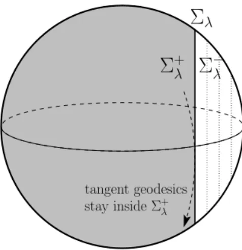
A typical example of such oriented pseudo-convex foliation without boundary is given in Figure 2.
By a classical argument, we may state a global version of Theorem 6.3 as follows. Theorem 6.5. Let Ω be a smooth compact manifold (with or without boundaries) and
let ω ⊂ Ω be an open set. Assume that there exists an oriented pseudo-convex foliation without boundary (Σλ)λ∈[0,1)of Ω in the sense of Definition 6.4. Also assume that Σ+0 ⊂ ω
and ω∪(∪λ∈[0,1)Σ+λ )
covers Ω up to a set of zero measure.
Let b, c and d be bounded coefficients. Assume that z is a global mild solution of
{
∂tt2z = ∆z + b(x, t)∂tz + c(x, t).∇z + d(x, t)z (x, t)∈ Ω × R
z|ω(x, t) = 0 (x, t)∈ ω × R
with any suitable boundary conditions on ∂Ω such that the wave equation is well-posed and where ∆ is the Laplace-Beltrami operator related to Ω.
Then z ≡ 0 everywhere.
Proof: We will show that z(·, t = 0) vanishes in ω∪Σ+λ, for all λ∈ [0, 1), which shows that
z(t = 0)≡ 0 and thus that z ≡ 0 due to the uniqueness properties of the wave equation.
By assumption, z ≡ 0 in Σ+0 ⊂ ω. Let λ0 ∈ (0, 1) and let hα,T(t) = α(1− t2/T2). We
consider the family of surfaces t ∈ [−T, T ] 7→ Σhα,T(t) which is locally parametrized by functions (x, t)7→ ψhα,T(t)(x). Notice that it is a smooth family of smooth surfaces since
Σ
λΣ
+λΣ
−λtangent geodesics stay inside Σ+λ
Figure 2: A oriented pseudo-convex foliation without boundary in the sphere S2. The surfaces Σλ forms a smooth family of vertical circles inside a hemisphere and Σ+λ and
Σ−λ are respectively the large and the small spherical caps. The geodesics beings the great circles, the ones which are tangent to a surface Σλ stay inside Σ+λ.
due to Assumption (i) of Definition 6.4. Also notice that the larger is T , the smaller are the derivatives of these functions with respect to t. By assumption, each function
x7→ ψλ(x) is non-characteristic and strongly pseudo-convex as a function independent of
t. By compactness, there exists T large enough such that (x, t)7→ ψhα,T(t)(x) defines local surfaces which are non-characteristic and pseudo-convex for all α∈ [0, λ0] and t∈ [−T, T ]. The parameter T is fixed in the remaining part of the proof and we may omit it in the notations.
Notice that, for any α, the family of set t∈ [−T, T ] 7→ Σ+hα(t) starts inside ω at t =−T and finishes inside ω at t = T . Moreover, for any small α, these sets always stay inside ω where z vanishes. Assume that there exist (x, t) and α∈ [0, λ0] such that x∈ Σ+hα(t) and
z(x, t)̸= 0. We set
α0= min{α ∈ (0, λ0] , ∃t ∈ [−T, T ], ∃x ∈ Σ+hα(t) such that z(x, t)̸= 0} . (6.4) By continuity, we know that z(x, t) = 0 for all x ∈ Σ+h
α0(t). Moreover, there exists
t0 ∈ (−T, T ) and x0 ∈ Σhα0(t0) such that z is not identically zero in any neighborhood of
(x0, t0). Indeed, otherwise, by compactness, we may extend the set where z vanishes and contradict (6.4).
To conclude, it remains to use the local unique continuation property of Theorem 6.3 at (x0, t0) with the time-space surface defined by (x, t)7→ ψhα0(t)(x). The continuation im-plies that z vanishes near (x0, t0) which contradicts the construction. Thus, z(x, t) = 0 for all t∈ [−T, T ] and x ∈∪αΣ+hα(t). In particular z(·, t = 0) ≡ 0 in∪αΣ+hα(0) =∪λ≤λ0Σ+λ. Since these arguments hold for all λ0< 1 and since ω∪λ∈[0,1)Σ+λ is Ω up to a set of
mea-sure zero, we have that z(·, t = 0) ≡ 0 in Ω. Well-posedness of the linear wave equation
concludes that z≡ 0 everywhere. □
Notice that, as it is stated, this unique continuation result needs an infinite time to be efficient, where Theorem 6.1 only need a finite explicit time. In fact, a careful look to the proof shows that a finite time is sufficient once we know that the family of surface is pseudo-convex and non-characteristic in a uniform way. However, such a bound of
convexity is difficult to obtain in general cases and may be even impossible as for the example studied in Section 7.
A typical example of application is given in Figure 2: if Ω is a sphere and ω covers more than an hemisphere, then if z is a global solution of a linear wave equation which vanishes in ω for all times, then z≡ 0. Notice that, in this case, the family of surfaces is uniformly pseudo-convex and the unique continuation holds in fact in finite time even if z is not a global in time solution.
6.3 Unique continuation through pseudo-convex surfaces with boundary The case where the pseudo-convex surfaces Σλ meet the boundary ∂Ω is more involved.
Theorem 6.3 has been generalized to this case by Tataru (see [41, 42, 43]). The boundary conditions are more difficult to describe geometrically, so we will only deal here with the case of flat geometry, that is g(x, ξ) =|ξ|2, and the case of Dirichlet boundary condition. Definition 6.6. A family of surfaces (Σλ)λ∈[0,1) is an oriented pseudo-convex foliation
with boundary in a flat manifold Ω if:
(i) the family of surfaces is smooth in the sense that it is locally described as level sets {x, ψλ(x) = 0} where (x, λ) 7→ ψλ(x) is a local smooth function with ∇xψλ ̸= 0.
(ii) each surface is globally oriented in the sense that there exist disjoint sets Σ±λ such that locally {x ∈ Ω, ±ψλ(x) > 0} ⊂ Σ±λ and such that Ω = Σ−λ ∪ Σλ∪ Σ+λ.
(iii) for each λ, (x, t)7→ ψλ(x) is pseudo-convex in the sense of definition 6.2 as a function
independent of t. Equivalently, Σ−λ is locally strictly convex in a neighborhood of its boundary: the tangent space to Σλ at x0 is locally included in Σ+λ, x0 excepted.
(iv) if a surface Σλ meet ∂Ω at x, then ∂νψλ(x) < 0. Equivalently, the angle formed by
Σλ and ∂Ω in the region Σ−λ is strictly less than π/2.
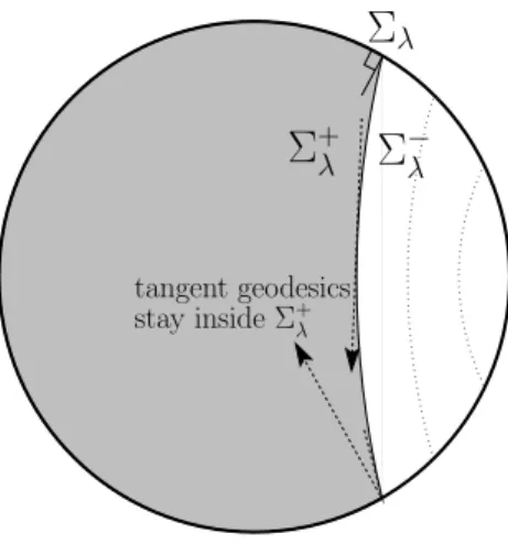
A typical example of such oriented pseudo-convex foliation with boundary is given in Figure 3. Notice that the condition at the boundary is consistent with the one inside the domain. Indeed, the geodesics are straight lines which bounce at the boundary according to Newton’s laws. Geometrically, we ask that any geodesic either crosses Σλ in a transversal
way, or stay locally inside Σ+λ.
By the same arguments as the ones in the proof of Theorem 6.5 and using the result of Tataru, we obtain a global unique continuation result.
Theorem 6.7. Let Ω⊂ Rd be a compact domain and let ω ⊂ Ω be an open set. Assume that there exists an oriented pseudo-convex foliation (Σλ)λ∈[0,1) of Ω in the sense of
Defi-nition 6.6. Also assume that Σ+0 ⊂ ω and ω ∪(∪λ∈[0,1)Σ+λ )
covers Ω up to a set of zero measure.
Let b, c and d be bounded coefficients. Assume that z is a global mild solution of
∂tt2z = ∆z + b(x, t)∂tz + c(x, t).∇z + d(x, t)z (x, t)∈ Ω × R z|∂Ω(x, t) = 0 (x, t)∈ ∂Ω × R z|ω(x, t) = 0 (x, t)∈ ω × R Then z≡ 0 everywhere.
A typical example of application is given in Figure 3: if Ω is a disk and ω covers more than half of the boundary, then if z is a global solution of a linear wave equation which vanishes in ω for all times, then z≡ 0.
Σ
+λΣ
−λΣ
λtangent geodesics stay inside Σ+λ
Figure 3: A oriented pseudo-convex foliation with boundary in the disk. The surfaces Σλ
forms a smooth family of curves inside a semidisk. The surfaces Σ−λ are strictly convex and the angle formed by Σλ and the boundary of the disk is less than π/2 on Σ−λ side.
The geodesics are straight lines bouncing at the boundary according to Newton’s laws. The ones which are tangent to a surface Σλ stay inside Σ+λ.
6.4 Proof of Theorem 1.2
Theorem 1.2 is then a direct consequence of the unique continuation results stated in this Section: Proposition 3.5 and Theorems 6.5 and 6.7 imply Theorem 1.2.
7
Application 2: the peanut of rotation
We consider in this section the example of the peanut of rotation: a two-dimensional manifold where a central part is equivalent to the cylinder {x = (y, θ) ∈ (−1, 1) × S} endowed with the metric g(y, θ) = dy2+ cosh2(y)dθ2 (see Figure 1). The damping γ is assumed to be positive, except in a part x∈ (−ℓ, ℓ) of the central part (ℓ ∈ (0, 1)). The decay of the linear damped wave semigroup has been established in [11] and [38].
Theorem 7.1. Christianson, Schenck, Vasy & Wunsch, 2014.
In the setting of the peanut of rotation, there exist two positive constants C and λ such that the semigroup eAt satisfies
∥eAtU
0∥X ≤ Ce−λ √
t∥U
0∥D(A) .
The decay rate of Theorem 7.1 obviously satisfies (1.4) and (1.5). Thus, once the unique continuation property is obtained, Proposition 3.5 yields the conclusion of Theorem 1.1 for the framework of the peanut of rotation. To obtain the unique continuation property, we will apply Theorem 6.5 with the family of pseudo-convex surfaces shown in Figure 4. Applying Theorem 1.2 and the ideas of Proposition 1.3, we obtain the following result. Theorem 7.2. Consider the damped wave equation (1.1) in the framework of the peanut
of rotation introduced above. Let α > 0 and f satisfying (1.2) and (1.3). Then, any solution u of (1.1) satisfies
∥(u, ∂tu)(t)∥H1
Σλ Σλ
Σ+λ Σ−λ Σ+λ
y = 0
Figure 4: An oriented pseudo-convex foliation without boundary of the central part of the
peanut. Each surface Σλ consists in two vertical circles, the set Σ−λ being the interior part
surrounded by these circles. Since the central part of the peanut is negatively curved, the geodesics tangent to the vertical circles stay in the exterior domain Σ+λ. Notice that the set Σ0 consists in both exterior disk and the disks Σλ get closer to x = 0 when λ get closer
to 1. Thus, the central circle x = 0 is not included in∪λ∈[0,1)Σ+λ but this is not important since this set is of zero measure.
Moreover, for any R and σ∈ (0, 1], there exists CR,σ such that, for any solution u with
U0∈ Xσ,
∥(u0, u1)∥H1+σ×Hσ ≤ R =⇒ ∥(u, ∂tu)(t)∥H1
0×L2 ≤ CR,σe
−σ˜λ√t
where ˜λ is the linearized rate given in Lemma 4.2.
Proof: Let us first formally check that the family of disks introduced in Figure 4 is
a suitable pseudo-convex foliation without boundary. We use the cylindrical coordinates
x = (y, θ)∈ (−1, 1)×S with associated tangent variables ξ = (ζ, Θ). By symmetry, we only
consider the right-hand-side circles which are defined by ψλ(x) = 0 with ψλ(x) = y−(1−λ).
The circle Σ0 corresponding to y = 1 is in the interior of the region ω where the damping is positive. When λ get closer to 1, the circle Σλ get closer to y = 0. We are obviously in
the setting of Definition 6.4 and thus of Theorem 1.2, except maybe for the assumption of strong pseudo-convexity. We already give a geometrical insight of this assumption, but let us check it formally.
The local metric is given by g(y, θ) = dy2+ cosh2(y)dθ2. The Laplace-Beltrami oper-ator is thus given by
∆g = ∂yy2 + 2 tanh(y)∂y+
1 cosh2(y)∂
2
θθ .
The principal part of the wave operator is then
p(y, θ, t, ζ, Θ, τ ) =|ζ|2+ 1 cosh2(y)|Θ| 2− |τ|2 . Thus Hp(ψλ) = 2ζ and Hp2(ψλ) = 4 sinh(y) cosh(y)3|Θ| 2 .
The pseudo-convexity condition is then checked. Indeed, if Hp(ψλ) = 0 then ζ = 0 and
since ξ = (ζ, Θ) must be non-zero, we must have Θ̸= 0. As ψλ(y, θ) = 0 with λ∈ [0, 1),
we have y > 0 and thus Hp2(ψλ) > 0. Looking carefully to the computations, one notes
that, in fact, we only need that the radius cosh(y) of the cylindrical part is increasing for