HAL Id: hal-00624814
https://hal.archives-ouvertes.fr/hal-00624814
Submitted on 19 Sep 2011
HAL is a multi-disciplinary open access
archive for the deposit and dissemination of sci-entific research documents, whether they are pub-lished or not. The documents may come from teaching and research institutions in France or abroad, or from public or private research centers.
L’archive ouverte pluridisciplinaire HAL, est destinée au dépôt et à la diffusion de documents scientifiques de niveau recherche, publiés ou non, émanant des établissements d’enseignement et de recherche français ou étrangers, des laboratoires publics ou privés.
Full-Field Birefringence Imaging by Thermal-Light
Polarization-Sensitive Optical Coherence Tomography.
II. Instrument and Results
Julien Moreau, V. Loriette, A.C. Boccara
To cite this version:
Julien Moreau, V. Loriette, A.C. Boccara. Full-Field Birefringence Imaging by Thermal-Light Polarization-Sensitive Optical Coherence Tomography. II. Instrument and Results. Applied optics, Optical Society of America, 2003, 42 (19), pp.3811-3818. �10.1364/AO.42.003811�. �hal-00624814�
Full-field birefringence imaging by thermal-light
polarization-sensitive optical coherence
tomography.
II.
Instrument and results
Julien Moreau, Vincent Loriette, and Albert-Claude BoccaraWe describe an instrument for measuring the magnitude of birefringence of tomographic images and the principal directions of axes that uses thermal-light polarization-sensitive optical coherence tomography. The instrument permits full-field measurements with an axial resolution of 1.5m and a transverse resolution limited by diffraction. We obtained a sensitivity of 84 dB, limited by shot noise, when we integrated the signal for 1 s. We verified the validity of the measurement by measuring the birefrin-gence of a variable phase shifter. We present typical results obtained with optical samples. © 2003 Optical Society of America
OCIS codes: 110.4500, 120.5060, 260.1440.
1. Introduction
Optical coherence tomography 共OCT兲 is an attrac-tive technique for obtaining information about bur-ied structures with high spatial resolution. OCT is oriented mainly toward the study of diffusive sam-ples, but it can be used as well for testing transpar-ent samples with low optical contrast. In this case polarization-sensitive OCT, which brings the ad-vantages of dark-field microscopy, proves to be an effective technique for revealing structures that otherwise would hardly be detectable.1–9 The
com-bination of a polarization-sensitive instrument with a broadband source allows one to obtain polarization-dependent information with micrometer-scale res-olution in three dimensions. With a CCD array, full-field microscopy is possible.10 –12 The
coher-ence length of the broadband source determines the axial resolution of the instrument, so microscope objective lenses with large depths of field or low numerical apertures can be used without spoiling the axial resolution. Unless one uses immersion
objectives and samples with low index variations, the use of low-numerical-aperture objectives is obligatory when one tests samples that exhibit large index changes because aberrations inside the sample put severe limitations on the depth that can be probed. However, the use of a broadband source raises a major technical problem: Although achro-matic polarizers can be manufactured easily, mak-ing a fairly achromatic phase-shiftmak-ing component is a difficult task. The most common achromatic phase-shifting component is the Fresnel rhomb. Standard commercially available Fresnel rhombs exhibit phase errors of a few degrees over a span of a few hundred nanometers. Unfortunately the standard design of Fresnel rhombs makes them un-suitable for OCT microscopy because they shift the emerging beam laterally and are highly sensitive to misalignment. The use of multilayer phase-shifting plates permits the problem of beam shift to be overcome, but phase-shifting plates are far less efficient than rhombs in the blue part of the spec-trum, and their performance varies greatly from one manufacturer to the other. The present au-thors have chosen to use achromatic quarter-wave plates, chiefly because of their ease of use, although, for some experimental configurations, this choice is made to the detriment of accuracy and sensitivity. In Section 2 of this paper we describe the experi-mental arrangement, and in Section 3 we discuss its performance. We focus on elimination of the spu-rious signal induced by phase errors in the
quarter-The authors are with the E´ cole Supe´rieure de Physique et Chimie Industrielles de la Ville de Paris, Laboratoire d’Optique Physique, Centre National de la Recherche Scientifique Unite´ Pro-pre de Recherche 5, 10 rue Vauquelin, 75005 Paris, France. V. Loriette’s e-mail address is [email protected].
Received 13 September 2002; revised manuscript received 28 January 2003.
0003-6935兾03兾193811-08$15.00兾0 © 2003 Optical Society of America
wave plates. In Section 4 we present some results for multilayer optical samples.
2. Experimental Arrangement
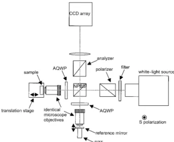
The experimental arrangement is sketched in Fig. 1. The instrument is based on a Linnik interfer-ence microscope, i.e., a Michelson interferometer with a microscope objective lens in each arm. The reference surface should have topographic features much smaller than the sample, and to optimize the contrast its reflectance should be as close as possi-ble to the reflectance of the sample. Uncoated glass, which has a low reflection factor of⬃4% and can be superpolished, is a good choice when one is testing biological or transparent optical samples. Light is emitted by a xenon lamp with 300-nm bandwidth centered about 800 nm. It is polarized with a Glan–Taylor polarizer that has an extinction ratio of 2 ⫻ 10⫺5. The beam is divided by a non-polarizing beam-splitter cube. Each arm contains an achromatic quarter-wave plate共Newport Corpo-ration Model ACWP兲 and a 20⫻, microscope objec-tive with a N.A. of 0.4 共Olympus 20⫻ plan achromat兲. The emerging light is collected by a CCD array 共256 ⫻ 256 pixel, 8-bit, maximum 200-Hz readout frequency; Dalsa Semiconductors Model CAD-1兲 after it has passed through a thin plate polarizer with an extinction ratio of 4⫻ 10⫺5. The plate polarizer is fixed upon a motorized rota-tion stage to permit angular posirota-tioning with a pre-cision of 0.17 mrad. Both reference mirror and sample are fixed upon motorized translation stages. The reference is attached to a piezoelectric actuator oscillating at 45 Hz, and the sample is translated with a 74-nm step motorized translation stage. The amplitude of piezo-oscillation can be adjusted to produce a particular modulation depth. The pi-ezoactuator driver and the CCD are phase locked by two waveform generators 共Hewlett-Packard Model 33120A兲. The total acquisition time depends on
the number of averages for each position of the sample and on the total volume scanned; a good order of magnitude is 4 s兾section for a 100-image average.
3. Setup and Measurement Procedure
The orientations of the various polarization compo-nents are adjusted by use of extinction configura-tions. At the end of this step the polarizer is oriented to produce a P-polarized field incident upon the beam splitter. The quarter-wave plate in the sample arm is oriented such that its fast axes make an angle of 45° with the P axis, and the quarter-wave plate in the reference arm is oriented at 11°. These values allows the signal-to-noise ra-tio to be maximized, as explained below. During this step of the setup the CCD is replaced by a silicon photodetector for better sensitivity. With digital waveform generators, both modulation depth and phase are adjusted independently by use of the method discussed in Ref. 13. By measuring four images with a tilted nonbirefringent test sam-ple and calculating S2共P兲–S4共P兲 we can adjust the
modulation phase to 兾4. By making the fringes disappear at the center of the interferogram, as shown in Fig. 2, we can fix the modulation depth close to its theoretical value of 2.0759 rad with an estimated precision of 98%. Once the modulation parameters are fixed, the nonbirefringent test sam-ple is replaced by the samsam-ple that we wish to study. We then record two sets of four images兵Si共S兲, Si共P兲其,
i⫽ 1–4, acquired with two different orientations, S
and P, of the analyzer. For a given analyzer posi-tion the corresponding four images are acquired consecutively; each image is integrated during one quarter of the modulation period. This eight-image acquisition is performed for each position of the sample. We form four linear combinations:
⌺B共S兲⫽ ⫺S1共S兲⫹ S2共S兲⫹ S3共S兲⫺ S4共S兲, (1)
⌺A共S兲⫽ ⫺S1共S兲⫹ S2共S兲⫺ S3共S兲⫹ S4共S兲, (2)
⌺B共P兲⫽ ⫺S1共P兲⫹ S2共P兲⫹ S3共P兲⫺ S4共P兲, (3)
⌺A共P兲⫽ ⫺S1共P兲⫹ S2共P兲⫺ S3共P兲⫹ S4共P兲; (4)
Fig. 1. Schematic of the instrument described in this paper: NPBS, nonpolarizing beam-splitter cube; AQWPs, achromatic quarter-wave plates; PZT, piezoactuated translation stage.
Fig. 2. Procedure used to fix the value of␦0: interferograms with
and calculate birefringence magnitude ␦B, orienta-tion, and signal topography ␦zwith the formulas
tan2
冉
␦B 0冊
⫽ tan⫺2共2兲关⌰B⌺A共P兲兴2⫹ 关⌰A⌺B共P兲兴2 关⌰B⌺A共S兲兴2⫹ 关⌰A⌺B共S兲兴2 , (5) tan冉
2 ␦z 0冊
⫽⌰B⌺A共S兲 ⌰A⌺B共S兲 (6) tan共2兲 ⫽⌰A⌰B关⌺A 共S兲⌺ B共P兲⫺ ⌺A共P兲⌺B共S兲兴 ⌰A 2⌺ B共S兲⌺B共P兲⫹ ⌰B 2⌺ A共S兲⌺A共P兲 , (7)where, knowing the apparent spectrum of the source, we calculate ⌰A and ⌰B, and 0 is an equivalent
wavelength of the polychromatic source.
4. Results
We calibrated our instrument by inserting a Babinet compensator into the sample arm between the quarter-wave plate and the microscope objective. We generated a well-defined birefringence signal with known axial directions and varied its amplitude from⫺兾2 to ⫹兾2. Figure 3 shows the measured birefringence as a function of the true retardation imposed by the compensator. The best linear fit is shown共solid line兲; its coefficient of linear regression is 0.99985, slope is 0.993⫾ 0.005, and intercept is ⫺3 ⫾ 5 mrad, demonstrating the good agreement of the measurement with the true values. However, it must be noted that to obtain this result we found it necessary to take into account the imperfections of the quarter-wave plates. This correction is de-scribed in Section 5 below.
We validated our setup with a multilayer optical coating sample whose structure is sketched in Fig. 4. For an optical system with a scattering specification level of a few parts in 106 共laser gyros or
interfero-metric detectors of gravitational waves14,15兲, point
de-fects inside the multilayer coating are a major source of loss. Knowing the locations of these scattering
defects, and furthermore using a nondestructive tech-nique, will help in finding the source of contamina-tion. This detection cannot be made by use of a tomographic image of the reflectance of the structure because the specular light from the interfaces would mask the small signal coming from the defect. How-ever, if the scattering defect is nonspherical, it can change the polarization of the incident light. There-fore, in a tomographic image of the birefringence the point defect will appear as a bright spot in a dark field, as the interfaces are not birefringent. Our sample is an infrared interference coating designed for a CO2 laser 共 ⫽ 10.6 m兲, with five layers of
alternate high- and low-index dielectric material de-posited upon a ZnSe substrate. The layers are al-ternately half-wave and quarter-wave plates. Figure 5 shows the interferogram envelope: ⍀共z兲,13
which in this case is similar to the classic OCT
to-Fig. 3. Relation of estimated to true retardation of a Babinet compensator: squares, uncorrected data; crosses, data corrected for quarter-wave plate error following to Eq.共15兲.
Fig. 4. Schematic of the multilayer optical coating mirror used as a sample.
Fig. 5. Classic OCT tomography cut of the multilayer. Six in-terfaces can be distinguished.
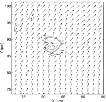
mography signal. It must be noted that the scale of the Z axis is given by the translation of the sample upon its motorized stage. To obtain true optical thickness values one should correct the Z scaling by an obliquity factor that depends on the objective’s N.A. and on the sample’s index of refraction. The axial resolution of our instrument enables us to re-solve the six interfaces. We made a three-dimensional birefringence map of this mirror 共60 images; step, 0.4m兲 to enable us to detect the pres-ence of point defects inside the structure. Figures 6 and 7, respectively, show XY cuts of the magnitude and direction of the birefringence axes about such defects. Figures 8 and 9, respectively, show XZ and
YZ cuts. In these cuts the noise was measured to be
2.9⫻ 10⫺4rad. Figure 7 shows a measurement of the direction of the birefringence axes in the region where the defect was detected. To ensure quantita-tive measurement we evaluated the birefringence only when ⍀ took a significant value. A defect in birefringence can be seen and precisely located on the second interface. Its size is equal to or less than the resolution of our instrument in three dimensions. The spurious birefringence signal coming from the interfaces共⬃0.1 rad兲 is due to a retardation error of the achromatic quarter-wave plate 共see Subsection 5.D below兲. The time needed to acquire a complete three-dimensional map of a sample depends on the number of XY cuts as well as on the number of images averaged at each position of the sample. In the mea-surement presented, the sample was moved to 60 different Z positions, and an average of 400 se-quences was performed at each position, so the total number of images acquired was 60⫻ 8 ⫻ 400. The time needed for the sample to move from one position to the next was 200 ms, and the total acquisition time was 17 min.
Fig. 6. En face birefringence image of the multilayer second
in-terface on which a defect is visible: XY cut, 0.7m ⫻ 0.7 m
resolution. The noise in this image is estimated to be 2.9⫻ 10⫺4 rad.
Fig. 7. Direction of the birefringence axes in the region about the defect on the multilayer second interface; XY cut. The contour lines indicate the locations of the birefringent structures.
Fig. 8. High-resolution共0.7 m ⫻ 1.5 m, lateral ⫻ axial兲 bire-fringence image of the multilayer; XZ cut; same noise level as in Fig. 6. Dashed lines, positions of the six interfaces.
5. Performance and Limitations
A. Resolution and Position Accuracy
The axial resolution in air is evaluated with a single interferogram recorded by use of a mirror sample. From the measurement presented in Fig. 10 one can find the best Gaussian envelope of the interferogram and estimate the full-width at half-maximum. We found axial resolution⌬z⫽ 1.5 m in air. The axial
resolution is limited by the apparent spectrum width of the light source presented in Fig. 11 共i.e., which takes into account the spectral response of the CCD array and of the optical components兲 and by uncom-pensated dispersion inside the interferometer and in-side the sample. The uncompensated dispersion can
in principle be corrected if one knows the dispersion curves and the thicknesses of the various optical el-ements and sample. The accuracy of the axial posi-tion depends on the algorithm that uses one to find the position of the maximum of the interferogram envelope and is limited by the axial step size of the sample displacement. In our setup the displace-ment step size is 74 nm, which can be taken as a good order of magnitude of the accuracy of the axial posi-tion.
The lateral resolution in air is limited by diffraction and depends on the objective lenses that are used. We use an optical scheme in which each pixel of the CCD array receives the image of a cross section of the sample approximately equal to the diffraction spot size, so the accuracy of the lateral position is equal to the resolution. When better lateral accuracy is re-quired, expanding imaging optics can be added such that the diffraction spot is imaged on more than a single pixel.
B. Maximum Detectable Birefringence
The short coherence length limits the maximum mag-nitude of birefringence that can be detected: If the retardation induced by the sample is larger than the coherence length of the source, then, after interaction with the sample, the two eigenstates of polarization will lose their mutual coherence and the field return-ing from the reference arm will become a superposi-tion of two orthogonally polarized incoherent fields. The maximum value of the birefringence that can be measured is max共␦B兲 ⫽ ⌬z, or, expressed in terms of
phase retardation and using the equivalent wave-length of the source,
max共兲 ⫽ 2⌬z 0
. (8)
In our setup this value is⬃3.
C. Sensitivity
The performance of the instrument is limited by two factors, residual noise and imperfections and misori-entation of the polarizing components, especially the quarter-wave plates and the beam-splitter cube. The former puts an upper limit on sensitivity and the latter, together with uncertainties in the modulation parameters, degrade measurement precision. The fundamental sensitivity limits of the instrument are discussed in depth in the paper by Dubois.16 We
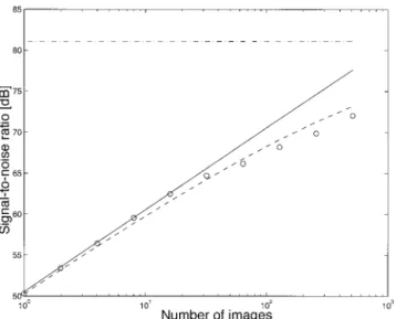
measured the signal-to-noise ratios 共SNRs兲 of indi-vidual images and found that they are shot-noise limited up to an integration duration of 20 s. During 1-s integration we measured a SNR of 70 dB; the theoretical value of the shot-noise-limited SNR for a 13⫻ 104charge per pixel CCD is 73 dB. Usually in OCT-related papers the SNR is given as a minimum sample reflectance, measured with a glass reference surface.16 In that case a correction equal to⫺20 ⫻
log10共公Rglass兲 ⫽ 14 dB is added to the SNR value,
which in the study reported here increases to 84 dB. When the duration of integration becomes large,
Fig. 10. Measured axial response of the system and best Gauss-ian envelope. The FWHM is 1.5m.
Fig. 11. Spectrum of the light source used in the experiment as a function of wavelength.
other sources of noise, possibly mechanical, acoustic, and thermal, become dominant.
The shape of the measured sensitivity-versus-time plot presented in Fig. 12 suggests that this technical noise may exhibit an f⫺1frequency dependency, and its presence places an upper limit of 81 dB共95 dB in terms of minimum reflectance with an uncoated glass reference兲 on the SNRs of individual images. How-ever, we are interested not in the SNRs of individual images but in the SNR of the birefringence measure-ment. The way to compute the SNR of the birefrin-gence measurement, SNR共兲, starting from the SNR of individual images, SNR共S兲, is straightforward but lengthy, and we simply outline it here. We start our calculation by assuming that each image exhibits the same average value and noise level as the other im-ages and that the noise of the various imim-ages is un-correlated. These assumptions allow to calculate the SNRs of the various combinations of⌺A共S兲,⌺A共P兲,
⌺B共S兲, and⌺B共P兲, using Eqs.共1兲–共4兲, and then the SNR
of the birefringence measurement, using Eq. 共5兲. There is a simple relation between the SNRs of indi-vidual images SNR共S兲 and the SNR of the birefrin-gence measurement SNR共兲 that depends on the magnitude of the birefringence and on the orientation of the quarter-wave plate in the reference arm:
SNR共兲 ⫽ SNR共S兲 ⫻ g共, 兲, (9) where g is a known function of, , and the modula-tion amplitude. The plot of g in Fig. 13, calculated for⌰A⫽ ⌰B, shows that the value of that gives the highest SNR for the broadest range of is ⬃11° 关the optimal value is 22.5° only when one is interested in measuring tan共兾2兲兴. Figure 14 is a plot of g共, 11°兲, which shows that SNR共兲 is roughly ten times less than SNR共S兲. We thus estimate the maximum SNR for a birefringence measurement to be 61 dB共50 dB for 1-s integration兲.
D. Precision
The most important limitation on instrument preci-sion comes from the various imperfections of the op-tical components, in particular, their behavior with respect to polarization. The requirement of achro-maticity is scarcely achievable in polarization compo-nents. For polarizers it appears as a poor extinction factor; for phase-shifting components, as spurious wavelength dependent retardation. To eliminate any displacement of the image on the CCD when we rotate the analyzer, we have to use a thin polarizer with an extinction two times larger than one could obtain with a Glan-type polarizer. Then, as was found experimentally, coupling of polarization states can occur inside the beam-splitter cube if the cube is slightly misaligned with respect to the axes of the two arms. It is rather difficult to overcome this problem because it does not show in pure intensity images and is hardly distinguishable a priori for misorientations of the polarizer or the analyzer. The optical compo-nents that cause the largest imperfections are the two achromatic quarter-wave plates, as we empha-sized above. A simple calculation can be performed for a monochromatic source in the presence of spuri-ous retardation of ␦Q waves in the quarter-wave
Fig. 12. Image SNR as a function of the number of images aver-aged. Circles, measurements; solid line, shot-noise limit; dashed curve, estimate of the SNR if an f⫺1noise source is present; hor-izontal dashed– dotted line, SNR limit imposed by the f⫺1noise.
Fig. 13. Value of g as a function of birefringence magnitude and orientation of the quarter-wave in reference arm.
Fig. 14. Value of g as a function of birefringence magnitude for ⫽ 11.26°.
plates. In this case the Jones matrix of the quarter-wave plates reads as
MQ⫽
冤
exp冋
i冉
4⫹ ␦Q冊册
0 0 exp冋
⫺i冉
4⫹ ␦Q冊册
冥
. (10)The apparent birefringence of the sample,app,
cal-culated with the standard equation that is valid for the monochromatic source, is related here to the true value of the birefringence by
tan2
冉
app 2冊
⫽ sin2共兾2兲 ⫹ h共, , ␦ Q兲 cos2共兾2兲 ⫺ h共, , ␦Q兲 , (11) with h共, , ␦Q兲 ⫽ 关cos2共兾2兲⫺ sin2共2兲sin2共兾2兲兴sin2共2␦ Q兲
⫺ sin共兲sin共2兲cos共4␦Q兲. (12)
The true value of␦Qis an unknown function of
wave-length that depends on the structure of the quarter-wave plate used. Its apparent value can nevertheless be measured by use of a nonbirefringent sample; then the apparent birefringence is
tan2
冉
app 2冊
⫽ sin2共2␦Q兲 1⫺ sin2共2␦ Q兲 ⬇ 4␦Q 2 1⫺ 4␦Q2 . (13) We found experimentally that ␦Q ⫽ 25 mrad; thevalue of h can then be estimated from the apparent values of app and app. It is worth noting that h
does not depend on topography␦z. To calculate h we
need the sign of sin共app兲 ⫻ sin共2app兲. It can be
found because, when 0ⱕ ⱕ 兾4, one combination of the four signals⌺A
S ,⌺B S ,⌺A P , and⌺B P
has the same sign:
sign关sin共兲sin共2兲兴 ⫽ sign关⌺A共P兲⌺B共S兲⫺ ⌺A共S兲⌺B共P兲兴,
0ⱕ ⱕ 兾4. (14)
The true value of can then be estimated by tan2
冉
2
冊
⬇ cos2共app兾2兲 ⫺ h共app,app,␦Q兲
sin2共app兾2兲 ⫹ h共app,app,␦Q兲
. (15) The calibration plot of Fig. 3 was obtained with rela-tion共15兲.
6. Conclusion
We have constructed a polarization-sensitive Linnik-type interference microscope that works with a ther-mal light source. Our system uses full-field illumination with sinusoidal phase modulation and four integrating buckets. This system can produce
en face共x–y兲 tomographic images of the birefringence
with a resolution of 1m in the transverse direction and 1.5m in the axial direction without scanning. Quantitative measurements can be obtained for bi-refringence from 0.1 to 3 rad; these limits are fixed
by the imperfections of the achromatic quarter-wave plates and the coherence length of the source. The maximum sensitivity of our setup, in terms of mini-mum detectable sample reflectance, was found to be 95 dB 共84 dB for 1-s integration兲 for an individual image and⬃61 dB 共⬃50 dB for 1-s integration兲 for a birefringence measurement. We used our system as a dark-field microscope to detect and localize micrometer-sized defects inside a multilayer optical coating infrared mirror. Our primary interest was to gain a better understanding of the locations of scattering defects in multilayer optical coatings and therefore to determine the sources of contamination. Nevertheless, we are also currently investigating ways in which to use our microscope to study biolog-ical samples.
The authors thank Arnaud Dubois and Laurent Vabre for helpful discussions.
References
1. J. F. de Boer, T. E. Milner, M. J. C. van Gemert, and J. S. Nelson, “Two-dimensional birefringence imaging in biological tissue by polarization-sensitive optical coherence tomogra-phy,” Opt. Lett. 22, 934 –936共1997兲.
2. J. F. de Boer, S. M. Srinivas, A. Malekafzali, Z. Chen, and J. S. Nelson, “Imaging thermally damaged tissue by polarization sensitive optical coherence tomography,” Opt. Express 3, 212– 218共1998兲, http:兾兾www.opticsexpress.org.
3. M. J. Everett, K. Schoenenberger, B. W. Colston, Jr., and L. B. Da Silva, “Birefringence characterization of biological tissue by use of optical coherence tomography,” Opt. Lett. 23, 228 –230 共1998兲.
4. K. Schoenenberger, B. W. Colston, Jr., D. J. Maitland, L. B. Da Silva, and M. J. Everett, “Mapping of birefringence and thermal damage in tissue by use of polarization-sensitive optical coherence tomography,” Appl. Opt. 37, 6026 – 6036 共1998兲.
5. J. F. de Boer, T. E. Milnerand, and J. S. Nelson, “Determina-tion of the depth-resolved Stokes parameters of light backscat-tered from turbid media by use of polarization-sensitive optical coherence tomography,” Opt. Lett. 24, 300 –302共1999兲. 6. G. Yao and L. V. Wang, “Two-dimensional depth-resolved
Mueller matrix characterization of biological tissue by optical coherence tomography,” Opt. Lett. 24, 537–539共1999兲. 7. C. E. Saxer, J. F. de Boer, B. H. Park, Y. Zhao, Z. Chen, and
J. S. Nelson, “High-speed fiber-based polarization-sensitive op-tical coherence tomography of in vivo human skin,” Opt. Lett.
25, 1355–1357共2000兲.
8. C. K. Hitzenberger, E. Go¨tzinger, M. Sticker, M. Pircher, and A. F. Fercher, “Measurement and imaging of birefringence and optic axis orientation by phase resolved polarization sensitive optical coherence tomography,” Opt. Express 9, 780 –790 共2001兲, http:兾兾www.opticsexpress.org.
9. J. E. Roth, J. A. Kozak, S. Yazdanfar, A. M. Rollins, and J. A. Izatt, “Simplified method for polarization-sensitive optical co-herence tomography,” Opt. Lett. 26, 1069 –1071共2001兲. 10. P. de Groot and L. Deck, “Surface profiling by analysis of
white-light interferograms in the spatial frequency domain,” J. Mod. Opt. 42, 389 – 401共1995兲.
11. E. Beaurepaire, A. C. Boccara, M. Lebec, L. Blanchot, and H. Saint-Jalmes, “Full-field optical coherence microscopy,” Opt. Lett. 23, 244 –246共1998兲.
12. A. Dubois, L. Vabre, A.-C. Boccara, and E. Beaurepaire, “High-resolution full-field optical coherence tomography with a Lin-nick microscope,” Appl. Opt. 41, 805– 812共2002兲.
13. J. Moreau and V. Loriette, “Full-field birefringence imaging by thermal-light polarization-sensitive optical coherence tomog-raphy. 1. Theory,” Appl. Opt. 42, 3800 –3810共2003兲. 14. J. M. Mackowski, L. Pinard, L. Dognin, P. Ganau, B. Lagrange,
C. Michel, and M. Morgue, “Different approaches to improve the wavefront of low-loss mirrors used in the VIRGO gravita-tional wave antenna,” Appl. Surf. Sci. 151, 86 –90共1999兲.
15. J.-Y. Vinet, V. Brisson, S. Braccini, I. Ferrante, L. Pinard, F. Bondu, and E. Tournie´, “Scattered light noise in gravitational wave interferometric detectors: a statistical approach,” Phys. Rev. D 56, 6085– 6095共1997兲.
16. A. Dubois, “Phase-map measurements by interferometry with sinusoidal phase modulation and four integrating buckets,” J. Opt. Soc. Am. A 18, 1972–1979共2001兲.