Is the Heart Preadapted to Hypoxia?
Evidence from Fractal Dynamics of
Heartbeat Interval Fluctuations
at High Altitude (5,050 m)
M. MEYER, 1,3 A. RAHMEL, 3 C. MARCONI, 2 B. GRASSI, 2 J.E. SKINNER 4 AND P. CERRETELU 1,2 Ddpartement de Physiologic, CMU, Genive, Switzerland 1
lstituto di Tecnologie Biomediche Avanzate, CNR, Milano, Italy 2
Department of Physiology, Max Planck Institute for Experimental Medicine, Gi~ttingen, Germany s Cardiovascular Division, Torts Gap Laboratories, Bangor, PA, USA 4
Abstract--The dynamics of heartbeat interval time series over large time scales were studied by a modified random walk analysis introduced recently as Detrended Fluctuation Analysis. In this analysis, the intrinsic fractal long-range power-law correlation properties of beat-to-beat fluctuations generated by the dynamical system (i.e., cardiac rhythm gen- erator), after decomposition from extrinsic uncorrelated sources, can be quantified by the scaling exponent (o0 which, in healthy subjects, for time scales of ~ 104 beats is ~ 1.0. The effects of chronic hypoxia were determined from serial heartbeat interval time series of digitized twenty-four-hour ambulatory ECGs recorded in nine healthy subjects (mean age thirty-four years old) at sea level and during a sojourn at 5,050 m for thirty-four days (Ev- K2-CNR Pyramid Laboratory, Sagarmatha National Park, Nepal). The group averaged r exponent (+SD) was 0.99 + 0.04 (range 0.93 - 1.04). Longitudinal assessment of r in individual subjects did not reveal any effect of exposure to chronic high altitude hypoxia. The finding of ct - 1 indicating scale-invariant long-range power-law correlations (llf noise) of heartbeat fluctuations would reflect a genuinely self-similar fractal process that typically generates fluctuations on a wide range of time scales. Lack of a characteristic time scale along with the absence of any effect from exposure to chronic hypoxia on scaling properties suggests that the neuroautonomic cardiac control system is preadapted to hypoxia which helps prevent excessive mode-locking (error tolerance) that would restrict its functional responsiveness (plasticity) to hypoxic or other physiological stimuli.
Key Words---autonomic nervous system, cardiac rhythm, electrocardiography, heart rate, high altitude, non-linear dynamics, l/f noise, sealing properties
Introduction
ACUTE EXPOSURe to severe h y p o b a r i c h y p o x i a equivalent to that e n c o u n t e r e d on the s u m m i t o f Mt. E v e r e s t (8,846 m ) w o u l d rapidly b e detrimental to h u m a n subjects. In contrast, c h r o n i c exposure, i.e., p r o v i d e d sufficient time is a l l o w e d for a c c l i m a t i z a t i o n to the h y p o x i c e n v i r o n m e n t , would e n a b l e m a n to c l i m b m o u n t a i n s well a b o v e 8,000 m w i t h o u t s u p p l e m e n t a l o x y g e n . In order to c o p e with this extraordinary m u l t i - e n v i r o n m e n t a l
Address for Correspondence: Professor Michael Meyer, M.D., Ph.D., Department of Physiology, M a x Planck Institute for Experimental Medicine, Hermann-Rein-Stral3r 3, D - 37075 G6ttingen, Germany; E-Mail: meyer @exmda2.mpiem.gwdg.dc
10 ~ v r ~ E'r AL.
challenge of which hypoxia is the most important, substantial complex readjustments of the pulmonary, cardiovascular, and metabolic systems are known to occur, many of which are not completely understood (Banchero, 1987; Cerretelli, 1980; Cerretelli and Hoppeler, 1996; Ueda et al., 1992; Ward et al., 1990).
A primary component of the initial cardiovascular response to high altitude hypoxia is an increase in heart rate (Hughson et al., 1994; Malhotra et al., 1976; Richalet et al., 1988; Wolfel et al., 1994) which has been attributed to readjustment in the balance of the sympathetic and parasympathetic components of the autonomic nervous system. Evidence for an increased sympathetic neural activity has been derived by studies of plasma cat- echolamine levels (Mazzeo et al., 1991; Richalet et al., 1988; Wolfel et al., 1994; Young et al., 1991) and power spectral analysis of short-term heart rate variability (Farinelli et al., 1994; Hughson et al., 1994; Yamamoto and Hughson, 1991), but also the emergence of more complex nonlinear dynamics has been described (Lipsitz et al., 1995; Malconian et al., 1990; Schoene, 1982; Yamamoto et al., 1993).
The long-term variability of heart rate observed over a wide range of time scales with scale-invariant power-law characteristics (l/f noise) has recently been associated with the fractal scaling behavior and long-range correlation properties typically exhibited by dy- namical systems near a critical point of a phase transition, i.e., far away from equilibrium (Bak and Creutz, 1994; Peng et al., 1993b; 1995; Stanley, 1971). The fractal scaling exponent (r of normal twenty-four-hour heartbeat interval time series (about 104 beats) calculated by a novel algorithm
(Detrended Fluctuation Analysis, DFA)
was ~ 1.0, indicat- ing the presence of non-trivial long-range correlations (memory-like effects) while patients with congestive heart failure showed a significant deviation of the long-range correlation exponent from normal (~ 1.25). The physiological significance of the long-range power-law or l/f behavior of normal cardiac interbeat time series has not been established. The physiological advantage of a non-equilibrium dynamical system operating over a wide range of time scales, unlike a classic homeostatic process, may be attributed to its capacity to respond to external or environmental stimuli(plasticity)
while preserving a relative insensitivity to errors(error tolerance).
Hypothesis
In pursuit of this concept, we hypothesized that the normal intact heart, in terms of the intrinsic mechanisms controlling heart rate and its fluctuations, is
preadapted
to external stimuli such as hypoxia encountered during exposure to a hypobaric environment, i.e., high altitude. Unlike other systems of oxygen transport (e.g., pulmonary, blood, tissue) that, as a strategy of adaptation, undergo functional and structural changes, the mechanisms under- lying the control of heart rate would be expected to demonstrate lack of any adaptation to hypoxia. Specifically, we hypothesized that the fractal scaling properties of long-term heartbeat interval time series were unaffected by chronic exposure to high altitude hy- poxia. On the contrary, viz. rejection of the hypothesis, physiological adaptation, defined as a change of a physiological variable which reduces the strain imposed by stressful components of the environment, is known to be time-dependent and would be expected to elicit differential responses that rely on instantaneous strategies in the acute phase and on acclimatization in the chronic phase.FRACTAL DYNAMICS OF HEART RATE AT ALTITUDE 11
Objectives
The present analysis is mainly based on heartbeat interval time series obtained from twenty-four-hour Holter ECG recordings of normal Caucasian subjects and Himalayan Sherpas chronically exposed to high altitude hypoxia (5,050 m). The major objectives of the present study were: 1) to quantify the scaling exponent and correlation properties of non-stationary heartbeat interval time series over extended twenty-four-hour epochs and shorter four-hour day/nighttime subepochs; 2) to assess the stability or adaptive changes that would result from chronic exposure to a hypoxic environment, i.e., testing the hypoth- esis that the "fractal complexity" of heart rate dynamics remains essentially unchanged by hypoxia; and 3) to evaluate the mechanisms and physiological significance underlying the fractal complexity of heart rate dynamics.
Methods
Subjects
Nine Caucasian subjects (7 males, 2 females; mean age + SD, 33.7 + 4.6 years), all members of a medical high altitude expedition and trained in physiology, volunteered for the study. They were physically untrained and in their normal sedentary life engaged in laboratory work. From Milan, Italy (122 m a.s.1.) they were flown to Kathmandu, Nepal (1,350 m) and continued to Lukla (2,850 m), from where they trekked for six days to the Italian EvK2-CNR high altitude Pyramid Laboratory (Sagarmatha National Park, Khumbu Valley, Nepal, 5,050 m - 16,568 ft; Pb - 420 mmHg, Pro2 ~ 79 mmHg) located in the vicinity of the Everest Base Camp. Trekking consisted of several hours of walking per day at a moderate pace while carrying a light load. Two resting days, at 3,440 m and 4,243 m, were allowed for proper acclimatization and all subjects were free from symptoms of acute mountain sickness throughout the study. The subjects stayed in the laboratory for thirty- four days and were engaged in laboratory work and occasionally underwent short exercise tests. On day eleven they walked up to an altitude of 5,545 m. The Pyramid Laboratory is equipped with hydroelectric and photovoltaic energy sources and facilities necessary for a comfortable stay (heating, regular beds, shower, and so on). At the end of the sojourn, the subjects returned from high altitude to Milan, Italy, within six days.
Five male Nepalese Sherpas (mean age + SD, 28.4 + 2.8 years) acclimatized to high altitude also served as voluntary subjects. They were recruited from their Himalayan natal villages (2,100-3,500 m) and normally, during the summer, were minding their cattle at altitudes between 3,000 and 5,000 m or served as porters in high altitude expeditions, the maximum altitudes reached by these subjects ranged from 5,400 to 8,000 m.
ECG Acquisition
The electrocardiogram (lead II and III) was continuously recorded for twenty-four hours by an ambulatory Holter recorder (Model R6, Custo Med, Miinchen, Germany). The system uses RAM-memory and advanced data compression technology. The twenty-four- hour dual-channel digitized ECG data (~ 5.6 MB, sampling rate 500 Hz per channel) were stored on a hard disk or, in the absence of electric power supply during trekking in the Himalaya region, on standard disks using a custom-made battery-powered disk drive. The ECG data were automatically processed and annotated for established clinical electrocar-
12 MEYER ET AL.
diographic criteria and reviewed by a senior cardiologist. Heartbeat interval time series were obtained automatically by beat recognition and an adaptive R-wave threshold detec- tion algorithm.
Experimental Protocol
Five twenty-four-hour ambulatory recorders were simultaneously used on five out of the nine Caucasian subjects (#2, 3, 4, 7, 8). The measurements were conducted at sea level (122 m) and throughout the six-day ascent to the Pyramid Laboratory (1,350-5,050 m). These subjects were monitored continuously for 144 hours during the acute phase of acclimatization to high altitude except for ten minute breaks required to unload the data and to replace the batteries and electrodes at the end of a twenty-four-hour session. By and large, the daily activities of the five subjects were the same and the extrinsic strain-related transitory responses in their data could be assumed to be similar. During the thirty-four days sojourn at 5,050 m, serial measurements were performed every third day and on the other day in the remaining four subjects or Sherpas. Upon descent from high altitude, the protocol was the same as during ascent. In addition, short-term steady state recordings (twenty minutes) were obtained in supine and sitting posture using a dual-channel battery-powered miniature ECG recorder-amplifier system (sampling rate 1,200 Hz per channel) interfaced to a PC by a fiber-optical link. The recordings in supine and sitting position were carded out at sea level and on days 5, 12, 17, 21, 26 and 32 at 5,050 m altitude.
Fractal Scaling Exponent
A novel modified random walk analysis--termed
Detrended Fluctuation Analysis
(DFA)---has
recently been introduced by Peng and coworkers to study the fluctuations and order of DNA sequences (Buldyrev et al., 1993; Peng et al., 1994) and subsequently applied to human gait (Hausdorff et al., 1995; 1996) and heart rate times series (Peng et al.,1993b; 1995). The analysis is based on the observation that heart rate fluctuates consider- ably even in the absence of fluctuating external stimuli rather than relaxes to a homeostatic steady state. The fluctuations over minutes resemble those over hours or days, i.e., the beat-to-beat fluctuations of heart rate appear to be
self-similar
on different time scales. The concept of the analysis is based on the statistical self-similarity in a signal, i.e., signals that are functions of time (true one-dimensional signals) may be characterized as self-similar or fractal if their subsets can be rescaled to resemble (statistically) the original sequence itself. A quantitative measure of this scaling procedure is defined by the scaling exponent or self-similarity parameter. A stationary time series with long-range temporal correlations can be integrated to form a self-similar process (Beran, 1994; Samorodnitsky and Taqqu, 1994). Hence, determination of the self-similarity scaling exponent yields the. inherent long-range correlation properties of the original series.Under free-running conditions the heartbeat interval time series is typically highly non-stationary as reflected by the local average varying with time. The fluctuations in the heart rate pattern may represent: 1) uncorrelated (white) noise superimposed on a basically regular process; 2) short-range correlations such that the current value is influenced only by its most recent predecessors but otherwise random fluctuations over the long term; 3) long-range correlations generated by the intrinsic complex non-linear dynamics of the system itself; and 4) trivial changes of physiological or environmental conditions (un-
FRACTAL DYNAMICS OF HEART RATE AT ALTITUDE 13
steady state). Indeed, Peng and co-workers (1993b; 1995) hypothesized that the variability of heart rate constitutes an intrinsic feature of a non-equilibrium dynamical system emerg- ing from
non-linear interaction
between different components of the system. A key issue to the analysis of non-stationary physiological time series data is that fluctuations driven by uncorrelated stimuli can be interpreted as systematic "shifts" or "trends" related to the frequency of the stimuli and distinguished from the intrinsic multi-component correlation properties of the dynamics.In the DFA analysis the integrated time series (y[k], length N) is self-similar if the fluctuations at different observation windows (F[n]) scale as a power-law with the window size (n), i.e., the number of intervals in the window of observation. Non-stationarities are treated by removing the least-squares linear regression trend in each window. The root-mean-square fluctuation (F[n]) is calculated for all window sizes:
F(n)= l,v ~_ 11~,[y(k)-
yn(k)]2
where
yn(k)
denotes the local trend in each window. A linear relationship in the log F(n) vs. log n graph indicates that F(n) ~ n a, where tx (slope of the log F[n] vs. log n relation- ship) is the scaling exponent (or self-similarity parameter)."~ 1500 E l 0 0 0 5OO c ~r 0 ~" 1500 E 1000 .~ 5OO | tr tr o
~
5000g
&
rr -5000Rest Exercise 50W Recovery
Or~ina~ ltXX) 2000 3000
1000 2000 3000
Sequence Randomized & Integrated
, i 1000 2000 3000 Number of Heartbeats ~ i i i I i i i i i i i i i i i i 4.5 "E~3. 5 L L O o 3 .--I 2.5 2 1.5 1 0 1 2 L ~ 1 0 n
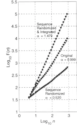
FIG. 1. Correlation properties of heartbeat interval time series. Original experimental time series
(upper left);
sequence-randomized surrogate data set(middle left);
sequence-randomized and integrated data set(lower left).
Scaling coefficients of time series(right).
14 MEYER ET AL.
TABLE 1
Scaling Coefficient a of Non-stationary Heartbeat Interval Time Series
Subject
24 hr e p o c h 4 hr s u b e p o e h 4 hr s u b e p o c hday-time
night-time
# 1 0.94 -4- 0.06 0.85 5= 0.05 ** 0.83 + 0.04 **,~ # 2 0.99 + 0.04 0.94 5= 0.07 ** 0.88 4- 0.03 **,+ # 3 0.98 5= 0.06 0.95 4- 0.09 ~ 0.89 4- 0.06 **,~ # 4 0.93 + 0.09 0.95 5= 0.11 ~ 0.81 5= 0.06 **,++ # 5 0.94 + 0.06 0.98 5= 0.06 * 0.82 4- 0.06 **,++ # 6 1.04 5= 0.05 1.00 5= 0.05 ~ 0.91 4- 0.03 **,++ # 7 1.04 + 0.02 1.04 4- 0.07 o 0.89 5= 0.04 **'++ # 8 1.04 5= 0.03 0.97 4- 0.06 ** 0.88 4- 0.05 **'++ # 9 1.01 5= 0.03 0.95 5= 0.08 ~ 0.84 4- 0.05 **'++ Group mean 0.99 + 0.04 0.96 5= 0.05 0.86 5= 0.04 Sherpa 0.98 5= 0.03 0.95 5= 0.08 ~ 0.84 5= 0.04 **'++Notes: Values of individual subjects are means + SD of serial measurements averaged over time of the experimental protocol. Paired t-statistics ~ NS, * P < 0.05, ** P < 0.01, four-hour daytime/nighttime subepochs vs. twenty-four-hour epochs; + P < 0.05, ++ P < 0.01, four-hour daytime vs. four-hour nighttime subepochs.
Correlation Properties of Time Series
The scaling exponent is related to different correlation properties of the time series: 1) for white noise which is composed of a sequence of independent random variables, a = 0.5; 2) for Brownian noise (classical random walk) which results from the integration of white noise where the individual steps are r a n d o m and uncorrelated, a = 1.5;
3) persistent long-range correlations exist for 0.5 < a < 1.0; and 4.) for
llf
noise whichrepresents the boundary between stationarity ( a < 1.0) and non-stationarity ( a > 1.0), a = 1.0. The finding of long-range correlations is indicative of self-similarity, scale-invariance, and a fractal pattern. Long-range correlations indicate that, on average, the fluctuations on one time scale are self-similar to those on other time scales.
A typical example of a non-stationary heartbeat interval time series is shown in Fig-
ure 1. The original time series derived from forty minute continuous E C G recording
(upper
left)
comprises three subepochs: 1) resting conditions, 2) square-wave cyclic exercise (50 W) indicated by an almost instantaneous decrease of heartbeat interval durations (increaseFRACTAL DYNAMICS OF HEART RATE AT ALTITUDE 15
integrated and detrended original time series yields a straight line with slope o~ - 1.0. Thus, the heartbeat interval fluctuations scale as F(n) ~ n l'~ indicating persistent non-trivial long-range correlations that are not the consequence of summation over random variables or artifacts of non-stationarity due to different levels of physical activities. The sequential ordering in the original time series may be eliminated by constructing a sequence-random- ized surrogate data set (middle left) with identical heartbeat interval distribution (i.e., same mean, SD, and higher moments) which demonstrates uncorrelated white noise (o~ - 0.5). Integration of the sequence-randomized surrogate set yields Brownian noise (lower left) with ~ approaching 1.5. If 0.5 < t~ < 1.0, the time series is correlated in time such that longer (shorter) heartbeat intervals are likely to be close to each other. If 1.0 < tx < 1.5, the time series is also correlated but the heartbeat interval sequence is more likely to alternate between long and short intervals ("anti-correlation"). Both the white noise and its integral, Brownian noise, are examples of true random processes with no (or trivial) dependency on their past history. The heartbeat interval time series produces a contour reminiscent of irregular "landscapes." The moderately rough landscape of llf fluctuations (o~ ~ 1.0) may be interpreted as a "compromise" between the very rough landscape of white noise (o~ - 0.5) and the very smooth landscape of Brownian noise (o~ ~ 1.5).
Experimental and Simulated Time Series
The DFA analysis was applied to the experimental heartbeat interval series of the full- length twenty-four-hour epochs. Typically, the data length ranged from 90,000 to 135,000 data points as a result of varying daily activities (trekking during ascent and laboratory work during sojourn at high altitude). A total of 150 twenty-four-hour ambulatory Holter recordings was analyzed. In addition, four hour subsets from 1:00 A.M. (P.M.) through 5:00 A.M. (P.M.) were selected from the original time series to determine the scaling proper- ties of nighttime and daytime subepochs that were twelve hours apart and differed in the subject's physical activity. The data length of these segments was 13,000 to 17,000 data points. Furthermore, the data were analyzed for consecutive one hour segments (number of points ranging from 3,000 to 10,000) and the results were properly aligned with respect to time allowing for the fact that the ECG recorders were started at different times of the day. The data length of the steady state short-term recordings in supine or sitting position was about 1,200 points.
In order to assess the effects of data length and of noise added to the signal on the accuracy and precision of estimates of the scaling coefficient o~, genuine time series with known correlation coefficients were generated with number of points ranging from N = 1024 (21~ to N = 131072 (217) and with o~ ranging from 0.5 to 1.5 (Keshner, 1982; Voss, 1988). Ten realizations were generated for each N and o~. For the noise analysis, Gaussian random noise was added to the genuine series with levels ranging from 5 percent to 500 percent of the standard deviation of the original signal. For statistical comparison, fitting of the scaling exponent o~ was restricted to a least-squares fit of log F(n) vs. log n for 16 < n < NI2, thus eliminating very large asymptotic time scales. For f'mite-length data sets the error of F(n) has been demonstrated to increase with n and scaling exponents calculated over a larger range of n have less accuracy (Peng et al., 1993a).
16 MEYER ET AL. 1400 ~" 1200 u~ E 1000 800 P a: 400 200 4 6 8 10 Number of Heartbeats ,,4 X 1 U 6 ...5 v 2 A 6 I I E 5 ---~, - - - v ~ 4 .---~--- i
g,a
"--O ..d / 13. 2 - 2 4 6 8 10Number of Data Points X 1 ^4
U i i i i i I I I i i I I i I I I i i I I i i i i i i I i i 1 i i " - - ~ . . . I - - - ' T - - - i I i I ,/': ', .~ubjeq't #7 / I 1 I I i 0 1 0 1 2 3 4 5 L ~ l o n I I I i i i i L - - _1 . . . i i i i
i--
Z
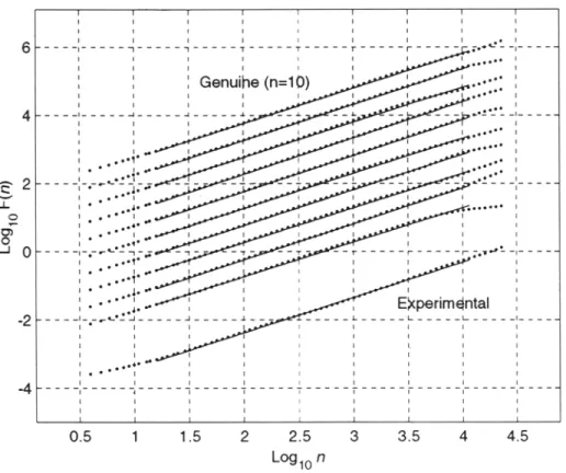
t i i i i i -7---,---~ . . . . i t I i i t I I I I 1 2 3 4 5 L ~ l o nFIG. 2. Detrended fluctuation analysis of twenty-four-hour heartbeat interval time series (upper) and genuine long-range power-law correlated fractal time series (lower). Scaling coefficients of time series (right).
Results
Experimental Time Series
Figure 2 (upper) shows the DFA analysis of a representative twenty-four-hour heartbeat interval time series (N = 102652 points) demonstrating power-law scaling over more than three decades with (x ~ 1, i.e., llf noise. For comparison, a genuine stationary sequence (same data length, mean, and dynamic range) with (z = 1.0 was generated (Figure 2,
lower). Visual comparison of the fluctuations of the experimental and genuine time series
remains ambiguous; nevertheless, the DFA analysis reveals that the correlation properties of the two series are close to identical.
Figure 3 shows the log F(n) vs. log n plots of serial twenty-four hour heartbeat interval time series from an individual subject (#7) during sojourn at high altitude. The DFA analysis demonstrates that the ~t exponents (slopes of the regression lines for 16 < n
< NI2) were close to 1.0 (overall mean + SD, 1.04 5: 0.2, range 0.99 to 1.07) and were
unaffected by the subject's exposure to a hypobaric (hypoxic) environment.
The results for the daytime and nighttime four hour subepochs in the same subject are summarized in Figure 4. Although not readily apparent upon visual inspection, the regres- sion slopes of the daytime four hour subsets (overall mean 5: SD, 1.04 5: 0.07, range 0.94 to
14 12 10 8 LL 0 6 I I I I (
FRACTAL DYNAMICS OF HEART RATE AT ALTITUDE 17
0 1 2 3 4 5
L ~ l o n
FIG. 3. Plot of log F(n) vs. log n (see description of DFA analysis) of twenty-four-hour heartbeat interval
time series of a subject sojourning at high altitude. The regression slopes for 16 <_ n <_ N/2 are shown by solid
lines. The plots are shifted vertically for the purpose of display.
1.10) were statistically indistinguishable from those of the full-length twenty-four-hour series. In contrast, the nighttime four-hour subsets (overall mean + SD, 0.89 + 0.04, range 0.84 to 0.95) were significantly lower (P < 0.01, paired t-statistics) compared to the daytime or full-length data series. These findings would suggest an apparent inconsistency of the DFA analysis which may be resolved by evidence that the twenty-four-hour time
series exhibits composite rather than unique fractal properties ( s e e D i s c u s s i o n ) . However,
of relevance here is the observation that both daytime and nighttime sequences do not show any systematic changes in response to high altitude.
Comprehensive results of the DFA analysis of serial twenty-four-hour heartbeat interval time series and its four-hour subsets of another subject (#8) along with the altitude profile and locations, covering sea level, ascent, sojourn at 5,050 m for thirty-four days, and return from altitude, are shown in Figure 5. The scaling exponent of the twenty-four-hour epochs varies from about 0.99 to 1.08 but is unaffected by the subject being exposed to hypoxia. No differences were apparent when the data from the initial stages of exposure to hypoxia were compared with those of the later stages. The overall mean value + SD of o~ (1.04 + 0.03) was statistically not different from 1.0, suggesting that heart rate fluctuations exhib-
ited l l f dynamics. The overall mean values + SD of the four-hour subepochs were 0.97 +
18 win'ore e'r AL. 12 10 8 12 Id. 0 6 10 4 4 2 2 0 0 I 2 3 4 I 2 3 4 L ~ 1 o n L ~ 1 o n
Fla. 4. Plot of log F(n) vs. log n of four-hour daytime (left) and four-hour nighttime (right) subepochs of twenty-four-hour heartbeat interval time series of a subject (same as Figure 3) sojourning at high altitude. The regression slopes for 16 < n < N I 2 are shown by solid lines. The plots are shifted vertically for the purpose of
display.
No systematic directional changes of a with exposure to hypoxia were observed in any of the nine subjects. The group mean average + SD was 0.99 + 0.04 (range 0.93 to 1.04) for the Caucasian subjects and was statistically not different from 0.98 + 0.03 calculated for acclimatized Sherpa natives (Table 1). The group mean day-night difference of oc of the four-hour subepochs was 0.10 + 0.05.
The lack of evidence of any effects of hypoxia on heartbeat interval dynamics in terms of potential readjustments during the early phase or acclimatization in the late phase of sojourn at high altitude is supported by the results compiled in Table 2 for the five subjects who were monitored simultaneously. The data base consists of six data sets each for the early and late phase, respectively. In the early phase, the subjects were monitored continu- ously for six days (separated by ten minute breaks) whereas in the late phase the record- ings were performed over a period of sixteen days (separated by forty-eight-hour inter- vals). There were no significant differences of the scaling coefficients in any of the five subjects (paired t-statistics), no matter whether the early vs. late comparison was based on the full-length twenty-four-hour epochs or four-hour day/night subepochs. However, the four-hour nighttime oc values were consistently lower than those of the four-hour daytime subepochs or the twenty-four-hour full-length epochs.
F R A C T A L D Y N A M I C S OF H E A R T R A T E A T A L T I T U D E 19 r- E
$
- r 120 110 100 90 80 70 60 50 40 1.2 1.1 v v 0.9 v 0.8 o~
0.7~
0.6 0.5 0.4 T r T 1 r T (386"/m)- 0 Namche E (3440m) Lukla (285 Pakding (2 -20 -10 Pyramid Laboratory (5050m) ro 9 9 ,.,Io . . . Z I - - " -9
9 9 Q _ _ _ _ _ o o o 0 0 | x)••
"~ ~ 9 Q I 9 . . . . 24 hr epoch o - - - 4 h r s u b e p o c h - d a y I, * - - 4 hr subepoch - nighl X X ~ ~ x x x x x x x x x Subject #8 0 10 20 30 40 50 DaysFio. 5. Scaling coefficients of twenty-four-hour, four-hour daytime, and four-hour nighttime heartbeat inter- val lime series of a subject during acclimatization to high altitude (5,050 m). The locations and altitudes of the measurements are indicated. The arrival at the Pyramid Laboratory is arbitrarily assigned as day 0. Resting heart rate was calculated from four-hour nighttime subepochs. Horizontal lines are means.
There is a limit to the ranges over which biological signals can be self-similar and time series cannot be arbitrarily short or long. The scaling coefficient 0~ was calculated for the concatenated heartbeat interval time series (48 to 144 hours) of the five subjects who were monitored simultaneously during ascent to high altitude. For segments of 48, 72, 96, 120, and 144 hours, respectively, the log F(n) vs. log n plots showed a progressive upward curvilinearity and o~ increased from about 1.0 (24 hour) to about 1.1 (144 hour) suggesting that the human heart rate fluctuations were self-similar over twenty-four hours but would not reach down to larger scales.
The results of the DFA analysis for one hour segments of the original time series are presented in Figure 6. All data in a given subject were averaged over the indexed hours of the day after proper alignment. The mean values + SD of the nine subjects for the scaling coefficient 0~ from 1:00 P.M. through 12:00 A.M. are displayed. The results are presented here just to indicate that all subjects had lower scaling coefficients during the night. However, it is important to emphasize that the data of Figure 6 could be potentially
misleading. The data wouM not reflect the actual pattern of change of 0~ throughout the
twenty-four hour period because the DFA analysis is based on scaling, i.e., estimates of the variance of the series at each of different levels of resolution (not time). Similarly, the data should neither be interpreted to suggest or imply that the scaling coefficient of the heart-
20 MEYER El" AL. .1 , , , , , , , , , , , , , , , , , , , , , , , 1 . 0 5
. •
0 . 9 5 C 3 8 0 . 9 ~ 0 . 8 5 0 . 8 0 . 7 5 9 ~ " . I fI
•
j _L 07, I I 1 I I 1 I t l I I I I I I I I i I I I I I i 1 3 1 4 1 5 1 6 1 7 1 8 1 9 2 0 2 1 2 2 2 3 2 4 1 2 3 4 5 6 7 8 9 1 0 1 1 1 2 H o u r o f t h e D a yFlG. 6. Scaling coefficients of one-hour subepochs of twenty-four-hour heartbeat interval time series. Mean values + SD of nine subjects. See text for details.
boat series was changing continually nor that a was changing on a hourly time scale. The results of the steady state short-term (twenty minutes) heartbeat interval series in supine and sitting posture are shown in Table 3. Again, these measurements did not reveal any effects from acute or chronic exposure to hypoxia. The group mean averages + SD
(0.95 + 0.05, supine; 0.95 + 0.07, sitting; ratio 1.00 + 0.16) were not different and were
close to the values of the full-length twenty-four hour epochs or four hour day-time subopochs (Table 1). These findings suggest that non-stationarity due to unsteady physi- ological conditions was unlikely to account for the fluctuations of the non-stationary twenty-four-hour time series and their ensuing scaling properties.
Genuine Fractal Time Series with Known Correlation Properties
Artificial stationary fractal time series with known a from 0.5 to 1.5 and lengths N = 131072 (217) points were generated to assess the accuracy (defined by the SD of the estimate) and precision (defined as absence of bias) of the DFA analysis. Ten realizations were obtained for each a and N. Shorter series from N = 1024 (2 l~ to N = 65536 (2 t6) were selected as part of the original series.
Figure 7 shows the results (means + SD for 10 realizations each) of estimation of the scaling coefficients for time series with N = 217 points for a ranging from 0.5 to 1.5. The absolute SD of the a estimates is about 0.0065. Hence, the accuracy of the estimates is
FRACTAL DYNAMICS OF HEART RATE AT ALTITUDE 21
TABLE 2
Scaling Coefficient a of Heartbeat Interval Time Series during the Early and Late Phase of Acclimatization to High Altitude
Subject
E a r l y P ho~-_~.e(is5o- 5o5o m)
day -6 - day 0 Late P h a s e (5050 , , ) day 18 - day 34Scaling Coe~cient (a) - PJ hr epochs # 2 1.00 4- 0.05 0.98 -4- 0.03
# 3 1.00 4- 0.05 0.98 4- 0.07
~:4 1.03 4- 0.04 0.98 4- 0.01
# 7 1.04 4- 0.03 1.04 -4- 0.02 # 8 1.05 4- 0.02 1.03 4- 0.02
Scaling Coe~cient (a) - ~ hr subepochs (day- time) # 2 0.94 4- 0.04 0.91 -t- 0.05
# 3 0.96 • 0.13 0.95 :t: 0.06 # 4 1.00 • 0.05 1.00 =t= 0.06
# 7 1.03 • 0.08 1.04 • 0.06
# 8 0.97 i 0.05 0.97 4- 0.04
Heart Rate (1/rnin) - ~ hr subepochs (night -
time)
# 2 62.9 4- 5.0 64.1 4- 7.2
# 3 58.3 4- 4.3 60.5 4- 4.3 # 4 60.0 -4- 2.9 58.6 4- 3.9 # 7 56.5 4- 2.9 56.9 4- 3.0 # 8 52.1 -4- 1.9 49.8 4- 2.6
2 2 MEYER ET AL.
T A B L E 2 (Continued)
Scaling Coefficient ( a ) - 4 hr subepochs (ni#ht - time) # 2 0.89 4- 0.03 0.88 • 0.03
# 3 0.87 + 0.06 0.87 • 0.05 # 4 0.83 + 0.06 0.79 • 0.05 # 7 0.89 4- 0.04 0.89 4- 0.04 # 8 0.88 • 0.04 0.87 4- 0.05
Notes: Values of individual subjects are means _+ SD of six consecutive measurements during the early phase (separated by ten-minute breaks) and six measurements during the late phase (separated by forty-eight-hour intervals) of acclimatization. Paired t-statistics for individual subjects do not reveal significant differences between early and late measurements. Day "0" is arbitrarily assigned to arrival at the Pyramid Laboratory (5,050 m). See Experimental Protocol and Fig. 5.
F I 1 I I i I ] I F I I I t i i I i t i i 1.5 . . . I t t t t i I t I I 4 I t I I I t I t I I r I _ 1 . 4 _ . . . . 9 . . . - - - - , . . . , . . . . ~ . . . ~ . . . - - - - ~ . . . . . * - / - - , - - - I t t ) i t t ) ~ ) I I t I t i I I I / I I I I t I I i I I is i I i 1 . 3 . . . . r . . . . r . . . . , . . . , . . . . n . . . . r . . . . r . . . . , . . . . = - - - ~ . . . . r . . . . I I i i t I t I i I t t l I I I I I I s t t t I I I I I , t 14 J t I I 1 . 2 . . . . T . . . . r . . . . , . . . , . . . . ~ . . . . T . . . . ' - - - . - - - , . . . . ; . . . . 7 - - - I I I I I t t / I I I l I i i I i I i J I I 1 ~ 1 . 1 . . . I I I I ~ . . . t ; ~ " . . . I I I t i t I i i , / ~ i i i i i . . . . + . . . . I-- . . . . t . . . I . . . . .-I . . . . . . . . t I t I t / 4 I t ~ I I I I I I I s I I I I I I . . . . T . . . . l- . . . . I . . . I . . . Z . . . . f- . . . . I . . . . "3 . . . . 7 . . . . I--- L I I I ~ ] I I I I I I I I I I ~ I ' I I I I t I i i ~ i i I t i I t 0 , 8 . . . . T . . . . F . . . . I . . . . . ---~1 . . . . ~" . . . . I . . . t . . . I . . . . ~ . . . . /--- I I I ~ I I i I I I I I I I I / I i , I I I I i %d # ~ " ~ 1 . 7 . . . . .L . . . . L _ _ _ " . . . . I . . . . / . . . . . L _ _ _ I . . . . I . . . . J . . . . .l . . . . J- . . . . t I I I i I I I I I I I I F j. t I I I i I I ww ~ q '- I I 0 . 6 . . . I ~ r I I I t I I I I I ~ ~ I t I I r I I I I I . . . . t 3 ~ I I I ~ I , I I I I A I I I L I L I I I 0 . 5 0 . 6 0 . 7 0 . 8 0 . 9 1 . 1 1 . 2 1 . 3 1 . 4 1 . 5 C~ predicted
Fro. 7. Estimation of the scaling coefficient a (ordinate) for genuine stationary fractal time series with
known correlation properties (abscissa). The results +_ SD are shown for ten realizations at each ct for et = 0.5 to tt = 1.5 and data length of 131072 (217) points. Dotted line is line of identity.
FRACTAL DYNAMICS OF HEART RATE AT ALTITUDE 23 1.5 1.4 , . , 1 . 3 E 9 -r 1.1 o 0.9 m r 0.8 ~0 0.7 0.6 0.5 i i ) i i i I f
iiiiii !
. . .
. . . " . . . ' . . . .
. . .
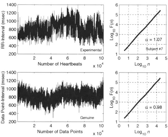
~ - . . . t . . . I . . . - - . . . . . . 6 5 ~ ~ - ~ - ~ - f . . . ~ . . . . - ~ - . . . . . . ~ . . . ~ - . . . ~ . . . ~: . . . ~ . . . .= . . . . ~ . . . . . . i . . . ~- . . . . - z - - ~ . . . I I . . . t - . . . 9 . . . ~ - . . . ~: . . . ~ . . . . . . . . . ~ . . . I I I -:r . . . _~_ . . . : t - r - - . Z - . . . . - , I - - , I . . . ~ . . . - - - - ~ - _~_ I I I I . . . t - ~ - - ~ " - - - ~ - . . . ' T , w . . . . ~ . . . ~ . . . . . . . . . . . . . X _ ~ I . . . x . . . --- . . . I ] ) I ~ ) ) i ] 10 11 12 13 14 15 16 17 D a t a L e n g t h ( N = 2 x)FIG. 8. E s t i m a t i o n o f the scaling coefficient a [[t a (]] (ordinate) for g e n u i n e stationary fractal t i m e series
with k n o w n correlation properties ( a = 0.5 to 1.5, horizontal dotted lines). The results + SD are s h o w n f o r 10
realizations at each a for data lengths ranging from 1024 (2 l~ to 131072 (2 tT) points (abscissa).
about 0.4 percent, 0.6 percent, and 1.3 percent for a = 1.5, a -- 1.0 and a = 0.5, respec- tively. The resolution, Aa, defined as three times the SD, for time series of length N = 217 (corresponding to the length of the experimental twenty-four-hour heartbeat interval series) and a ~ 1.0 is about 0.02. However, there is a small systematic error or bias in the a
estimates as the slope of the ~estimated VS. I~predicte d relationship is slightly less than unity
(0.97). Thus, the estimates of a are lower by about 3 percent of the true value over the range between a = 0.5 to a = 1.5.
The results for artificial time series with a values from 0.5 to 1.5 and lengths N from 21~ to 217 are shown in Figure 8. The SD is larger for short series ( - 0.06 for N = 21~ and decreases as a power-law function of N (~ 0.01 for N = 217), but the bias is about constant at < 3 percent over the range of N = 21~ to N = 217. Scaling coefficients derived from shorter experimental data sets may, thus, be compared with those of longer series but the results from shorter series are slightly less reliable. The source of the small bias in the estimates o f a is unclear and may be circumstantial due to inaccuracies of the method of signal generation, the DFA analysis, or both. Notwithstanding, the directional systematic error of the DFA analysis when applied to experimental data is small and, for the present study, would not invalidate any of the conclusions drawn.
2 4 MEYER ET AL.
TABLE 3
Scaling Coefficient a of Short-term Steady State Heartbeat Interval Time Series
Subject Supine Sitting
# 1 0.87 4- 0.13 0.87 + 0.06 # 2 0.92 + 0.06 0.90 + 0.07 # 3 0.93 4- 0.06 0.89 4- 0.08 # 4 0.94 4- 0.18 1.04 4- 0.06 # 5 1.01 4- 0.12 0.94 4- 0.11 # 6 0.93 4- 0.07 0.93 4- 0.06 # 7 1.06 4- 0.09 1.06 4- 0.06 # 8 0.94 4- 0.18 0.93 4- 0.07 # 9 0.91 4- 0.09 0.98 4- 0.12 Group mean 0.95 + 0.05 0.95 4- 0.07 Sherpa 0.89 + 0.10 0.90 + 0.07
Notes: Values of individual subjects are means • SD of serial measurements averaged over time of the experimental protocol.
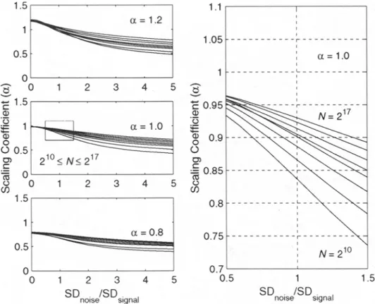
addition of Gaussian white noise ( a = 0.5) with zero mean and varied SDs from 5 percent to 500 percent of that of the original fractal time series. The results for a = 1.2, a = 1.0 and a = 0.8 for N = 2 l~ to N = 217 points and noise levels up to 500 percent are shown in Fig-
ure 9 (left). A window centered around SDnoisJSDsigna I = 1.0 (the added white noise has the same SD as the original signal) for a = 1.0 and N = 21~ to N = 217 points is displayed in
Figure 9 (right). As expected, added noise drives the effective correlation toward zero and
the estimate of a toward 0.5. The effects are less pronounced for series with larger N; the estimates of o~ remain closer to the true values at higher noise levels for N = 217 than for N = 2 l~ points. Fractal signals recorded with noise levels as large as 1.5 times the SD of the original signal appear to be safely distinguishable from true noise. In particular, for a = 1.0 and for large N the estimates of a are well determined from a single realization and are only moderately degraded even with the addition of 100 percent Gaussian noise.
The findings may be further generalized in that the estimation of a from a time series that consists of a combination of two fractal signals is biased toward that of the signal with
FRACTAL DYNAMICS OF HEART RATE AT ALTITUDE 25
1
.
5
~
1
= "
1.1
0.5
0
~"
0
1
2
3
4
5
0 0.5
0
I
oO 0
1
2
3
4
5 09
1"i . . .
1
0.8
0 5 ~
0.75
"C
. . . .
i
0.7
1 . 0 5 . . . oc= 1.0 . . . I I 1 2 3 4 5 ).5 1 1.5 SDnois/SDsigna ISDnoisJSDsignal
FiG. 9. Effect of noise on estimation of the scaling coefficient ct. Mean values of estimates of ct for ten genuine fractal time series with added Gaussian white noise (ordinate). The SD of the added noise is given as the ratio relative to the SD of the genuine fractal series (abscissa). The data are displayed for ~ = 1.2, ct = 1.0, ct = 0.8 and data lengths from 2/7 to 21~ points (upper to lower curves). A magnifying window indicated by rectangle (left, middle) is displayed for better viewing (fig/u).
the higher scaling coefficient. However, long-range correlations with power-law character- istics cannot trivially be generated from fractal signals modulated by multiple time scales. For example, the superposition of white ((~ = 0.5) and brown (ix = 1.5) noise would not produce long-range correlations or l / f dynamics ((~ = 1.0) no matter how the amplitudes of those components are varied.
However, a source of weakness becomes evident from the log F(n) vs. log n relation- ships (Figure 10). The effects of Gaussian noise (5 percent to 500 percent) for o~ = 1.0 and N = 217 points (left) or N = 2 l~ points (right) are displayed. Increasing levels of noise lead to distortion of the normally (for genuine stationary single-component fractal time series) straight-line log F(n) vs. log n relationships with the initial slope for small n differing from the asymptotic final slope for large n (cross-over). Thus, the estimated scaling coefficient, in the presence of noise, would strongly depend on the range n over which the slope is calculated.
The noise inherent in the experimental heartbeat interval time series is a priori un- known. In order to exclude the possibility that fluctuations due to instrumentation and measurement errors could account for the correlation properties inferred from the scaling
26 METER ~ AL. 10 .I . I . . I . I I I I 4 - t I I I I 8 6 4 4 "E" v v LL LL ~ R2 o o -- 2 _,,I 0 -2 0 -2 -4 -4 1 2 3 4 5 1 2 3 L ~ l o n L ~ l o n
Fro. 10. Effect of noise on estimation of the scaling coefficient ct. Plot of log F(n) vs. log n for t~ = 1.0 and
N = 217 data points
(left)
and N = 2 ~~ data points(right).
See text for details.analysis, the ECG was recorded from an analog ECG signal generator that could generate ECG waveforms at different frequencies with or without superimposed modulations (e.g., sinus arrhythmia). For the range of heart rate between 40/minute to 200/minute corre- sponding to interval lengths of 1,500 msec and 300 msec, respectively, the coefficient of variation was 0.4 percent. Under real-life conditions the error may be larger due to noise incurred from skeletal muscle contractions and the floating nature of the ECG signal but would not be expected to exceed 5 percent. Assuming that the fraction of the noise in the signal was less in the four-hour nighttime heartbeat interval series compared with the four- hour daytime series because the subjects were physically inactive (sleeping) and the heart rates were generally low ( - 60/minute), the difference between the group mean values
(0.86 vs. 0.96,
cfi
Table 1) is likely to be due to reasons other than differences of the levelsof noise in the series (because o~ is biased toward lower rather than higher values in the
presence of noise). Similarly, cross-over of slopes in the log F(n) vs. log n plots
(cfi
Figure10) was typically not observed for the experimental data series
(cfi
Figures 3 and 4).In summary, the DFA analysis is quite robust in three points: 1) proper estimates of the correlation properties of the time series may be obtained from series as short as 1,024 points; 2) the bias in the estimated scaling coefficient a is small (< 3 percent); and 3) the method is not highly sensitive to noise.
FRACTAL DYNAMICS OF HEART RATE AT ALTITUDE 27
Aside
The ECG recordings, by clinical evaluation, were free from pathologic changes in all subjects. Specifically, the abundance of ectopic beats or changes of the ST-segment were in the normal range. Resting heart rate during sleep obtained from the four hour nighttime heartbeat interval series was 61 + 8 beats/minute (group mean + SD). Resting nighttime heart rate was unchanged by hypoxia as reflected by the comparison of the early and late phase data (Table 2,
bottom).
Most of the evidence from the literature suggests that day- time resting heart rate is increased during the early phase but levels off during the later stages of acclimatization to high altitude. The initial increase could be associated with mild symptoms of acute mountain sickness from an improper state of acclimatization (observed in about 75 percent of subjects sojourning at high altitude). It would seem that our data demonstrating absence of any effects of hypoxia on resting heart rate are perfectly in line with the very early heart rate measurements by simple pulse counting (before rising in the morning, at absolute rest, and on an empty stomach) obtained in members of the German expeditions to Nanga Parbat in 1937/38 and the brief review by Luft (1988) on these studies is worth reading.Arterialized (ear lobe) blood 02 saturation (So2 [percent] mean + SD of six subjects) was 81 + 6, 82 + 5, 83 + 5 after 1, 3, 5 weeks sojourn at 5,050 m altitude, respectively.
Discussion
To our best knowledge, the present study is the first dynamical analysis of heart rate fluctuations in normal subjects during long-term (> fourteen days) exposure to high (> 5,000 m) altitude hypoxia.
The analysis of scaling properties of long-term twenty-four-hour heartbeat interval time series has revealed three important findings: 1) The long-term fluctuations of heart rate exhibit long-range, scale-invariant, power-law characteristics (scaling exponent r - 1, i.e.,
llf
noise) reminiscent of dynamical systems far away from equilibrium (Bak and Creutz, 1994; Stanley, 1971). 2) The intrinsic dynamics of the heartbeat interval fluctuations, i.e., l/f behavior, is essentially unaffected by the physiologic challenge of chronic exposure to hypoxia. The results are consistent with our hypothesis that the intrinsic mechanisms generating fractal I/f dynamics of heartbeat fluctuations are unaffected by chronic hypoxia, i.e., the intrinsic heartbeat dynamics do not undergo early readjustment or late acclimatiza- tion. 3) The analysis of the four-hour daytime and four-hour nighttime subepochs selected as subsets of the full-length twenty-four-hour time series has revealed an apparent discrep- ancy in that the scaling properties of the heartbeat interval series during nighttime episodes were lower (r = 0.86 + 0.04) compared to the daytime episodes (r = 0.96 _+ 0.05) or the twenty-four-hour periods (r = 0.99 + 0.04). These findings suggest that the fractal charac- teristics of heart rate in the course of a twenty-four-hour period of observation were evolving with time and became local, i.e., the signal is what is generally referred to as amultifractal.
However, the multicomponent composite fractal nature of the time series would remain unnoticed by the DFA analysis when applied to the full-length twenty-four- hour data base.The effects of high altitude hypoxia on the variability of heart rate has been addressed by Hughson et al. (1994). A coarse-graining spectral analysis technique (Yamamoto and Hughson, 1991; 1993) was employed to separate the harmonic and non-harmonic, i.e., fractal, components of short-term (10 minutes) heartbeat interval time series. While the
2 8 MEYER Ft" At..
analysis of the harmonic components demonstrated an increase of the sympathetic activity associated with a decrease of the parasympathetic activity soon after exposure to moderate altitude (4,300 m) there was a tendency to return to sea level values after twelve days sojourn at that altitude. The fractal component was decreased in response to altitude exposure compared to sea level controls but the significance of this finding was not addressed. Later on, by incorporation of more data, the authors felt that the fractal compo- nent had remained unchanged (personal communication).
Non-Stationarity and Fractal Dynamics
Conceptually, physiological time series such as heartbeat interval time series under free-running conditions may be visualized as "badly behaved" data originating from non-stationarities driven by uncorrelated extrinsic factors and/or from the intrinsic non-linear correlated dynamics of a fractal process. Hence, any analysis of heartbeat inter- val time series is confronted with the problem of distinguishing a stationary fractal time series from a non-stationary process.
Formally, the signal generated by a fractal process is non-stationary, i.e., it varies all over as a result of its "built-in" long-range power-law properties and its moments depend on time. A fractal generating mechanism with fixed components can generate a time series with moments that vary in time. A self-similar fractal process typically produces a time series with long-range correlations of the fluctuations that display the kind of "drift-like" appearance at all time scales. The statistical properties of a fractal process axe character- ized by an infinite mean or infinite variance and the mean of a measured property changes with the amount of data analyzed and would not converge to a well defined value. Hence, non-stationarity only indicates that the moments are not defined but would not imply that the process that generated the data was changing in time. The situation is further compli- cated by the fact that a fractal process may not be completely described by a unique scaling coefficient (or single fractal dimension) because it may present a composite of fractals with varying scaling properties (or different fractal dimensions).
On the other hand, the intrinsic dynamics of a complex non-linear system may be biased by extrinsic sources, i.e., non-steady state physiological or environmental conditions, that could give rise to highly non-stationary behavior. Although these strain-related variations may be physiologically important, their correlation properties would be expected to be different (i.e., related to the stimulus) from the long-range correlations ("memory") gener- ated by a dynamical system.
The twenty-four-hour heartbeat time series of the present study were highly non-station- ary with heart rates ranging from 40/minute (nighttime supine resting conditions) to about 200/minute (daytime physical activity up to exhaustion). A key issue of the detrended fluctuation analysis is that the extrinsic fluctuations from uncorrelated stimuli can be interpreted as "trends" and decomposed from the intrinsic dynamics of the system itself. The principle of calculating a measure of dispersion (F(n)) as function of window size (n) consequent upon subtracting the local trend in each window facilitates the detection of intrinsic long-range correlations embedded in a non-stationary time series.
In Figure 11 the log F(n) vs. log n plots are shown for an experimental time series (t~ = 1.032) and ten realizations of a genuine stationary fractal process with the same scaling exponent. The regression slopes (16 < n < NI2) of the genuine time series (mean 5: SD, 1.036 + 0.018, range 1.009 to 1.061) were not statistically different (t-test of regression slopes) from the experimental series suggesting that the experimental series was in fact
FRACTAL DYNAMICS OF HEART RATE AT ALTITUDE 29 i I I : ; ~ I ; I I I i I I i q I I I i I I I o" I I I I t I I t ,io I , , n u | h e ( n = l O ) - . . . ' : . , I I I I I I Iee l= I I I I I I I I I I eee ee" I ' . , - ~ ~ ~ __1...'~ ~ ...,~"" , ~ " o~ .. ....--- ~ _ r _ ~ . ~ J , ~ ~ j..o-" ~149 i ~ 2 , . - . ~ . . , , - - - ;,.r.,.- - - t , ; ' - - Z , . ~ " - ' - . P ~ - -7.~, " r r - ; . ; ~ ~ 9176 ~ ~ ~ . ~ , - ' ~ . ~ . , ~ ,,.,~-" , * ., 9 -" ~ ~ _~,~J"~ / ~ , o . . . . . . . , . . . , ~ ~176 . . , . i - ~ ...~.~.r , , . . . ~ , , . o . - I ~ ~ , , _ _ ~ , ~ , , I 9 ~ ~ ~ m ~ e ' " I I I / I I I ' . " " " ' / ' ~ ' I:::~r~ i a t I r i , . . , . . . ~ _ , . ~ . r m . , n . a , - 2 ,. ,, ~ , . . . ~ . . . ,, oQ4~ ~ I I 9 *~176 I I I I I I "4 . . . ~ . . . i . . . ~ . . . I t i I I I 0 . 5 1 1 . 5 2 2 . 5 3 3 . 5 4 4 . 5 LOglo n
FIG. l 1. Plot o f log F(n) vs. log n for a typical experimental twenty-four-hour heartbeat interval time series and ten realizations o f a genuine fractal times series with the same length and scaling coefficient. The regres- sion slopes for 16 <- n < N I 2 are shown by solid lines. The plots are shifted vertically for the purpose of display.
generated by a stationary fractal process with l / f dynamics (strictly, this is strong evidence, not proof).
Unlike conventional methods (e.g., power spectrum analysis and Hurst analysis) that presume stationarity of the data stream, the DFA technique does not rely on this assump- tion. Indeed, the persistence of long-range correlations after detrending would be indica- tive of a genuinely self-similar process. In order to rule out the possibility that the fluctua- tions in the experimental time series and their long-range correlations were simply a trivial consequence of extrinsic non-stationarities, the data series were detrended prior to apply- ing the DFA analysis. A typical example is shown in Figure 12 (left). Detrending was performed by fitting the data by polynomials of order 1 to 5 and then by subtracting the fitted curve from the data. The procedure was performed at multiple time scales, i.e., the original time series was detrended for segments with N ranging from 210 to 217 data points. In the example of Figure 12 (left) the estimated scaling coefficient (x for the experimental time series (N = 131072 data points) prior to detrending was 1.04, and for segments varying from N = 216 to N = 2 ]0 points remained practically unchanged (range 0.99 to 1.05), but the SD of the estimates increased with shorter data sets (cf. Figure 8 and Results Section). The lower and higher order detrending is expected to remove much of the slow
3 0 MEYER ET AL. Experimental 1.5 no detrend'. 1 1 : - " - O.fi 1'5}I + .._.. ! t"- 0.5 + 1++ O ~ 1}1 z ]J J I J J ]
~os t
) I
~ I ] Ip~
d 1 z
.3,
0.5 t pol. deg. 1 1 I 1~L d~. 2
l ] I st 1.5 1 0.5 1.5 1 0.5 Unique Composite no detrend. 1.5 no detrend. 0.5IDol. deg. 1 1.5 I[ + IDO I. dog. 1
" " " " ~ " I 1 1 t 0.5
1-51
pot. d~. 2 0.5 1"5f, ~ pol. deg. 4 15 f 1 ,[ I 2 1 2 J" . z ] ] I I l 1 ,! 0.5 ' 0.51.5[ , i l z ,t ,1 t I .I . / pol. deg. 5 1"if
m [ i z ] ] l ] 1 r 0mS { . . . 01 10 11 12 13 14 15 16 17 1.5 ) IDol, de9. 2 0.5 / 1.5 f pol, deg. 3 0.5 L
13OI. deg. 4 1.5 f pol. deg. 4
0+5 '
pol. deg. + 1.+ [ pol. d~j+ S e ", ~- = ~ ~ 15 [
0 . ' ' ' ' ' ' ' '
10 11 12 13 14 15 16 17 10 11 12 13 14 15 16 17 Segment Length
(N =
2 x)Fzo. 12. Effects o f detrending o f experimental (left) and fractal time series with unique (middle) or compos-
ite (right) fractal properties. See text for details.
varying "drifting" in the time series but has almost no effect on the estimated scaling coefficient because the short-scale fluctuations would remain practically unchanged.
For comparison, the results of the detrending procedures are shown in Figure 12
(middle)
for a genuine stationary fractal time series with a unique scaling coefficient (e~ =0.99,
llf
noise). As expected, detrending has little effect on the scaling coefficient of a genuinely self-similar process. Detrending of a composite fractal time series is shown in Figure 12(right).
In the original time series (o~ = 0.99, Figure 12,middle)
the central segment of length N = 39322 data points (= 30 percent) was replaced by a subset with a = 0.79. Thus, the fractal time series was non-stationary by the scaling coefficient of the composite time series switching between e~ ~ 1.0 and a - 0.8. The scaling coefficient of the composite time series was 0.97 and, thus, was only about 2 percent smaller than that of the original stationary unique fractal time series. Of interest to note is that the scaling coefficient was practically unchanged upon detrending, but the SD of the estimates in- creased for shorter segments. The same behavior is observed for the experimental time series (Figure 12,left)
suggesting that the experimental time series had the characteristics of a composite rather than unique fractal process.By definition, a long-range correlated time series, irrespective of being generated by a composite or unique fractal process, consists of the "drift-like" or "trend-like" fluctuations
FRACTAL DYNAMICS OF HEART RATE AT ALTITUDE 31 1.05 r 1 to 0.95 0 o t- 0.9 o U) 0.85 0 ,---. 1,05 ~5 a~ 1 ._ a~ 0.95 0 r- 0.9 . h o 09 0.85 0 .... . . . R e p l a c e m e n t " ~ ~ 0 0 ~=o.9 ~ ' ~ , ~ { ~ \ ~ 7- e - - o _ ~,= o.8 ~ % . ~ O - - O a = 0.7 t " " . - ~ l J ~ T 0 0 a=o.6 \ ~ r , - ~ - - ~ Stem Spries N = 217 ~ = 1.0 , , - 20 40 60 80 100 R e l a t i v e L e n g t h of S e g m e n t a l R e p l a c e m e n t (%) t I I I . . . w . . . w .... I ~ ~ 0 0 ct = 0.9 i - " " O---O et= 0.8 ~ - O et = 0.7 O O or= 0.6 9 ~ ,,o ct = 0,5 Replacement a = 1 o0 20 40 60 80 R e l a t i v e Length of Segmental R e p l a c e m e n t (%) 00
Fro. 13. Estimation of scaling coefficient a for composite fractal time series. See text for details.
at all time scales that cannot be removed systematically. In contrast, if the long-range correlations were to disappear upon detrending (expected to be associated with a break-down of the scaling properties) then, most likely, it was only the presence of the trends that led to the "spurious" finding of the long-range correlations. The finding that the scaling coefficient of the experimental series remained unchanged even with higher order detrending is strong evidence that the long-range correlations were not an artifact of non-stationarity. Thus, the observed "drift" (Figure 2) is an indication of a fractal process and is the consequence of the "built-in" long-range power-law correlations. By the same reasoning, superposition of non-stationary external trends onto control time series with scale-invariant self-similar properties has been demonstrated to have almost no effect on the scaling properties of the series (Hausdorff et al., 1996; Peng et al., 1993a).
Composite Fractal Time Series and Scaling Properties
In the calculation of the scaling coefficient o~ by the DFA analysis, it is assumed implicitly that the process underlying the fluctuations inherent in the time series analyzed constitutes a single fractal process with unique scaling properties. The apparent discrep- ancy of the results of the experimental four hour daytime/nighttime time series (Table 1) suggests that the fractal properties of the time series were not constant in time but were
32 MEYF_~ ET AL.
changing and, thus, were locally different in the full-length twenty-four-hour series. In order to explore this possibility, composite fractal time series were generated by replacing segments of varied length N of a given time series with known 0c by segments of another time series with differing known or.
The results are shown in Figure 13. In the stem series (N = 217 points, o~ = 1.0), randomly selected segments of length N varied from 10 percent to 90 percent of the full length of the series were replaced with segments randomly selected from another series with ot varying from 0.9 to 0.5. Ten realizations were calculated for each combination of fractional segmental length and ct (for 100 realizations the results were the same). The segments were selected randomly in order to take into account that the experimental ECG recordings were started at different times of the day and hence the position of the nighttime episodes varied within the time series. It is seen that the scaling coefficient o~ calculated by the DFA analysis is pushed away from its original value when the fraction of the segmen- tal component is increased, finally approaching that of the series which is used for replace- ment (Figure 13,
upper).
An approximately mirror image is obtained when fractions of the stem series (N = 217 points) and varied ~ (0.9 to 0.5) are replaced by equivalent segments with ot = 1.0 (Figure 13,lower).
Interestingly, the effects are relatively small and even 90 percent replacement causes ot to decrease by about 15 percent only. Hence, for a composite fractal time series the component with higher ot strongly dominates the calculated scaling exponents and the effects are slightly smaller when the difference between the ot values is large. Assuming that the experimental subjects had been sleeping for 7.2 hours (30 percent of a twenty-four-hour epoch) and their heart rate scaling coefficient during the nighttime subepochs was ot = 0.8 and otherwise was 0~ = 1.0 during the remaining period, the effect is of the order of 2 percent only. These findings would resolve the conflict that the lower scaling coefficients calculated for the four-hour nighttime subepochs were not reflected in the calculations that were based on the full-length twenty-four-hour time series. On the other hand, these simulations add to the suggestive evidence that the experimental time series had a composite rather than unique structure, i.e., were multifractals. It is therefore appropriate that the scaling exponents calculated for the twenty-four-hour full-length se- ties, ot - 1.0, i.e., I/f dynamics, may be considered as "apparent" scaling coefficients.Tracking the composite nature of heart rate fluctuations (the composite feature of an experimental time series is generally a priori unknown) is facilitated by constructing
Amplitude-Adjusted Surrogate
data from the original time series (cf. Kaplan and Glass,1995; Theiler et al., 1992). Surrogate data has two important properties in that the process underlying its generation is both stationary and linear (absence of any dynamical non-linearities). The mean, variance and power spectrum of the surrogate data are identical to that of the original test data. Informal examples are presented in Figure 14. Two genuine fractal time series (~x = 1.0, o~ = 0.8; N = 217) were used and each split into segments of length N = 212 (4096), N = 213 (8192), N = 214 (16384), respectively. For each segment ten realizations of amplitude-adjusted surrogate data were calculated and the scaling coeffi- cient ~ calculated by the DFA-technique for the individual realizations of each segment
(Segment-by-Segment Surrogates).
Next, ten realizations of amplitude-adjusted surrogatedata were calculated for the full-length series (N = 217) and the surrogate data series were split into segments of N = 212, N = 213 and N - 214, respectively
(Surrogates Split into
Segments).
Again, o~ was calculated for the split surrogate segments. In Figure 14(upper)
the results are presented by plotting ~ for the surrogates split into segments


![FIG. 8. E s t i m a t i o n o f the scaling coefficient a [[t a (]] (ordinate) for g e n u i n e stationary fractal t i m e series with k n o w n correlation properties ( a = 0.5 to 1.5, horizontal dotted lines)](https://thumb-eu.123doks.com/thumbv2/123doknet/14877324.642760/15.729.104.628.137.566/scaling-coefficient-ordinate-stationary-fractal-correlation-properties-horizontal.webp)