Spiral FFAG lattice design tools

(1)

HAL Id: in2p3-00154218

http://hal.in2p3.fr/in2p3-00154218

Submitted on 13 Jun 2007

HAL is a multi-disciplinary open access

archive for the deposit and dissemination of sci-entific research documents, whether they are pub-lished or not. The documents may come from teaching and research institutions in France or abroad, or from public or private research centers.

L’archive ouverte pluridisciplinaire HAL, est destinée au dépôt et à la diffusion de documents scientifiques de niveau recherche, publiés ou non, émanant des établissements d’enseignement et de recherche français ou étrangers, des laboratoires publics ou privés.

J. Fourrier, F. Martinache, F. Méot, J. Pasternak

To cite this version:

J. Fourrier, F. Martinache, F. Méot, J. Pasternak. Spiral FFAG lattice design tools - Application to 6-D tracking. 2007, 19 p. �in2p3-00154218�

(2)

Application to 6-D tracking

J. Fourrier

†

_{, F. Martinache}

†

_{F. M´eot}

‡

_{, J. Pasternak}

† †_{CNRS IN2P3, LPSC, Grenoble}

‡_{CEA et IN2P3, LPSC, Grenoble}

Abstract

Ray-tracing based methods for 3-D modeling of magnetic field and particle motion in spiral scaling FFAG accelerators have been developed. They allow efficient simulation of particle motion in presence of the strong field

non-linearities proper to FFAG magnets, and of possible field overlapping in configurations of neighboring magnets, thus yielding a performing tool for spiral FFAG lattice design and optimizations, and for 6-D track-ing studies. It is applied for illustration to a principle design of a

200 MeV medical class proton FFAG now under study in the frame of the RACCAM hadrontherapy project.

(3)

In the context of these collaborations, and in particular that of the RACCAM FFAG project [9, 10], works have recently been undertaken concerning ray-tracing code developments regarding spiral FFAG lattice, in view of medical machine design in the short term, and possible application to muon rings for the scaling FFAG based neutrino factory, as well as high-power beams, in the longer term.

A good knowledge of FFAG accelerator parameters can only be drawn from stepwise ray-tracing in realistic field models. In particular this is the only method that allows computation of the dynamical acceptance of the ring. The developments presented here concern the implementation of such FFAG dedicated tools in the computer code Zgoubi [11, 12]. This has various outcomes, as offering means for fast optimization of magnet geometry and fields as constrained by accelerator design parameters ; providing correct computation of periodic motion, tunes, amplitude and momentum detunings, time of flight, etc. ; yielding precision tool for 6-D multiturn tracking, resonance and dynamic aperture studies. In addition, preliminary adjustments of magnet/field parameters can be performed thanks to the built-in fitting procedure, whereas optimizations based on 3-D magnet code calculations have the inconvenience of being slow and lacking flexibility in that matter.

The paper is organized as follows. Section 2 describes the main ingredients and methods in the mod-eling of spiral FFAG magnets. Section 3 shows an application to design issues, from determination of first order parameters to dynamic aperture scan. Section 4 discusses longitudinal dynamics and 6-D simula-tions.

2 A spiral magnet procedure

This Section describes the way the vertical field component Bz(r, θ) and derivatives at all position in

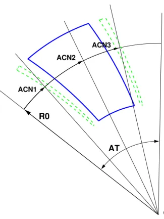
the median plane of a magnet composed of neighboring spiral sectors (Fig. 1) with possibly overlapping fields are calculated, thus allowing the calculation of the field vector and its derivatives, as involved in the ray-tracing numerical method [11].

The various magnetic sectors are positioned within an angular domain AT , in the cylindrical frame with origin O at the center of the ring, using a reference radius R0and positioning angles ACNi(Fig. 1).

The Bz(r, θ) calculation method is derived from an existing procedure regarding radial type FFAG

magnets, presented in an earlier works [12], and yields a new routine, referred to as “FFAG-SPI” in the following.

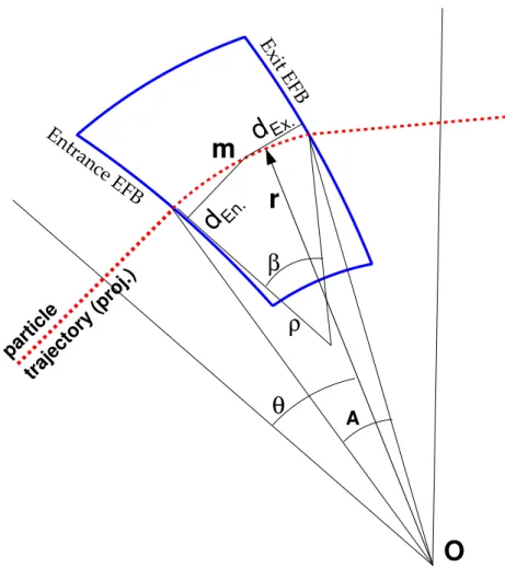
The main ingredients are as follows. The magnetic field in the median plane (z = 0) of a spiral sector, in cylindrical coordinates (r, θ) (Fig. 2), is written

Bz(r, θ) = Bz 0F(r, θ) R(r) (1)

wherein Bz 0 is a reference field taken at reference radius R0. The factor R(r) models the r dependence

of the field, and can be expressed under either form R(r) = µ r R0 ¶k(r) or R(r) = b0+ b1r − R0 R0 + b2µ r − R0 R0 ¶2 + ... (2)

with k(r) being the field index. Note that in the classical scaling FFAG optics k is in principle a constant, however in the present numerical approach it is allowed to be dependent of r : this permits designing possible compensation of the alteration of scaling properties under the effects of fringe field shape and extent, see below.

(5)

AT ACN1 ACN3 ACN2 R0 O

Figure 1:Definition of a spiral FFAG magnet, using the “FFAG-SPI“ procedure. Several sectors with overlapping fields (clamps, here) can be accounted for.

The magnet EFBs have a spiral geometry with equation r = R0eb(r)θ, with b(r) = 1/ tan ξ(r)

and ξ(r) the spiral angle. In principle again ξ is constant, however FFAG-SPI allows r-dependence, so to provide a mean for recovering scaling properties in case of perturbating effects as fringe fields, r-dependence of k, etc. The ensuing axial field form factor F(r, θ) (sometimes modelled in analytical approaches by 1 + f sin(N(θ − tan ξ ln(r/r0))), for a N sectors ring, with f the “flutter” [13]), gives

the spiral azimuthal dependence of the field, and in the present ray-tracing tools is modelled in the way detailed below.

Field fall-offs The field fall-off (Fig. 3) at a particular effective field boundary (EFB) is written [14,

p. 240]

FEFB(d) =

1

1 + exp[p(d)]) , p(d) = C0+ C1d/g + ... + C5(d/g)

5 ₍₃₎

wherein d is the distance to that EFB and depends on r and θ (dEn.and dEx.for respectively the entrance

and exit EFBs in Fig. 2), and the coefficient g is normally homogeneous to the gap and can be a function of r, see below. The distance d is computed by numerically solving for θ the equation [15]

(Xm− ebθR0cos(ω + θ)) (b ebθR0cos(ω + θ) − ebθR0sin(ω + θ)) + (4)

(Ym− ebθR0sin(ω + θ)) (ebθR0cos(ω + θ) + b ebθR0sin(ω + θ)) = 0

which tells that the normal to the spiral EFB at location θ contains the observation point, i.e. m = (Xm, Ym)(therein the angle ω is the EFB angular position in the reference frame). The numerical

co-efficients C0− C5are supposed to be known, for instance from prior matching with realistic fringe field

(6)

Ex.

d

En. Exit EFB trajectory (proj.) particle Entrance EFB

m

O

β

ρ

r

θ

_A

Figure 2: Ingredients entering in the computation of the mid-plane field Bz(r, θ)in a spiral sector magnet.

-.1 -.05 0.0 0.05 0.1 0.0 0.2 0.4 0.6 0.8 1.

F_EFB vs. d/g

(7)

Noteworthy, an adequate positioning of the EFB makes possible to satisfy (referring to the frame as defined in Fig. 3) Z 0 d=−∞F EFB(u) du = Z ∞ d=0(1 − F EFB(u)) du

which entails that varying g (as ensuing from r dependence, for instance, see Eq. 5) will not change the magnetic length, it will only change the fall-off steepness. This has the convenient consequence of allow-ing the simulation of various gap geometries as

g(r) = g0(R0/r)κ, κ ≈ k gap shaping (5)

g(r) = Cst (κ = 0) parallel gap

g(r) = g0r/R0 (κ = −1) linear gap

From a practical point of view, the first g(r) dependence simulates the case where the field law Bz(r) =

B_{z 0}(r/R0)kensues from the gap shape (so called “gap-shaping” method), whereas in the second and third

cases Bz(r)is supposed to be obtained from coil distributions in the gap. Note that the linear gap case

ensures r-invariant vertical tune, as addressed in Section 3.

Both entrance and exit EFBs have their own fringe field factors, FEn., FEx.. The form factor at particle position (r, θ) is thus written

F(r, θ) = FEn.(r, θ) × FEx.(r, θ) (6)

Full field at arbitrary position Now, accounting for n neighboring sectors (for instance, a main dipole

and field clamps as schemed in Fig. 1), the mid-plane field and derivatives are computed by addition of the contributions of the i = 1, n sectors taken separately, namely

Bz(r, θ) = X i=1,n Bz 0,iFi(r, θ) Ri(r) and ∂k+l_B_~ z(r, θ) ∂θk_∂rl = X i=1,n ∂k+l_B_~ z i(r, θ) ∂θk_∂rl (7)

Note that, in doing so it is not meant that linear field superposition actually applies, it is just meant to provide the possibility of obtaining a realistic field shape, that would for instance closely match (using adequate C0− C5sets of coefficients, Eq. 3) 3-D field distributions obtained from magnet codes or from

measurements. This procedure is illustrated in

(i) Fig. 4 that shows the field distribution in the median plane of a spiral magnet with field index k ≈ 4 and spiral angle ξ ≈ 50 degrees,

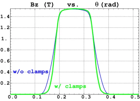
(ii) Fig. 5 that shows the field resulting from the superposition of a central dipole and of field clamps (simulated as powered thin magnets) as schemed in Fig. 1.

The 6-D field ~B(r, θ, z) and derivatives ∂k+l+m_B/∂r~ k_∂θl_∂zm _{at particle location are eventually}

deduced by z-extrapolation accounting for Maxwell equations [11, 12].

Calculation of the mid-plane derivatives (Eq. 7) can be performed using one or the other of the

fol-lowing methods, upon option,

(i) numerical interpolation from a “flying mesh”. In this case Bz(r, θ, Z = 0)is computed at the n ∗ n

nodes (n = 3 or 5 in practice) of a “flying” interpolation mesh centered on the actual (r, θ, z = 0) particle position projection (m in Fig. 2).

(ii) use of a 2-D mid-plane magnetic field map (Fig. 4) that encompasses the all magnet, computed before-hand using the procedure above.

In addition, a third method is under installation, fully based on analytical expressions of Bz(r, θ)and

derivatives ∂i+j_B

z(r, θ)/∂ri∂θj, as was done for the radial FFAG magnet [12].

The first method has the merit of allowing parameter optimization using the built-in fit procedure. The second one has the merit of faster tracking. Both feature excellent symplecticity - dependent upon

(8)

20 40 60 80 100 10 20 30 40 0 5 10 15 20 40 60 80 100

Figure 4:Spiral magnet field map as obtained from Eqs. 1-6.

0.0 0.1 0.2 0.3 0.4 0.5 0.2 0.4 0.6 0.8 1. 1.2 1.4

θ

Bz (T) vs. (rad)

w/ clamps

w/o clamps

Figure 5: Typical axial dependence Bz(r0, θ)(Eq. 7) of the mid-plane field, as observed at traversal of a spiral

(9)

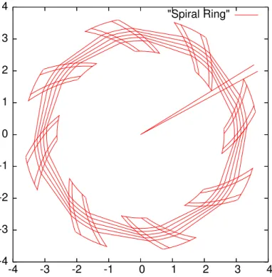
-4 -3 -2 -1 0 1 2 3 4 -4 -3 -2 -1 0 1 2 3 4 "Spiral Ring"

Figure 6:Spiral ring and a set of closed orbits taken between 0.6 T.m (17 MeV proton) and 2 T.m (180 MeV).

0.0 2.5 5.0 7.5 10.0 12.5 15.0 17.5 20.0 22.5 25.0 s (m)

δE/ p0c = 0.

Table name = TWISS

Linux version 8.23/06 10/02/07 21.48.14 0.0 1. 2. 3. 4. 5. 6. β (m ) 0.0 0.1 0.2 0.3 0.4 0.5 0.6 0.7 0.8 0.9 1.0 D x (m ) βx βy Dx

Figure 7:Typical optical functions in the smooth approximation, on innermost, 0.6 T.m orbit. Optical functions on outermost, 2 T.m orbit are similar with about 10% larger amplitude.

(10)

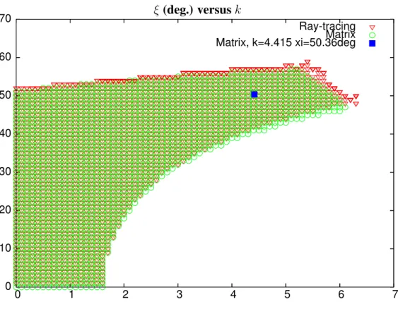
0 10 20 30 40 50 60 70 0 1 2 3 4 5 6 7 Ray-tracing Matrix Matrix, k=4.415 xi=50.36deg

Figure 8: k, ξstability domain. Circles : from matrix transport, triangles : from ray-tracing.

νz versus νr 0 1 2 3 4 5 0 1 2 3 4 5 Ray-tracing Matrix Matrix, k=4.415 xi=50.36deg

Figure 9: Tune diagram showing the periodic stability region. Circles : from matrix transport, triangles : from stepwise ray-tracing.

(11)

mesh size, integration step size. The third method has all the merits, speed, symplecticity, and its allowing automatic parameter fits.

3 Beam dynamics in a spiral ring

In this Section the numerical techniques described above are tested, with the goal of showing that this spiral magnet modelling allied with stepwise ray-tracing methods provide an efficient design tool. For that purpose a particular spiral FFAG geometry, representative of a protontherapy class machine, is submitted to various numerical experiments, as follows.

3.1 Magnet and ring geometry

The geometry and parameters of the N-sector lattice of concern are shown in Fig. 6. The magnets occupy a fraction (“packing factor”) pf = 0.38 of the circumference, independent of radius, a scaling property. The extreme radii and rigidities satisfy, another scaling property, Bρ2/ Bρ1 = (r2/r1)k+1. In the smooth

approximation, the dipole sector angle A (Fig. 2) and bend angle β = 2π/N are in the ratio pf ; the sector radius r and curvature radius ρ satisfy r sin(A/2) = ρ sin(β/2).

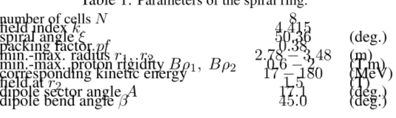
Table 1:Parameters of the spiral ring.

number of cells N 8

field index k 4.415

spiral angle ξ 50.36 (deg.)

packing factor pf 0.38

min.-max. radius r1, r2 2.78 − 3.48 (m)

min.-max. proton rigidity Bρ1, Bρ2 0.6 − 2. (T.m)

corresponding kinetic energy 17 − 180 (MeV)

field at r2 1.5 (T)

dipole sector angle A 17.1 (deg.)

dipole bend angle β 45.0 (deg.)

The smooth approximation allows deriving the optical functions on an arbitrary closed orbit (Fig. 7) with reasonable accuracy from matrix representation, with optical elements being the two end drifts r sin(π/N − A/2), dipole ends wedge angles ² En.Ex. = π/N − A/2 ± ξ, and the dipole body ρ, β.

A scan of the (k, ξ) space in the smooth approximation yields the stability region shown in Fig. 8 (cir-cles), and the corresponding tune domain shown in Fig. 9. A similar (k, ξ) scan using the ray-tracing method and field modelling described in Section 2 has been superimposed (triangles in Figs. 8, 9). The agreement between both methods is good for lower k and ξ values and deteriorates with increasing k and with increasing ξ - this behavior will be devoted further investigation, however it could be attributed to (i) the loss of validity of the constant orbit radius assumption in the smooth approximation, i.e. closed orbits in the dipole sensibly depart from an arc of a circle, and to (ii) the increasing perturbative effect of fringe fields, as they are traversed over an increasingly long distance for larger ξ values.

It can be concluded at that stage that the consistency of the two types of results is good, so confirming the efficiency of the smooth approximation for a first approach of the magnet and lattice parameters, whereas the precision of ray-tracing is necessary for further insight into ring design and beam dynamics.

3.2 First order behavior

In the beam dynamics studies that follow we consider for illustration the particular optics (k, ξ) = (4.415, 50.36deg.), subject to extensive studies in the frame of the RACCAM project [9, 10] (the working point materialized

by a square solid marker in Fig. 8). The corresponding tune values, using the FFAG-SPI method (respec-tively, in the matrix approximation) are (νr, νz) = (2.817, 1.793)(respectively (νr, νz) = (2.896, 1.952),

(12)

tional to radius (g0= 3cm at R0 ≡ r2= 3.48m, κ = −1 in Eq. 5) thus yielding very weak sensitivity of

vertical tune to radius1_{in addition to quasi-constant horizontal tune as ensuing from the property of zero}

chromaticity. Namely, the ray-tracing yields (νr, νz) = (2.817, 1.793)at better than ±3 10−4 (relative)

over the full radial extent [r1, r2] = [2.78m, 3.48m].

Fig. 10 shows the radius value (taken to the center of the ring) along closed orbits over the 2π/8 cell extent, at various momenta. It can be observed that the scaling rule r/R0= (p/p0)1/(k+1)is satisfied with

good precision ; indeed, inside the dipole (the θ regions with non-zero magnetic field, see Fig. 11), the closed orbit radius departs by no more than about ±3% from the theoretical, r = Cst _smooth

approxima-tion value. Fig. 11 shows the magnetic field along those closed orbits.

The momentum compaction α = dL/L / dp/p can be numerically computed from ∆p induced dif-ference in closed orbit lengths. Sample values are given in Fig. 12, they are close to the theoretical value α ≈ 1/(1 + K).

All these results show good consistency and reasonable agreement between the smooth approximation data and numerical results, a property useful in preliminary design stages.

3.3 Large amplitude motion

The main goal in this section is to show the satisfactory behavior of the numerical spiral magnet modelling, and of the large amplitude multiturn tracking.

Fig. 13 shows horizontal phase space trajectories at the limit of stable motion in the ring, for various energies, as observed along a radial direction in the drift region ; the triangle shape of phase space motion is related to the presence of strong sextupole component in B(r) (Eq. 2) and to the proximity to third integer cell tune ; the triangles rotate due to the change of focusing conditions along a radius (the focusing is invariant by a displacement ∆r, ∆θ = tan(ξ) ln((r + ∆r)/r)). Fig. 14 shows vertical phase space trajectories at the limit of stable motion in the ring, for three different energies, and with cell tune close to quarter integer.

Fig. 15 and Fig. 16 show horizontal and vertical phase space motion at 60 MeV, observed at the center of the drift ; the symplecticity is very good, up to stability limit. Another feature in these Figures is the large dynamical acceptance characteristic of FFAG optics : the surface of the 60 MeV stability limit portraits are ²r ≈ 1000π mm.mrad, ²r ≈ 200π mm.mrad. The corresponding amplitude detuning resulting from

the non-linear field is shown in Fig. 17.

Fig. 18 shows the tune footprint of a monochromatic beam with size ²r ≈ ²z≈ 100 π mm.rad, together

with right and skew systematic resonance lines up to 6th order. Automatized tracking tools have been developed to scan the dynamic aperture in the vicinity of the working point in the tune diagram [16], typical results are shown in Fig. 19. This method is now routinely used in the design of the spiral magnet in the frame of the RACCAM project [9, 10].

1_{In the smooth approximation, this can be understood from the vertical wedge focusing, namely (z}0_/z0

0) = tan(² − ψ)/ρ),

given the correction for the fringe field extent ψ = Ig ρ

1+sin2²

cos² , wherein I is a form factor, so that g v ρ = pf × r yields

(13)

-.6 -.4 -.2 0.0 0.2 2.7 2.8 2.9 3. 3.1 3.2 3.3 3.4 3.5 r (m) vs. (rad) θ 17 MeV 32 60 107 180 MeV

Figure 10:Radius value (taken to the center of the ring) along closed orbits, in a cell.

-.6 -.4 -.2 0.0 0.2 0.2 0.4 0.6 0.8 1. 1.2 1.4

* Data generated by searchCO * B (T) vs. (rad) θ 17 MeV 32 60 107 180 MeV

Figure 11:Magnetic field on closed orbits, along a cell.

0 10 20 30 40 50 0.2 0.4 0.6 0.8 1. 1.2 K = 0 K = 1 K = 2 K = 3 ₄ K = 5

vs. spiral angle (deg)

α

(14)

2.8 2.9 3. 3.1 3.2 3.3 0.0 0.05 0.1 0.15 0.2 0.25 0.3 r’ (rad) vs. r (m) 17 MeV 32 60 107 180 MeV

Figure 13: Horizontal stability limits, at 1 mm preci-sion, 1000 cells, for various energies.

-.04 -.02 0.0 0.02 0.04 -.01 0.0 0.01 0.02 180 MeV 60 17 MeV z’ (rad) vs. z (m)

Figure 14: Vertical stability limits, at 1 mm precision, 1000 cells. Horizontal motion is near closed orbit.

3.01 3.02 3.03 3.04 3.05 3.06 3.07 0.1 0.12 0.14 0.16 0.18 0.2 r’ (rad) vs. r (m) 60 MeV

Figure 15:60 MeV horizontal phase-space, up to ≈ 1000 π mm.mrad maximum stable amplitude.

-.03 -.02 -.01 0.0 0.01 0.02 0.03 -.015 -.01 -.005 0.0 0.005 0.01 0.015 z’ (rad) vs. z (m) 60 MeV

(15)

IN2P3 LPSC 07-40 14 1.6 1.8 2 2.2 2.4 2.6 2.8 3 3.2 0.2 0.4 0.6 0.8 1 Tunes Emittance/Emittance_max

Amplitude detuning

Qx vs. Em_x Qz vs. Em_z Qz vs. Em_x

Figure 17:Amplitude detuning, from paraxial motion up to maximum stable amplitude. 60 MeV case.

2.6 2.7 2.8 2.9 3. 1.6 1.65 1.7 1.75 1.8 1.85 1.9 1.95 2. TUNE DIAGRAM ν ν z x 3 3 3 4 5 5 6 6 6 6

Figure 18: Beam occupation in tune diagram, due to amplitude detuning (given δp/p ≡ 0, ²r ≈ ²z ≈

100 πmm.rad). Right + skew lines mνr+ nνz = pas well as |m| + |n| values are shown ; the two thick lines

are neighboring systematic resonances, 3νr= 8, 4νr− 2νz= 8, .

2.25 2.5 2.75 3 3.25 3.5 3.75 4 0.5 1 1.5 2 2.5 3 85,0,0< 85,0,0< 85,0,0< 85,0,0< 85,0,0< 85,0,0< 85,0,0< 85,0,0< 85,0,0< 85,0,0< 85,0,0< 85,0,0< 85,0,0< 85,0,0< 85,0,1< 85,0,1< 85,0,1< 85,0,1< 85,0,1< 85,0,1< 85,0,1< 85,0,1< 85,0,1< 85,0,1< 85,0,1< 85,0,2< 85,0,2< 85,0,2< 85,0,2< 85,0,2< 85,0,2< 85,0,2< 85,0,2< 85,0,2< 85,0,3< 85,0,3< 85,0,3< 85,0,3< 85,0,3< 85,0,3< 85,0,3< 81,4,0< _81,4,0< 81,4,0< _81,4,0< 81,4,0< _81,4,0< 81,4,0< _81,4,0< 81,4,0< _81,4,0< 81,4,0< _81,4,0< 81,4,0< _81,4,0< 81,4,1< 81,4,1< 81,4,1< _81,4,1< 81,4,1< 81,4,1< 81,4,1< 81,4,1< _81,4,1< 81,4,1< 81,4,1< 81,4,2< 81,4,2< 81,4,2< 81,4,2< 81,4,2< 81,4,2< 81,4,2< 81,4,2< 81,4,2< 81,4,3< 81,4,3< 81,4,3< 81,4,3< 81,4,3< 81,4,3< 81,4,3< 81,-4,0< 81,-4,0< 81,-4,0< 81,-4,0< 81,-4,0< 81,-4,0< 81,-4,0< 81,-4,0< 81,-4,0< 81,-4,0< 81,-4,0< 81,-4,0< 81,-4,0< 81,-4,0< 81,-4,1< 81,-4,1< 81,-4,1< 81,-4,1< 81,-4,1< 81,-4,1< 81,-4,1< 81,-4,1< 81,-4,1< 81,-4,1< 81,-4,1< 81,-4,2< 81,-4,2< 81,-4,2< 81,-4,2< 81,-4,2< 81,-4,2< 81,-4,2< 81,-4,2< 81,-4,2< 81,-4,3< 81,-4,3< 81,-4,3< 81,-4,3< 81,-4,3< 81,-4,3< 81,-4,3< 83,2,0< 83,2,0< 83,2,0< 83,2,0< 83,2,0< 83,2,0< 83,2,0< 83,2,0< 83,2,0< 83,2,0< 83,2,0< 83,2,0< 83,2,0< 83,2,0< 83,2,1< 83,2,1< 83,2,1< 83,2,1< 83,2,1< 83,2,1< 83,2,1< 83,2,1< 83,2,1< 83,2,1< 83,2,1< 83,2,2< 83,2,2< 83,2,2< 83,2,2< 83,2,2< 83,2,2< 83,2,2< 83,2,2< 83,2,2< 83,2,3< 83,2,3< 83,2,3< 83,2,3< 83,2,3< 83,2,3< 83,2,3< 83,-2,0< 83,-2,0< 83,-2,0< 83,-2,0< 83,-2,0< 83,-2,0< 83,-2,0< 83,-2,0< 83,-2,0< 83,-2,0< 83,-2,0< 83,-2,0< 83,-2,0< 83,-2,0< 83,-2,1< 83,-2,1< 83,-2,1< 83,-2,1< 83,-2,1< 83,-2,1< 83,-2,1< 83,-2,1< 83,-2,1< 83,-2,1< 83,-2,1< 83,-2,2< 83,-2,2< 83,-2,2< 83,-2,2< 83,-2,2< 83,-2,2< 83,-2,2< 83,-2,2< 83,-2,2< 83,-2,3< 83,-2,3< 83,-2,3< 83,-2,3< 83,-2,3< 83,-2,3< 83,-2,3< 84,0,0< 84,0,0< 84,0,0< 84,0,0< 84,0,0< 84,0,0< 84,0,0< 84,0,0< 84,0,0< 84,0,0< 84,0,0< 84,0,0< 84,0,0< 84,0,0< 84,0,1< 84,0,1< 84,0,1< 84,0,1< 84,0,1< 84,0,1< 84,0,1< 84,0,1< 84,0,1< 84,0,1< 84,0,1< 84,0,2< 84,0,2< 84,0,2< 84,0,2< 84,0,2< 84,0,2< 84,0,2< 84,0,2< 84,0,2< 84,0,3< 84,0,3< 84,0,3< 84,0,3< 84,0,3< 84,0,3< 84,0,3< 80,4,0< 80,4,0< 80,4,0< 80,4,0< 80,4,0< 80,4,0< 80,4,0< 80,4,0< 80,4,0< 80,4,0< 80,4,0< 80,4,0< 80,4,0< 80,4,0< 80,4,1< 80,4,1< 80,4,1< 80,4,1< 80,4,1< 80,4,1< 80,4,1< 80,4,1< 80,4,1< 80,4,1< 80,4,1< 80,4,2< 80,4,2< 80,4,2< 80,4,2< 80,4,2< 80,4,2< 80,4,2< 80,4,2< 80,4,2< 80,4,3< 80,4,3< 80,4,3< 80,4,3< 80,4,3< 80,4,3< 80,4,3< 82,-2,0< 82,-2,0< 82,-2,0< 82,-2,0< 82,-2,0< 82,-2,0< 82,-2,0< 82,-2,0< 82,-2,0< 82,-2,0< 82,-2,0< 82,-2,0< 82,-2,0< 82,-2,0< 82,-2,1< 82,-2,1< 82,-2,1< 82,-2,1< 82,-2,1< 82,-2,1< 82,-2,1< 82,-2,1< 82,-2,1< 82,-2,1< 82,-2,1< 82,-2,2< 82,-2,2< 82,-2,2< 82,-2,2< 82,-2,2< 82,-2,2< 82,-2,2< 82,-2,2< 82,-2,2< 82,-2,3< 82,-2,3< 82,-2,3< 82,-2,3< 82,-2,3< 82,-2,3< 82,-2,3< 82,2,0< 82,2,0< 82,2,0< 82,2,0< 82,2,0< 82,2,0< 82,2,0< 82,2,0< 82,2,0< 82,2,0< 82,2,0< 82,2,0< 82,2,0< 82,2,0< 82,2,1< 82,2,1< 82,2,1< 82,2,1< 82,2,1< 82,2,1< 82,2,1< 82,2,1< 82,2,1< 82,2,1< 82,2,1< 82,2,2< 82,2,2< 82,2,2< 82,2,2< 82,2,2< 82,2,2< 82,2,2< 82,2,2< 82,2,2< 82,2,3< 82,2,3< 82,2,3< 82,2,3< 82,2,3< 82,2,3< 82,2,3< 83,0,0< 83,0,0< 83,0,0< 83,0,0< 83,0,0< 83,0,0< 83,0,0< 83,0,0< 83,0,0< 83,0,0< 83,0,0< 83,0,0< 83,0,0< 83,0,0< 83,0,1< 83,0,1< 83,0,1< 83,0,1< 83,0,1< 83,0,1< 83,0,1< 83,0,1< 83,0,1< 83,0,1< 83,0,1< 83,0,2< 83,0,2< 83,0,2< 83,0,2< 83,0,2< 83,0,2< 83,0,2< 83,0,2< 83,0,2< 83,0,3< 83,0,3< 83,0,3< 83,0,3< 83,0,3< 83,0,3< 83,0,3< 81,2,0< 81,2,0< 81,2,0< 81,2,0< 81,2,0< 81,2,0< 81,2,0< 81,2,0< 81,2,0< 81,2,0< 81,2,0< 81,2,0< 81,2,0< 81,2,0< 81,2,1< 81,2,1< 81,2,1< 81,2,1< 81,2,1< 81,2,1< 81,2,1< 81,2,1< 81,2,1< 81,2,1< 81,2,1< 81,2,2< 81,2,2< 81,2,2< 81,2,2< 81,2,2< 81,2,2< 81,2,2< 81,2,2< 81,2,2< 81,2,3< 81,2,3< 81,2,3< 81,2,3< 81,2,3< 81,2,3< 81,2,3< 81,-2,0< 81,-2,0< 81,-2,0< 81,-2,0< 81,-2,0< 81,-2,0< 81,-2,0< 81,-2,0< 81,-2,0< 81,-2,0< 81,-2,0< 81,-2,0< 81,-2,0< 81,-2,0< 81,-2,1< 81,-2,1< 81,-2,1< 81,-2,1< 81,-2,1< 81,-2,1< 81,-2,1< 81,-2,1< 81,-2,1< 81,-2,1< 81,-2,1< 81,-2,2< 81,-2,2< 81,-2,2< 81,-2,2< 81,-2,2< 81,-2,2< 81,-2,2< 81,-2,2< 81,-2,2< 81,-2,3< 81,-2,3< 81,-2,3< 81,-2,3< 81,-2,3< 81,-2,3< 81,-2,3< 82,0,0< 82,0,0< 82,0,0< 82,0,0< 82,0,0< 82,0,0< 82,0,0< 82,0,0< 82,0,0< 82,0,0< 82,0,0< 82,0,0< 82,0,0< 82,0,0< 82,0,1< 82,0,1< 82,0,1< 82,0,1< 82,0,1< 82,0,1< 82,0,1< 82,0,1< 82,0,1< 82,0,1< 82,0,1< 82,0,2< 82,0,2< 82,0,2< 82,0,2< 82,0,2< 82,0,2< 82,0,2< 82,0,2< 82,0,2< 82,0,3< 82,0,3< 82,0,3< 82,0,3< 82,0,3< 82,0,3< 82,0,3< 80,2,0< 80,2,0< 80,2,0< 80,2,0< 80,2,0< 80,2,0< 80,2,0< 80,2,0< 80,2,0< 80,2,0< 80,2,0< 80,2,0< 80,2,0< 80,2,0< 80,2,1< 80,2,1< 80,2,1< 80,2,1< 80,2,1< 80,2,1< 80,2,1< 80,2,1< 80,2,1< 80,2,1< 80,2,1< 80,2,2< 80,2,2< 80,2,2< 80,2,2< 80,2,2< 80,2,2< 80,2,2< 80,2,2< 80,2,2< 80,2,3< 80,2,3< 80,2,3< 80,2,3< 80,2,3< 80,2,3< 80,2,3< 81,0,0< 81,0,0< 81,0,0< 81,0,0< 81,0,0< 81,0,0< 81,0,0< 81,0,0< 81,0,0< 81,0,0< 81,0,0< 81,0,0< 81,0,0< 81,0,0< 81,0,1< 81,0,1< 81,0,1< 81,0,1< 81,0,1< 81,0,1< 81,0,1< 81,0,1< 81,0,1< 81,0,1< 81,0,1< 81,0,2< 81,0,2< 81,0,2< 81,0,2< 81,0,2< 81,0,2< 81,0,2< 81,0,2< 81,0,2< 2.25 2.5 2.75 3 3.25 3.5 3.75 4 0.5 1 1.5 2 2.5 3 85,0,0< 85,0,0< 85,0,0< 85,0,0< 85,0,0< 85,0,0< 85,0,0< 85,0,0< 85,0,0< 85,0,0< 85,0,0< 85,0,0< 85,0,0< 85,0,0< 85,0,1< 85,0,1< 85,0,1< 85,0,1< 85,0,1< 85,0,1< 85,0,1< 85,0,1< 85,0,1< 85,0,1< 85,0,1< 85,0,2< 85,0,2< 85,0,2< 85,0,2< 85,0,2< 85,0,2< 85,0,2< 85,0,2< 85,0,2< 85,0,3< 85,0,3< 85,0,3< 85,0,3< 85,0,3< 85,0,3< 85,0,3< 81,4,0< _81,4,0< 81,4,0< _81,4,0< 81,4,0< _81,4,0< 81,4,0< _81,4,0< 81,4,0< _81,4,0< 81,4,0< _81,4,0< 81,4,0< _81,4,0< 81,4,1< 81,4,1< 81,4,1< _81,4,1< 81,4,1< 81,4,1< 81,4,1< 81,4,1< _81,4,1< 81,4,1< 81,4,1< 81,4,2< 81,4,2< 81,4,2< 81,4,2< 81,4,2< 81,4,2< 81,4,2< 81,4,2< 81,4,2< 81,4,3< 81,4,3< 81,4,3< 81,4,3< 81,4,3< 81,4,3< 81,4,3< 81,-4,0< 81,-4,0< 81,-4,0< 81,-4,0< 81,-4,0< 81,-4,0< 81,-4,0< 81,-4,0< 81,-4,0< 81,-4,0< 81,-4,0< 81,-4,0< 81,-4,0< 81,-4,0< 81,-4,1< 81,-4,1< 81,-4,1< 81,-4,1< 81,-4,1< 81,-4,1< 81,-4,1< 81,-4,1< 81,-4,1< 81,-4,1< 81,-4,1< 81,-4,2< 81,-4,2< 81,-4,2< 81,-4,2< 81,-4,2< 81,-4,2< 81,-4,2< 81,-4,2< 81,-4,2< 81,-4,3< 81,-4,3< 81,-4,3< 81,-4,3< 81,-4,3< 81,-4,3< 81,-4,3< 83,2,0< 83,2,0< 83,2,0< 83,2,0< 83,2,0< 83,2,0< 83,2,0< 83,2,0< 83,2,0< 83,2,0< 83,2,0< 83,2,0< 83,2,0< 83,2,0< 83,2,1< 83,2,1< 83,2,1< 83,2,1< 83,2,1< 83,2,1< 83,2,1< 83,2,1< 83,2,1< 83,2,1< 83,2,1< 83,2,2< 83,2,2< 83,2,2< 83,2,2< 83,2,2< 83,2,2< 83,2,2< 83,2,2< 83,2,2< 83,2,3< 83,2,3< 83,2,3< 83,2,3< 83,2,3< 83,2,3< 83,2,3< 83,-2,0< 83,-2,0< 83,-2,0< 83,-2,0< 83,-2,0< 83,-2,0< 83,-2,0< 83,-2,0< 83,-2,0< 83,-2,0< 83,-2,0< 83,-2,0< 83,-2,0< 83,-2,0< 83,-2,1< 83,-2,1< 83,-2,1< 83,-2,1< 83,-2,1< 83,-2,1< 83,-2,1< 83,-2,1< 83,-2,1< 83,-2,1< 83,-2,1< 83,-2,2< 83,-2,2< 83,-2,2< 83,-2,2< 83,-2,2< 83,-2,2< 83,-2,2< 83,-2,2< 83,-2,2< 83,-2,3< 83,-2,3< 83,-2,3< 83,-2,3< 83,-2,3< 83,-2,3< 83,-2,3< 84,0,0< 84,0,0< 84,0,0< 84,0,0< 84,0,0< 84,0,0< 84,0,0< 84,0,0< 84,0,0< 84,0,0< 84,0,0< 84,0,0< 84,0,0< 84,0,0< 84,0,1< 84,0,1< 84,0,1< 84,0,1< 84,0,1< 84,0,1< 84,0,1< 84,0,1< 84,0,1< 84,0,1< 84,0,1< 84,0,2< 84,0,2< 84,0,2< 84,0,2< 84,0,2< 84,0,2< 84,0,2< 84,0,2< 84,0,2< 84,0,3< 84,0,3< 84,0,3< 84,0,3< 84,0,3< 84,0,3< 84,0,3< 80,4,0< 80,4,0< 80,4,0< 80,4,0< 80,4,0< 80,4,0< 80,4,0< 80,4,0< 80,4,0< 80,4,0< 80,4,0< 80,4,0< 80,4,0< 80,4,0< 80,4,1< 80,4,1< 80,4,1< 80,4,1< 80,4,1< 80,4,1< 80,4,1< 80,4,1< 80,4,1< 80,4,1< 80,4,1< 80,4,2< 80,4,2< 80,4,2< 80,4,2< 80,4,2< 80,4,2< 80,4,2< 80,4,2< 80,4,2< 80,4,3< 80,4,3< 80,4,3< 80,4,3< 80,4,3< 80,4,3< 80,4,3< 82,-2,0< 82,-2,0< 82,-2,0< 82,-2,0< 82,-2,0< 82,-2,0< 82,-2,0< 82,-2,0< 82,-2,0< 82,-2,0< 82,-2,0< 82,-2,0< 82,-2,0< 82,-2,0< 82,-2,1< 82,-2,1< 82,-2,1< 82,-2,1< 82,-2,1< 82,-2,1< 82,-2,1< 82,-2,1< 82,-2,1< 82,-2,1< 82,-2,1< 82,-2,2< 82,-2,2< 82,-2,2< 82,-2,2< 82,-2,2< 82,-2,2< 82,-2,2< 82,-2,2< 82,-2,2< 82,-2,3< 82,-2,3< 82,-2,3< 82,-2,3< 82,-2,3< 82,-2,3< 82,-2,3< 82,2,0< 82,2,0< 82,2,0< 82,2,0< 82,2,0< 82,2,0< 82,2,0< 82,2,0< 82,2,0< 82,2,0< 82,2,0< 82,2,0< 82,2,0< 82,2,0< 82,2,1< 82,2,1< 82,2,1< 82,2,1< 82,2,1< 82,2,1< 82,2,1< 82,2,1< 82,2,1< 82,2,1< 82,2,1< 82,2,2< 82,2,2< 82,2,2< 82,2,2< 82,2,2< 82,2,2< 82,2,2< 82,2,2< 82,2,2< 82,2,3< 82,2,3< 82,2,3< 82,2,3< 82,2,3< 82,2,3< 82,2,3< 83,0,0< 83,0,0< 83,0,0< 83,0,0< 83,0,0< 83,0,0< 83,0,0< 83,0,0< 83,0,0< 83,0,0< 83,0,0< 83,0,0< 83,0,0< 83,0,0< 83,0,1< 83,0,1< 83,0,1< 83,0,1< 83,0,1< 83,0,1< 83,0,1< 83,0,1< 83,0,1< 83,0,1< 83,0,1< 83,0,2< 83,0,2< 83,0,2< 83,0,2< 83,0,2< 83,0,2< 83,0,2< 83,0,2< 83,0,2< 83,0,3< 83,0,3< 83,0,3< 83,0,3< 83,0,3< 83,0,3< 83,0,3< 81,2,0< 81,2,0< 81,2,0< 81,2,0< 81,2,0< 81,2,0< 81,2,0< 81,2,0< 81,2,0< 81,2,0< 81,2,0< 81,2,0< 81,2,0< 81,2,0< 81,2,1< 81,2,1< 81,2,1< 81,2,1< 81,2,1< 81,2,1< 81,2,1< 81,2,1< 81,2,1< 81,2,1< 81,2,1< 81,2,2< 81,2,2< 81,2,2< 81,2,2< 81,2,2< 81,2,2< 81,2,2< 81,2,2< 81,2,2< 81,2,3< 81,2,3< 81,2,3< 81,2,3< 81,2,3< 81,2,3< 81,2,3< 81,-2,0< 81,-2,0< 81,-2,0< 81,-2,0< 81,-2,0< 81,-2,0< 81,-2,0< 81,-2,0< 81,-2,0< 81,-2,0< 81,-2,0< 81,-2,0< 81,-2,0< 81,-2,0< 81,-2,1< 81,-2,1< 81,-2,1< 81,-2,1< 81,-2,1< 81,-2,1< 81,-2,1< 81,-2,1< 81,-2,1< 81,-2,1< 81,-2,1< 81,-2,2< 81,-2,2< 81,-2,2< 81,-2,2< 81,-2,2< 81,-2,2< 81,-2,2< 81,-2,2< 81,-2,2< 81,-2,3< 81,-2,3< 81,-2,3< 81,-2,3< 81,-2,3< 81,-2,3< 81,-2,3< 82,0,0< 82,0,0< 82,0,0< 82,0,0< 82,0,0< 82,0,0< 82,0,0< 82,0,0< 82,0,0< 82,0,0< 82,0,0< 82,0,0< 82,0,0< 82,0,0< 82,0,1< 82,0,1< 82,0,1< 82,0,1< 82,0,1< 82,0,1< 82,0,1< 82,0,1< 82,0,1< 82,0,1< 82,0,1< 82,0,2< 82,0,2< 82,0,2< 82,0,2< 82,0,2< 82,0,2< 82,0,2< 82,0,2< 82,0,2< 82,0,3< 82,0,3< 82,0,3< 82,0,3< 82,0,3< 82,0,3< 82,0,3< 80,2,0< 80,2,0< 80,2,0< 80,2,0< 80,2,0< 80,2,0< 80,2,0< 80,2,0< 80,2,0< 80,2,0< 80,2,0< 80,2,0< 80,2,0< 80,2,0< 80,2,1< 80,2,1< 80,2,1< 80,2,1< 80,2,1< 80,2,1< 80,2,1< 80,2,1< 80,2,1< 80,2,1< 80,2,1< 80,2,2< 80,2,2< 80,2,2< 80,2,2< 80,2,2< 80,2,2< 80,2,2< 80,2,2< 80,2,2< 80,2,3< 80,2,3< 80,2,3< 80,2,3< 80,2,3< 80,2,3< 80,2,3< 81,0,0< 81,0,0< 81,0,0< 81,0,0< 81,0,0< 81,0,0< 81,0,0< 81,0,0< 81,0,0< 81,0,0< 81,0,0< 81,0,0< 81,0,0< 81,0,0< 81,0,1< 81,0,1< 81,0,1< 81,0,1< 81,0,1< 81,0,1< 81,0,1< 81,0,1< 81,0,1< 81,0,1< 81,0,1< 81,0,2< 81,0,2< 81,0,2< 81,0,2< 81,0,2< 81,0,2< 81,0,2< 81,0,2< 81,0,2<

Figure 19:A scan of the dynamic aperture in the (νr, νz) = (2.8, 1.8)region, (a) in case of horizontal motion with

(16)

An RF gap is now introduced in the ring, as represented in Fig. 20. -4 -3 -2 -1 0 1 2 3 4 5 -3 -2 -1 0 1 2 3 (m) (m)

Figure 20:Positioning of the RF gap in a drift.

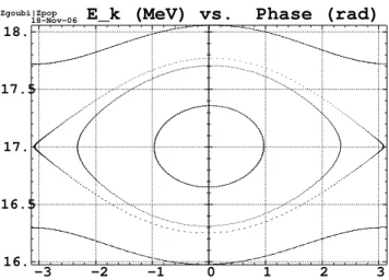
4.1 Stationary bucket

The RF gap is located in a drift, along a radius, orthogonal to the maximum energy closed orbit (r ≈ 3.4 m, see Fig. 20). Injection orbit, 17 MeV, γ = 1.01812, r ≈ 2.75 m, 17.33 m circumference, is considered. The peak RF voltage is ˆV = 20kV, a value rather large for the sake of faster tracking. Other RF parameters are, fRF = 3.249 MHz, harmonic=1, synchronous phase φs = 0. These conditions yield theoretical

momentum acceptance ±∆p p = ± 1 βs Ã 2q ˆV πhηEs !1/2 ≈ ±2.18 % (8)

given Es = 955.27MeV synchronous energy, slippage factor η = _γ12 − α = _γ12 − _1+K1 ≈ 0.78 with

K = 4.415. The theoretical small amplitude synchrotron tune is νs= 1 β Ã hη cos φsq ˆV 2πEs !1/2 ≈ 8.52 10−3 (9)

Both ∆p/p and νs values are in excellent agreement with values of bucket height and RF cycles per

turn obtained from numerical simulations as shown in Fig. 21, namely ±∆p/p = ±2.20% and νs =

1/117turns.

4.2 A full acceleration cycle

A particle is now launched with all starting coordinates zero except for z0 = 3mm.

From 17 to 180 MeV, the RF frequency is increased linearly with turn number from 3.25 to 7.51 MHz, at constant synchronous phase φs= 30degrees, ˆV = 20kV, which means about 16000 turns to complete

the cycle.

Fig. 22 shows the first synchrotron oscillation cycles, from 17 to 18.47 MeV, of ±1% off-momentum particles around a quasi-synchronous one. From the figure, the synchrotron period appears to be in agree-ment with Eq. 9, given the working hypothesis above.

(17)

-3 -2 -1 0 1 2 3 16. 16.5 17. 17.5 18. Zgoubi|Zpop 18-Nov-06

* Data generated by geneMap. K= 3.5 xi= 50. deg * E_k (MeV) vs. Phase (rad)

Min-max. Hor.: -3.141 3.141 ; Ver.: 15.98 18.06 Part# 1-40000 (*) ; Lmnt# 1; pass# 1- 604; 3020 points Figure 21:Stationary bucket on injection orbit.

50 100 150 200 250 300 350 400 17. 17.5 18. 18.5 Zgoubi|Zpop 28-Apr-07

* Data generated by searchCO * KinEnr (MeV) vs. Pass#

Min-max. Hor.: 1.000 400.0 ; Ver.: 16.67 18.72 Part# 1- 1 (*) ; Lmnt# 1; pass# 1- 400; 400 points

Zgoubi|Zpop 28-Apr-07

Min-max. Hor.: 1.000 400.0 ; Ver.: 16.67 18.72 Part# 2- 2 (*) ; Lmnt# 1; pass# 1- 400; 400 points

Zgoubi|Zpop 28-Apr-07

Min-max. Hor.: 1.000 400.0 ; Ver.: 16.67 18.72 Part# 3- 3 (*) ; Lmnt# 1; pass# 1- 400; 400 points Figure 22:First 400 turns of an acceleration cycle in the 8-cell spiral ring. dp/p ≈ 10−3and ±1%.

(18)

2.8 2.9 3. 3.1 3.2 3.3 -.006 -.004 -.002 0.0 0.002 0.004 0.006

* Data generated by searchCO * Figure 23:Adiabatic damping of vertical motion over an acceleration cycle.

-.006 -.004 -.002 0.0 0.002 0.004 0.006 -.003 -.002 -.001 0.0 0.001 0.002 0.003 0.004 Zgoubi|Zpop 2-May-07 Z’ (rad) vs. Z (m) 17 MeV 170 MeV

Figure 24: Adiabatic damping of vertical motion over an acceleration cycle (transverse phase space observed at fixed azimuth). Larger amplitude (resp. smaller) corresponds to injection (resp. final) energy.

Sample vertical motion is displayed in Figs. 23, 24 and shows excellent behavior. Regular damping can be observed, of the form (Bρ₁₇₀_MeV/Bρ₁₇_MeV)1/2 _≈√3.3from start to end of the cycle. Referring to Fig. 24, it yields a surface ratio of about 0.55 between the outer (17 MeV) ellipse and the inner one (170 MeV). Note that the ellipse rotates, since the observation is at fixed azimuth, as already pointed out concerning Figs. 13, 14.

4.3 Admittance at injection

Acceleration of 8000 particles over about 300 turns (from 17 MeV to about 18.1 MeV) is now performed. Acceleration conditions are the same as previously, Sec. 4.2. A 4-D mono-energetic bunch is considered, with transverse emittances far beyond dynamical aperture and non-correlated x − z coordinates. In these conditions the bunch will be cleaned from all particles beyond 4-D dynamical aperure ; a few hundred turns is sufficient to ensure that cleaning, particle loss beyond that will not be significant, given that the optics does not strongly change in the course of acceleration as can be seen in Figs. 13, 14. The about 2003/8000 surviving particles give a reasonable image of the ring admittance at injection, which can be observed, in Figs. 25, 26, to be about

(19)

not so far from single energy estimates in Sec. 3.3 (Figs. 13-16). 2.74 2.76 2.78 2.8 2.82 2.84 0.2 0.22 0.24 0.26 0.28 0.3 0.32 0.34

* Data generated by searchCO * r’ (rad) vs. r (m)

Min-max. Hor.: 2.740 2.840 ; Ver.: 0.2000 0.3400 Part# 1-40000 (*) ; Lmnt# 1; pass# 300- 300; 2003 points Figure 25: Horizontal admittance, 4-D case. Surface :

Ar/π ≈ 900 10− 6 m.rad. -.03 -.02 -.01 0.0 0.01 0.02 0.03 -.02 -.015 -.01 -.005 0.0 0.005 0.01 0.015 0.02 Z’ (rad) vs. Z (m)

Min-max. Hor.: -3.5000E-02 3.5000E-02; Ver.: -2.2000E-02 2.2000E-02 Part# 1-40000 (*) ; Lmnt# 1; pass# 300- 300; 2003 points Figure 26: Vertical admittance, 4-D case. Az/π ≈

190 10−6m.rad.

5 Conclusion

The developement of precision tracking tools presented here, a follow-on of an earlier work concerning radial FFAG lattice design [12], yields computing means now extensively used for spiral FFAG design [10]. In particular, they allow (i) providing benchmarking data in magnet design studies, and (ii) automatized matching of magnet and lattice parameters.

Not addressed here, automatized procedures for the injection of various type of defects (field, aligne-ment, etc.) have been developped that allow statistical analysis and tolerance evaluations [17].

The code developped for this purpose, Zgoubi [11], also provides ray-tracing in 2-D and 3-D magnetic field maps, it can therefore as well be used as the ultimate design and beam dynamics studies tool prior to construction.

References

[1] The rebirth of the FFAG, M. Craddock, CERN Courrier 44-6 (2004) ;

see also, Fixed field alternating gradient synchrotrons, F. M´eot, Invited talk, ICFA-HB2004 Workshop, Ben-sheim, 18-22 Oct. 2004.

[2] A feasibility study of a neutrino factory in Japan, KEK report, Feb. 2001.

[3] Feasibility Study-II of a Muon-Based Neutrino Source, ed., S. Ozaki et als., BNL-52623 (2001).

[4] Non-Scaling FFAGs for Radio-Isotopes Production, A.G. Ruggiero ; Non-scaling FFAG lattice de-sign for the Radioactive Ion Accelerator, D. Trbojevic, FFAG 2007 Workshop, LPSC, Grenoble. http://lpsc.in2p3.fr/congres/FFAG07/.

[5] Accelerator Design and Construction for FFAG-KUCA ADSR, Y. Ishi, FFAG04 workshop, KEK, Tsukuba, http://hadron.kek.jp/FFAG/FFAG04 HP/index.html.

[6] 10 MW Non-scaling, non-linear FFAG SNS, G.H. Rees, FFAG 2007 Workshop, LPSC, Grenoble. http://lpsc.in2p3.fr/congres/FFAG07/.

[7] Development of FFAG accelerators and their applications for intense secondary particle production, Y. Mori, NIM A 562-2, 23 June 2006, 591-595.

[8] Study of Compact Medical FFAG Accelerators, Toshiyuki Misu, FFAG04 workshop, KEK, Tsukuba, http://hadron.kek.jp/FFAG/FFAG04 HP/index.html.

(20)

[11] (a) The ray-tracing code Zgoubi, F. M´eot, NIM A 427 (1999) 353-356, and also

(b) Zgoubi users’ guide, F. M´eot and S. Valero, CEA DAPNIA SEA-97-13 and FERMILAB-TM-2010 (1997). [12] Developments in the ray-tracing code Zgoubi for 6-D multiturn tracking in FFAG rings, F. M´eot, F. Lemuet,

NIM A 547 (2005) 638-651 ;

see also, Status of 6-D transmission simulations in FFAGs, F. M´eot, FFAG05 Wrkshp, KURRI Institute, Kyoto, 5-9 Dec. 2005.

[13] FFAG Particle Accelerators, K. R. Symon et als., Phys. Rev. 103 (6), 1837 (1956).

[14] Deflecting magnets, H.A. Enge, in Focusing of charged particles, Vol. 2, A. Septier ed., Academic Press, New-York and London (1967).

[15] Optics and magnetic field map for a spiral FFAG, Florence Martinache, int. report IN2P3/LPSC, Grenoble (2006).

[16] Ray-tracing simulations in spiral sector FFAG magnets using Zgoubi code, J. Fourrier, int. report IN2P3/LPSC, Grenoble (2007).

See also, FFAG 2007 Workshophttp : //lpsc.in2p3.fr/congres/FFAG07/.