HAL Id: inria-00328990
https://hal.inria.fr/inria-00328990
Submitted on 10 Oct 2008
HAL is a multi-disciplinary open access
archive for the deposit and dissemination of
sci-entific research documents, whether they are
pub-lished or not. The documents may come from
teaching and research institutions in France or
abroad, or from public or private research centers.
L’archive ouverte pluridisciplinaire HAL, est
destinée au dépôt et à la diffusion de documents
scientifiques de niveau recherche, publiés ou non,
émanant des établissements d’enseignement et de
recherche français ou étrangers, des laboratoires
publics ou privés.
from a sequence of images
Didier Auroux, Jérôme Fehrenbach
To cite this version:
Didier Auroux, Jérôme Fehrenbach. Identification of velocity fields for geophysical fluids from a
sequence of images. Experiments in Fluids, Springer Verlag (Germany), 2011, 50 (2), pp.313-328.
�inria-00328990�
a p p o r t
d e r e c h e r c h e
N 0 2 4 9 -6 3 9 9 IS R N IN R IA /R R --6 6 7 5 --F R + E N G Thème NUMIdentification of velocity fields for geophysical fluids
from a sequence of images
Didier Auroux — Jérôme Fehrenbach
N° 6675
Centre de recherche INRIA Grenoble – Rhône-Alpes 655, avenue de l’Europe, 38334 Montbonnot Saint Ismier
fluids from a sequence of images
Didier Auroux
∗†, J´
erˆ
ome Fehrenbach
∗Th`eme NUM — Syst`emes num´eriques ´
Equipe-Projet MOISE
Rapport de recherche n°6675 — Octobre 2008 — 27 pages
Abstract: We propose an algorithm to estimate the motion between two
images. This algorithm is based on the nonlinear brightness constancy assump-tion. The number of unknowns is reduced by considering displacement fields that are piecewise linear with respect to each space variable, and the Jacobian matrix of the cost function to be minimized is assembled rapidly using a finite element method. Different regularization terms are considered, and a multiscale approach provides fast and efficient convergence properties. Several numerical results of this algorithm on simulated and real geophysical flows are presented and discussed.
Key-words: velocity field, sequence of images, identification process, constant
brightness assumption, nonlinear minimization, multigrid approach
∗ Institut de Math´ematiques de Toulouse, Universit´e Paul Sabatier Toulouse 3, 31062
Toulouse cedex 9, France (auroux@math.univ-toulouse.fr)
s´
equences d’images pour les fluides g´
eophysiques
R´esum´e : Nous proposons un algorithme pour estimer le d´eplacement entre
deux images. Cet algorithme est bas´e sur l’hypoth`ese de conservation de l’intensit´e lumineuse. Le nombre d’inconnues est r´eduit en consid´erant des champs de
d´eplacement affines par morceaux par rapport `a chaque variable d’espace, et
la matrice Jacobienne de la fonction coˆut `a minimiser est assembl´ee
rapide-ment grˆace `a une m´ethode d’´el´ements finis. Diff´erents termes de r´egularisation
sont ´etudi´es, et une approche multi-grille permet `a l’algorithme de converger
rapidement et efficacement. Plusieurs r´esultats num´eriques sont pr´esent´es et comment´es, sur des images de fluides g´eophysiques simul´ees et r´eelles.
Mots-cl´es : champs de vitesse, s´equences d’images, identification,
1
Introduction
Estimating the motion of a fluid is of great interest, particularly in geophysics where the fluid can be the ocean. Applications of the motion estimation in this domain include the assimilation of images data in oceanographic models, and a possible improvement of the forecasts. Indeed, the poor predictability of extreme
geophysical events (e.g. El Ni˜no for the ocean) has dramatic consequences.
These events are usually visible on satellite images several days before they become extreme, but they are generally not used for forecast, and these data are not considered within the data assimilation process. Such satellite images contain a huge amount of data, that should be assimilated in order to improve the forecast quality.
The numerical forecast of geophysical fluids is extremely difficult, mainly because they are governed by the general nonlinear equations of fluid dynamics. Such nonlinearities are source of a huge sensitivity to the initial conditions, and then an ultimate theoretical limit to deterministic prediction. This limit is still far from being reached, and substantial gain can still be obtained in the quality of forecasts. Over the past 20 years, observations of ocean and atmosphere circulation have become much more readily available, as a result of new satellite techniques. For example, the use of altimeter measurements has provided extremely valuable information about the sea-surface height, but very few observations of the dynamics and the velocity fields of the oceans are currently available, and hence assimilated.
The huge amount of information provided by satellite images must therefore be exploited, as more and more space-borne observations of increasing qual-ity are available. Ocean observations are provided by AVHRR, Modis, . . . , and dynamic observations of the atmosphere are provided by operational me-teorological satellites, in geostationary (Meteosat, GOES, GMS, . . . ) or polar (AVHRR, MetOp) orbit [6].
Several ideas have been very recently developed to assimilate image data. A first idea consists of identifying some characteristic structures in the image and then tracking them in time. This is currently developed in meteorology, using an adaptive thresholding technique for radiance temperatures in order to identify and track several cells [23]. Another idea is to consider a dual problem and to create some model images, coming from the numerical model itself, and to compare the satellite images with these model images, using for example a curvlet approach [21]. The main difficulty comes from the definition of an image model, able to create a synthetic image from a numerical model solution [16, 17]. The main concept of this paper is to define a fast and efficient way to iden-tify, or extract, velocity fields from several images (or a complete sequence of images). Assuming this point, we would then be able to obtain billions of pseudo-observations, corresponding to the extracted velocity fields, that could be considered in the usual data assimilation processes. The main advantage of such an approach is to provide a lot of information on the velocity, which is a state variable of all geophysical models, as it is much more easy to assimilate data that are directly related to the state variables. We should mention that a satellite image can have a resolution of 5000 × 5000 pixels, and that some satellites transmit such images every 15 to 30 minutes [14]. We propose in this paper a way to identify one velocity vector for each pixel of the image. Then, if we consider the meteorological case, in which periods of 6 hours are
consid-ered, the amount of information that can be extracted from the images of one meteorological satellite (nearly half a billion pixels) is at least 10 times larger than the currently assimilated data. Of course, we will see that all the identi-fied velocity fields are not reliable, mainly when there is no visible characteristic phenomenon, but we should be able to provide an amount of information that is comparable to the currently assimilated observations.
The hypothesis that is underlying this work is that the grey level of the points are preserved during the motion, this is known as the constant brightness hypothesis. The constant brightness hypothesis was introduced in [15], and the linearized equation derived from this hypothesis is the cornerstone of optical flow methods [20, 3, 4].
This hypothesis is justified here in the framework of oceanography, as the objet of interest, allowing us to track the fluid and identify its velocity, is usually a passive tracer, at least on relative short time periods: chlorophyll, sea surface temperature, chemical pollutants (e.g. hydrocarbons). . . All these tracers do not interact with the water on a short time period, and they are passively transported by the fluid.
Fluid motion estimation was considered by numerous authors for several years. An established technique for experimental measurements is particle imag-ing velocimetry (PIV), where tracer particles are included inside the flow, and spatio-temporal cross-correlation techniques are used to estimate the motion of sub-windows of the domain. The quite large size of the interrogation windows usually implies some poor local motion estimation, as several particles with different velocities are present [1, 7].
A variational approach is presented in [2] where a cost function similar to ours is minimized in the context of incompressible fluids, but an initial guess provided by cross-correlation is required. Some authors replace the constant brightness assumption by an integrated continuity equation [12, 8] in order to take into account the spreading of intensity sources. In [9] a small number of vortex and source particles that describe the motion are retrieved.
Several approaches have also been specifically proposed for the estimation of fluid flow velocity, based on models derived from the physical laws governing fluid mechanics (e.g. the continuity equation) [11, 18, 8]. Several regularizations have also been studied, from standard first order norms to second order div-curl operators.
We propose here to use an integrated version of the constant brightness hypothesis. Instead of linearizing the constant brightness hypothesis like in standard optical flow techniques, we define a nonlinear cost function that takes into account the fact that time sampling occurs at a finite rate. Moreover, the combination of bilinear interpolation of gray-levels with spatial regularization provides an accurate estimation of sub-pixel motion.
The cost function obtained from the integrated constant brightness assump-tion is minimized in nested subspaces of admissible displacement vector fields. The vector fields that we consider are piecewise linear with respect to each space variable, on squares defined by a grid. This grid is iteratively refined, and at each level the optimal displacement field is estimated rapidly since the Jaco-bian of the cost function is assembled using a finite-element method (only one reading of the data is required).
This paper is organized as follows. In section 2, we present a description of our algorithm with different regularization terms, a way to consider a multiscale
approach, and an estimator of the quality of the results. Then in section 3 we present the results of extensive numerical experiments on simulated data. Section 4 is devoted to numerical results on two different kinds of real data. Finally, some concluding remarks and perspectives are given in section 5.
2
Description of the algorithm
This section is devoted to the description of the algorithm that we use.
2.1
Nonlinear cost function
The velocity estimation relies on the following hypothesis: the brightness of the points does not change between successive frames (at least when the time step between successive images is small enough). Let Ω denote the rectangular
domain where the images are defined. The motion between the instants t0 and
t1 where the images are I0 and I1 is then the vector field (u, v) such that for
every point (x, y) ∈ Ω,
I1(x + u(x, y), y + v(x, y)) = I0(x, y). (1)
A vector field satisfying equation (1) is not unique, this is known as the aperture problem in optical flow. Moreover, measurements error make the equality (1) unlikely to be strictly satisfied. We propose a least squares optimization to replace the exact equality (1).
Denote L the set of Lipschitz vector fields. Consider the following function:
F (I0, I1; u, v)(x, y) = I1(x + u(x, y), y + v(x, y)) − I0(x, y), (2)
where the vector field (u, v) ∈ L and the images I0 and I1 are continuously
differentiable.
The map F is differentiable with respect to (u, v), and for (u, v) ∈ L and
d= (du, dv) ∈ L,
DF (u, v).d(x, y) = ∇I1(x + u(x, y), y + v(x, y)).d(x, y).
The optimal displacement vector field between the images I0 and I1
mini-mizes the following cost-function:
J(u, v) = 1 2 Z Ω [F (I0, I1; u, v)(x, y)]2 dx dy +1 2αR(u, v), (3)
where R(u, v) is a spatial regularization term and α is the regularization factor. Our numerical experiments used different spatial regularization terms, these are described in subsection 2.2 below.
The minimum of J is estimated in a nested sequence of subspaces of L. On a small dimensional subspace, the optimization is efficient and the algorithm is not trapped in local minima. The result is used as initial guess to minimize J in a larger subspace. The subspaces and the minimization strategy are described in subsection 2.3.
2.2
Regularization
The following regularization terms were used in our numerical experiments. In
these definitions, k . k represents the L2 norm of a scalar or vector field on the
image.
R0(u, v) = kuk2+ kvk2, (4)
R1(u, v) = k∇uk2+ k∇vk2= k∂xuk2+ k∂yuk2 (5)
+ k∂xvk2+ k∂xvk2,
Rdiv(u, v) = kdiv(u, v)k2= k∂xu + ∂yvk2, (6)
Rcurl(u, v) = kcurl(u, v)k2= k∂yu − ∂xvk2, (7)
Rdiv/curl(u, v) = kdiv(u, v)k2+ kcurl(u, v)k2 (8)
= k∂xu + ∂yvk2+ k∂yu − ∂xvk2,
R∇div(u, v) = k∇div(u, v)k2= k∂2xxu + ∂xy2 vk2+ k∂xy2 u + ∂yy2 vk2,(9)
R∇div/∇curl(u, v) = k∇div(u, v)k2+ k∇curl(u, v)k2 (10)
= k∂xx2 u + ∂xy2 vk2+ k∂xy2 u + ∂yy2 vk2
+ k∂xy2 u − ∂xx2 vk2+ k∂yy2 u − ∂xy2 vk2.
In all the cases, the regularization term is the square of the image of (u, v) by a linear operator S. Below, the unifying following notation is used:
R(u, v) = ||S(u, v)||2,
where S is a linear operator. Some scalar coefficients have also been considered in order to weight the different terms of a given regularization.
2.3
Multiscale approach and optimization
The minimization of the cost-function J is performed in nested subspaces:
C16⊂ C8⊂ C4⊂ C2⊂ C1,
where the set Cq of admissible displacement fields at the scale q contains
piece-wise affine vector fields with respect to each space variable, on squares of size q × q pixels. We present and adapt here the method that was introduced in [10]. The difference with hierarchical techniques issued from the optical flow family (e.g. [22, 24]) is that we do not linearize the cost function. This should help to find large displacements, where the domain of linearity of the luminance function is not valid. Another innovation of the present work is the efficient
computation of the product DFTDF of the Jacobian of the first term of the
cost function (3) by its transpose. This efficient computation comes from the observation that this matrix is sparse and can be assembled like a finite-element matrix using one loop over the data.
The space C16 is typically of small dimension, hence the minimization of J
on C16 is fast and robust when a zero vector field is used as initial guess. The
optimal vector field obtained at a given scale in the space Cq is used as initial
We assume for simplicity that the dimensions (n, m) of the images satisfy n = 16N + 1 and m = 16M + 1. At the scale of q × q pixels, control points are
defined with coordinates in Xq× Yq, where Xq = (1, q + 1, 2q + 1, . . . , N′q + 1),
Yq = (1, q + 1, 2q + 1, . . . , M′q + 1), M′ = 16M/q and N′= 16N/q, see figure 1
(left). Let Vq = Xq× Yq be the set of all control points, and Rq the set of all
squares of the coarse grid. The vector space Cq of vector fields that are bilinear
on each square of Rq is of dimension 2(N′+ 1)(M′+ 1).
i
Figure 1: Left: the control points; here N = 5, M = 4. At this scale, the vector fields are piecewise affine in the squares bounded by the control points. Right:
one elementary displacement vector field eyi: eyi is zero at the points of the
non-shaded area, it is directed along the vertical with norm 1 at the vertex i, and is piecewise linear with respect to each space variable (for reason of clarity, the values at only some points are indicated)
The space Cq is equipped with the following inner product:
(V1| V2)q =
X
x∈Vq
(V1(x) | V2(x)),
where (V1(x) | V2(x)) denotes the usual inner product in R2. In the following,
we still denote by F the restriction of F : Cq → C0(Ω, R).
The optimization of the nonlinear cost function J on Cq is performed by
Gauss-Newton’s method. When an initial guess (u0, v0) is given, the k-th
iter-ation reads
(uk, vk) := (uk−1, vk−1) + (duk, dvk),
where (duk, dvk) solves
(DFTDF + αSTS)(du, dv) = −DFTF − αSTS(u, v), (11)
where F = F (I0, I1; uk−1, vk−1) is the error, DF = DF (I0, I1; uk−1, vk−1) is
the Jacobian matrix of the error, and S is the linear operator associated to the regularization term.
Let E be the orthonormal basis of Cqdefined as follows: E = (exi)i∈V∪(eyi)i∈V,
where ex
i is the vector field that is zero at every control point of Vq except at
the vertex i where it is directed along the horizontal axis, and eyi is the vector
field that is zero at every control point of Vq except at the vertex i where it is
directed along the vertical axis, see figure 1 (right) for an example.
Let V ∈ Cq and DF = DF (V). We are interested in evaluating the matrix
DFTDF . The coefficient of place (k, l) in the matrix DFTDF is
Since the elementary displacements ex
i and e
y
i are non zero in the rectangles
ad-jacent to the vertex i, the coefficient of place (k, l) in the matrix DFTDF is non
zero only for displacements ek and el associated with vertices that are corners
of one common rectangle. The matrix DFTDF has thus a sparse structure, and
it can be assembled like a finite-element matrix, as we explain now.
DFTDF =X k,l (DFTDF )k,lek⊗ el =X k,l Z Ω (∇I1(x′) | ek(x)) (∇I1(x′) | el(x)) ek⊗ el dx =X k,l X R∈Rq Z R (∇I1(x′) | ek(x)) (∇I1(x′) | el(x)) ek⊗ eldx = X R∈Rq X k,l Z R (∇I1(x′) | ek(x)) (∇I1(x′) | el(x)) ek⊗ eldx,
where we write x′ = x + V(x) for the sake of concision. For a given rectangle
R ∈ Rq, the set of ek, el to be considered are the elementary vector fields
attached to the 4 corners of the rectangle R. There are 8 such vector fields (one
in each direction for each of the 4 corners), and 8 quantities of the form (∇I1(x+
V(x)) | ek(x)) must be computed. A loop is performed over the rectangles, at
each step 64 coefficients of the matrix DFTDF are updated, but for symmetry
reasons, only 36 different quantities are evaluated and they are straightforward
to compute once ∇I1(x + V(x)) is known.
The vector field DFTF ∈ C
q is assembled rapidly in a similar way, we do
not give the details here. The term STS associated to the spatial regularization
parameter is easy to compute. Finally, equation (11) is solved using a conjugate-gradient method without preconditioning.
2.4
Quality estimate
An estimation of the quality of our results is highly motivated by the application we presented in introduction, namely data assimilation. A well known issue and a crucial point in data assimilation is the knowledge of the statistics of observation errors. Hence, we propose here an estimation of the quality of the pseudo-observations identified by our algorithm. In order to assess the quality of the retrieved motion, a first idea could be to measure the difference of gray-level after registration.
This simple idea can be improved by observing the type of images that we propose to process: some large zones have a constant gray-level. In these zones, any displacement estimate (that keeps the points inside the zone) would match the gray-levels before and after the registration. In fact, the displacement estimates in these zones depend strongly on the regularization term. The fact that the gray-levels are matched after registration does not provide relevant information.
For this reason, we propose a normalized quality estimate, where the quality of the motion depends on the ratio between the gray-level differences before and
after registration:
e(I0, I1; u, v)(x, y) = 1 −
|I1(x + u(x, y); y + v(x, y)) − I0(x, y)|
|I1(x, y) − I0(x, y)|
, (12)
if the denominator is non-zero, otherwise we define e(I0, I1; u, v) = 0.
We can clearly see that if the two images were quite different on a pixel (x, y) before the process, and much less different after, then the estimate e is nearly equal to 1. We will further see that in some regions of the images, there is almost no signal, and then the two images are equal, both before and after the identification process. This leads to an estimate e equal to 0, not because the identified velocity is wrong, but because we cannot quantify whether it is good or not. This estimator is provided by our algorithm, so that it can be used along with the identified velocity fields in data assimilation experiments.
3
Numerical results on simulated data
3.1
Description of the shallow water model
The shallow water model (or Saint-Venant’s equations) is a basic model, rep-resenting quite well the temporal evolution of geophysical flows. This model is usually considered for simple numerical experiments in oceanography, meteo-rology or hydmeteo-rology. The shallow water equations are a set of three equations, describing the evolution of a two-dimensional horizontal flow. These equations are derived from a vertical integration of the three-dimensional fields, assuming the hydrostatic approximation, i.e. neglecting the vertical acceleration. There are several ways to write the shallow water equations, considering either the geopotential or height or pressure variables. We consider here the following configuration:
∂tu − (f + ζ)v + ∂xB = −ru,
∂tv + (f + ζ)u + ∂yB = −rv, (13)
∂th + ∂x(hu) + ∂y(hv) = 0,
where the unknowns are u and v the horizontal components of the velocity, and h the geopotential height [5]. The initial condition (u(0), v(0), h(0)) and no-slip lateral boundary conditions complete the system. The other parameters are the following:
• ζ = ∂xv − ∂yu is the relative vorticity;
• B = g∗h +1
2(u
2+ v2) is the Bernouilli potential;
• g∗ is the reduced gravity;
• f = f0+ βy is the Coriolis parameter (in the β-plane approximation);
• r is the friction coefficient.
We consider a numerical configuration in which the domain is a square of 3 × 3 square meters, with no-slip boundary conditions, and the length of the
time period is 500 seconds. The time step is 10−2 second, i.e. there are 50000
timesteps, and the spatial resolution is 6 millimeters, i.e. there are 500 × 500 gridpoints. From a physical point of view, such a configuration is equivalent to a much larger configuration (e.g. a 2000 km × 2000 km square domain, and a time period of several days). This model has been developed by the MOISE
research team of INRIA Rhˆone-Alpes [5].
This model is coupled with an advection-diffusion equation:
∂tc + u∂xc + v∂yc = 0, (14)
where c is the concentration of a passive tracer (e.g. chlorophyll in oceans), and (u, v) is the fluid velocity. We also add to this equation an initial condition c(t = 0). We consider then a trajectory of this shallow water model coupled with
50 100 150 200 250 300 350 400 450 500 50 100 150 200 250 300 350 400 450 500 50 100 150 200 250 300 350 400 450 500 50 100 150 200 250 300 350 400 450 500 50 100 150 200 250 300 350 400 450 500 50 100 150 200 250 300 350 400 450 500
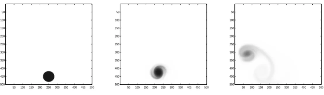
Figure 2: Concentration images extracted from a simulation of a shallow wa-ter model coupled with a concentration equation, images number 1 (left), 101 (middle), and 401 (right) respectively.
a concentration equation, from which a concentration image is extracted every 100 time steps. Figure 2 shows four such concentration images, corresponding
to the initial condition (first time step), and three intermediate states (10001st,
20001st and 40001st time steps respectively, corresponding to images number
101, 201 and 401 respectively).
3.2
Estimation of velocity fields between two images
Two consecutive images are extracted from these simulated data, see figure 3. We recall that one image is obtained from this model every 100 time steps, and hence there are 100 time steps (or 1 second) between these two images. We applied our algorithm to these two images, with the aim of identifying the entire
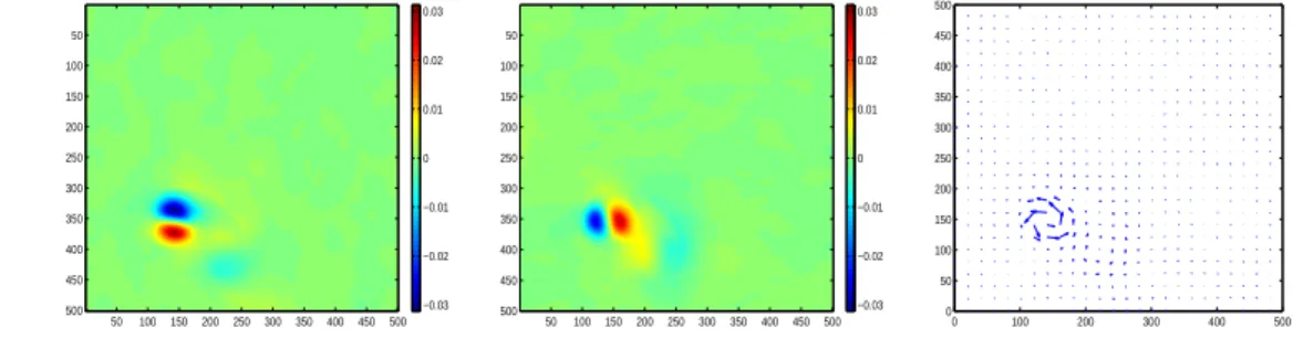
velocity field. The regularization norm is R1, defined by equation (5).
Figure 4 shows the longitudinal and transversal components of the identified velocity, and the corresponding velocity field. This result has been obtained without any multiscale approach, and without any a priori estimation of the velocity (i.e. the algorithm was initialized with u = 0 and v = 0). The structure of a vortex can be identified from these figures: the longitudinal component is negative on the top and positive on the bottom, and the transversal component is negative on the left and positive on the right side. This is the characteristic structure of a counterclockwise rotating vortex. Moreover, the mean of the
50 100 150 200 250 300 350 400 450 500 50 100 150 200 250 300 350 400 450 500 50 100 150 200 250 300 350 400 450 500 50 100 150 200 250 300 350 400 450 500
Figure 3: Concentration images I0 and I1 at time steps 25001 and 25101
re-spectively, corresponding to extracted images number 251 and 252 respectively.
50 100 150 200 250 300 350 400 450 500 50 100 150 200 250 300 350 400 450 500 −1.5 −1 −0.5 0 0.5 1 1.5 50 100 150 200 250 300 350 400 450 500 50 100 150 200 250 300 350 400 450 500 −1.5 −1 −0.5 0 0.5 1 1.5 50 100 150 200 250 300 350 400 450 500 50 100 150 200 250 300 350 400 450 500
Figure 4: Identified velocity between images I0 and I1: longitudinal (left) and
transversal (center) components, velocity field (right).
longitudinal component of the velocity is slightly negative and the mean of the transversal component is slightly positive. We have then identified a global displacement of the vortex to the top left of the domain.
50 100 150 200 250 300 350 400 450 500 50 100 150 200 250 300 350 400 450 500 −60 −40 −20 0 20 40 60 50 100 150 200 250 300 350 400 450 500 50 100 150 200 250 300 350 400 450 500 −60 −40 −20 0 20 40 60 0 5 10 15 20 400 600 800 1000 1200 1400 1600 1800 2000 2200
Figure 5: Difference between image I1and image I0transported by: a constant
null velocity field (initialization of the algorithm) (left), the identified velocity field after convergence of the algorithm (center) ; evolution of the cost function versus the number of iterations of the minimization process (right).
We can simply quantify the identification of the velocity field, by having
a look at the difference between the second image I1 and the first image I0
transported by the velocity. Figure 5 shows this difference at the beginning of the algorithm, when we initialize with a constant null velocity field, and at the end of the algorithm, with the identified field. It is clear that the first image has been well transported to the second one, and the reconstructed velocity field is reliable.
Figure 5 (right) shows the evolution of the first term of the cost function (see equation (3)) versus the iterations of the minimization process. Note that here only the difference between the two images (the first one being transported to the second one) is shown, not the regularization term. The algorithm con-verges in a few tens of iterations, and there is a sharp decrease in the very first iterations. This result proves the quality of the regularization and the efficiency of our algorithm, as one should keep in mind that we do not need any a priori estimation of the velocity field. The computation time is nearly 1 hour, as one iteration costs 3 minutes, with Matlab(R) on a 2.0 GHz laptop.
50 100 150 200 250 300 350 400 450 500 50 100 150 200 250 300 350 400 450 500 −0.03 −0.02 −0.01 0 0.01 0.02 0.03 50 100 150 200 250 300 350 400 450 500 50 100 150 200 250 300 350 400 450 500 −0.03 −0.02 −0.01 0 0.01 0.02 0.03 0 100 200 300 400 500 0 50 100 150 200 250 300 350 400 450 500
Figure 6: True velocity between images I0 and I1: longitudinal (left) and
transversal (center) components, velocity field (right).
Finally, these results are compared with the true velocity field, as the data are extracted from a known model trajectory. Figure 6 shows the true velocity components and field at time step 25001. It is difficult to compare this figure with figure 4. First, the scale is not the same in both figures, as one figure comes from the numerical model, showing a velocity in meters per second, and the other one shows an identified velocity in pixels per frame. As one pixel
corresponds to 6.10−3meter, and the time difference between two images is 100
time steps, i.e. 1 second, there is a 6.10−3 ratio between considering m.s−1
and pixel.f rame−1 velocities. For example, the maximum amplitude of the
identified velocity is 1.8 pixel per frame, i.e. 1.08 × 10⁻² m.s−1.
The global structure (vortex) of the velocity has been retrieved, but there is a difference between the identified velocity, that we should call apparent velocity, and the true velocity, both in shape (croissant shape instead of circular) and in amplitude (ratio ∼ 2). The difference (after rescaling from pixels to meters) between the apparent and true velocities comes from one main issue: the images are not acquired all the time, but every 100 time steps. Hence, in order to have a fair comparison, we should compute a global velocity field, corresponding to the displacement during 100 time steps, from the 100 instantaneous velocities
produced by the model, but this is an extremely difficult point. This global velocity is in some sense a Lagrangian integration during 100 time steps of the instantaneous velocity. This point should be addressed before considering the assimilation of such pseudo-observations, but the use of Lagrangian data assimilation schemes would probably help. Anyway, we have seen that the apparent velocity is very well identified, as the first image is well transported towards the second one.
In a more general framework, several other issues may increase the difference between apparent and true velocities. For example, there could be some vertical velocity, and the apparent velocity would be some two-dimensional projection of a three-dimensional evolution. In this case, as the data come from a synthetic two-dimensional experiment, we don’t have this problem. A second issue comes from the tracer transport modeling. Equation (14) does not reproduce quite well the transport phenomenon, but in this case, we also don’t have this problem, as the tracer concentration images are extracted from a trajectory of this equation. Finally, this difference is well known in wave propagation problems, as one can have a null apparent velocity while the true velocity is not equal to zero, and we refer to this domain for a more detailed comprehension of this problem (see e.g. [19]).
3.3
Choice of the regularization
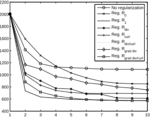
We now study the impact of the regularization norm on the results. We will consider the final value of the cost function as a criterion for the quality of the identified velocity field, as it measures exactly the difference between the second image and the first one transported to the second one. We are indeed interested in finding a velocity field that maps one image onto the second one, and the smaller the cost function is, the better the mapping is. We initialize all minimization processes with u = 0 and v = 0, and we consider 10 iterations.
1 2 3 4 5 6 7 8 9 10 400 600 800 1000 1200 1400 1600 1800 2000 2200 No regularization Reg. R0 Reg. R1 Reg. Rdiv Reg. Rcurl Reg. Rdiv/curl Reg. Rgrad div
Reg. Rgrad div/curl
Figure 7: Evolution of the cost function versus the number of iterations of the minimization process, for several regularizations.
Figure 7 shows the evolution of the cost function versus the number of iter-ations of the minimization process, for several regulariziter-ations. In order to make
an unbiased comparison, we recall that only the difference between the two
im-ages (image I1and image I0transported by the velocity field) is shown, not the
regularization part. We have compared the various regularizations introduced in section 2 (see equations (4 − 10) for the definition of the various norms).
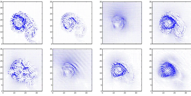
0 10 20 30 0 5 10 15 20 25 30 35 0 10 20 30 0 5 10 15 20 25 30 35 0 10 20 30 0 5 10 15 20 25 30 35 0 10 20 30 0 5 10 15 20 25 30 35 0 10 20 30 0 5 10 15 20 25 30 35 0 10 20 30 0 5 10 15 20 25 30 35 0 10 20 30 0 5 10 15 20 25 30 35 0 10 20 30 0 5 10 15 20 25 30 35
Figure 8: Zoom of the identified velocity fields between images I0and I1, using
various regularizations, namely from left to right and from top to bottom: no
regularization, R0, R1, Rdiv, Rcurl, Rdiv/curl, R∇div, R∇div/∇curl.
The first remark is that the R1 and Rdiv/curl regularizations produce the
same results, both for the cost function and the identified velocity field. This can be explained by the mathematical equivalence of these two norms, provided the velocity field has homogeneous boundary conditions (which is almost the case here). These two regularizations provide the best results, from all points of view: fastest decrease of the cost function, shape of the identified velocity, global structure of the velocity (translation to the top left, and counterclockwise rotating vortex).
Then, the R∇div/∇curl regularization has comparable results: the decrease
of the cost function is a little bit slower, but the final value is the same. The velocity field is a little more smooth, but this can easily be explained by the
equivalence of this norm with the L2norm of the Laplacian (still in the case of
homogeneous boundary conditions).
Some regularizations produce clearly bad fields, from a physical point of
view. For example, the Rcurl regularization has absolutely no interest, as the
velocity field cannot have a small curl. We can also see that the solutions
identi-fied with the R0or R∇div regularizations, or without any regularization, are not
very good, concerning both the decrease of the cost function and the identified
field. Finally, the most physical regularization is probably Rdiv, as we expect
cost function is not as good as some other regularizations, and the identified field has several false secondary recirculation vortices that are imposed by the transport constraint between the two images. Moreover, considering that the images are acquired every 100 time steps only, the velocity we want to identify between these two images is a time Lagrangian integration of many instanta-neous velocities, and it cannot have a divergence equal to zero (e.g. in the case of a perfect rotating vortex, by integrating many curl fields, one can obtain a curl-free field).
From the results presented in figures 7 and 8, we decide to consider only the
R1regularization in all the following experiments.
3.4
Multiscale approach
We present here a multiscale approach of our algorithm. We still initialize with u = 0 and v = 0, and we now look for a piecewise affine velocity field. We first work on a coarse grid, every 16 × 16 pixels, and identify a velocity field
between the two images I0and I1 which is piecewise affine every 16 × 16 pixels,
i.e. we minimize the cost function J (3) on the set C16 (see section 2.3). We
then provide this field as an initial guess to the minimization of the same cost
function on the set C8, in order to identify a 8 × 8 piecewise affine velocity field,
and so on. For each refinement of the mesh, we use the previous identified field (on a coarse grid) as an initial guess for the optimization process on the finer grid. At the end of the process, we obtain a field on the finest mesh, i.e. an estimation of the velocity at each pixel of the image. We use in the following
the regularization R1 defined by equation (5), as it provided the best quality
results and it is one of the simplest norms.
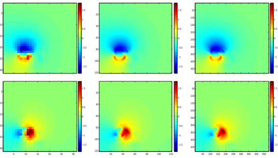
5 10 15 20 25 30 5 10 15 20 25 30 −1.5 −1 −0.5 0 0.5 1 1.5 20 40 60 80 100 120 20 40 60 80 100 120 −1.5 −1 −0.5 0 0.5 1 1.5 50 100 150 200 250 300 350 400 450 50 100 150 200 250 300 350 400 450 −1.5 −1 −0.5 0 0.5 1 1.5 5 10 15 20 25 30 5 10 15 20 25 30 −1.5 −1 −0.5 0 0.5 1 1.5 20 40 60 80 100 120 20 40 60 80 100 120 −1.5 −1 −0.5 0 0.5 1 1.5 50 100 150 200 250 300 350 400 450 50 100 150 200 250 300 350 400 450 −1.5 −1 −0.5 0 0.5 1 1.5
Figure 9: Identified velocity between images I0and I1in a multiscale approach:
longitudinal (top) and transversal (bottom) components of the velocity; 16 × 16 pixels, 4 × 4 pixels and 1 × 1 pixel piecewise affine respectively.
Figure 9 shows the identified fields, at every other refinement step, from a 16 × 16 pixels piecewise affine to a 1 × 1 pixel piecewise affine field. The multiscale approach works perfectly, as the identified solution on a coarse grid provides a very good estimation of the solution on a finer grid, and the 16 × 16 pixels piecewise affine field is already a good approximation of the final solution.
0 10 20 30 40 50 400 600 800 1000 1200 1400 1600 1800 2000 2200 1 2 3 4 5 6 7 8 9 400 600 800 1000 1200 1400 1600 1800 2000 2200
Figure 10: Left: evolution of the cost function versus the number of iterations of the minimization process, with a multiscale approach: one refinement every 10 iterations. Right: evolution of the cost function versus the number of iterations of the minimization process, with a multiscale approach: 5 iterations on the coarsest grid, and then one refinement every iteration.
Figure 10 (left) shows the evolution of the cost function versus the minimiza-tion iteraminimiza-tions in this multiscale approach. Recall that we have performed 10 iterations at every level of refinement. This clearly appears on figure 10 (left). Another interesting point is that the final solution is equivalent to the identified velocity field in the non multiscale approach, because the final value of the cost function is nearly equal to the final value in the non multiscale approach. The computation time of this multiscale minimization is nearly 1 hour, which is also equivalent to the previous approach.
We now consider a faster multiscale approach, in which we perform 5 itera-tions on the coarse grid (piecewise affine field every 16 × 16 pixels), and on finer grids the mesh is refined every iteration. This is motivated by figure 10 (left), which clearly shows that the minimization is mainly due to the first iteration after each refinement, and also by figure 9, which shows that the solution on the coarse grid is a very good approximation of the final solution. The final velocity identified by this faster multiscale approach does not differ much from the so-lution of the previous approach. This is confirmed by the final value of the cost function (569 instead of 568 in the previous multiscale approach), represented in figure 10 (right). Moreover, the computation time is now 6 minutes, which should be compared with the computation time of one iteration on the finest mesh (3 minutes). In the same time, without any multiscale approach, we would be able to perform only 2 minimization iterations, and the solution would not be so good: the cost function nearly equals to 740 in the non multiscale approach after 2 iterations. This fast multiscale approach is equivalent to 6 iterations of the non multiscale approach, and hence we have divided by 3 the computation time for the same results. Moreover, for some few images of this simulated
movie, the non multiscale approach was unable to converge towards a realistic solution, i.e. with a vortex located in this part of the image, using a constant (zero) velocity field as initial guess, whereas the multiscale approach has always provided the same kind of results. This is probably the most noticeable point of this approach.
For the further experiments, we will only consider this multiscale approach, as it provided nearly the best results, in a very short time.
3.5
Quality of the identified velocity
50 100 150 200 250 300 350 400 450 50 100 150 200 250 300 350 400 450 10 20 30 40 50 60 70 80 90
Figure 11: Quality estimate of the identified velocity, from 0 to 100% of relia-bility.
We now want to estimate the quality of the identified velocity. For this purpose, we use the quality estimate defined by equation (12). We applied the previously defined multiscale approach to the same two images, and the corresponding identified velocity is given in figure 9, on the right side. The quality estimate is represented in figure 11. Observe first that the two original images are equal on a large part of the domain, and hence the estimate is equal to zero almost everywhere, except in the vortex zone. This is due to the fact that any velocity field is able to transport one image to the other one in a region where they are constant and equal, and the quality of the identified field cannot be estimated. But in the vortex part, where the two images differ quite largely, the quality estimate has a large value, more than 90%, which confirms that the identified velocity is able to transport one image towards the second one in a very precise way.
As one application of velocity identification from images in geophysics is data assimilation, it is crucial to be able to provide with the observations some estimation of their quality, or their statistics of errors.
3.6
Object tracking
We now present an application of the 3D (2D in space + time) identification process. Assume that we have a particular object in the first image. In our case, we can identify one specific vortex. We can then limit the identification process to a region around this object. This region is propagated from one pair of images to the next one by the mean of the identified velocity. This allows to track this object in time.
50 100 150 200 250 300 350 400 450 500 50 100 150 200 250 300 350 400 450 500 50 100 150 200 250 300 350 400 450 500 50 100 150 200 250 300 350 400 450 500 50 100 150 200 250 300 350 400 450 500 50 100 150 200 250 300 350 400 450 500
Figure 12: Tracking of a specific region of the image: initial image (number 251) and region of interest in red (left); intermediate image (number 301) and propagated region of interest, using the identified velocity at each time step (middle); final image (number 351) and corresponding region of interest (right). Figure 12 shows the result of our tracking algorithm. We still consider the same starting image, in which we have defined a region of interest (represented by the red rectangle) of size 130 × 130. We have considered 100 successive images, from time step 25001 to 35001 (i.e. images number 251 and 351), and for each pair of consecutive images, we have identified a velocity field in the region of interest only, simply by applying our previous identification algorithm to the selected region instead of the entire image. Then, the red rectangle is propagated from one time step to the next one by the mean of the identified velocity. Figure 12 shows the tracking result after 50 and 100 images. The center of the vortex is still in the middle of the red box, even after 100 images, i.e. 10000 time steps of the numerical model. This result confirms that between two images, the apparent velocity is very well retrieved, and hence the displacement of the object is also well identified.
The time computation of this entire simulation (100 images) is less than 4 minutes. This is due to the drastic reduction of the problem size, as we identify the velocity in a small region of the image, and each velocity identification costs around 2 seconds.
However, in some experiments where the selected region is too small, the tracking is not so good, there can be a 10 to 20% difference between the the tracked region and the object of interest after 100 images. This is mainly due to a too small region, and the quality of the identified field is degraded, and also the mean of the identified field in this small region does not give a good estimation of the global displacement. The best way to track the object is to consider a reasonably large zone, e.g. not much smaller than in the example in figure 12.
4
Numerical results on experimental data
4.1
First experiment: colorant in water
We now consider data extracted from several experiments on the Coriolis ro-tating platform [7]. A large roro-tating turntable (diameter: 13 meters) allows to
reproduce the oceanic or atmospheric flows. Some colorant is inserted in the water as the platform rotates, and among the various measurement devices, a camera takes pictures of the experiment [13].
50 100 150 200 250 300 50 100 150 200 250 50 100 150 200 250 300 50 100 150 200 250
Figure 13: Concentration images I0 and I1 at time steps 5 and 6 respectively.
We consider two consecutive images extracted from these experimental data, see figure 13. The multiscale approach of our algorithm is used (see previous sections), looking first for a piecewise affine velocity field every 16 × 16 pixels, and then refining 4 times the mesh. The number of iterations is 50 on the coarse grid, and 1 on the finest grid. For each intermediate mesh, the minimization process is stopped when the decreasing rate of the cost function is lower than a threshold. 50 100 150 200 250 300 50 100 150 200 250 −8 −6 −4 −2 0 2 4 6 50 100 150 200 250 300 50 100 150 200 250 −5 0 5 10 15 0 5 10 15 20 25 0 5 10 15 20 25
Figure 14: Identified velocity between images I0and I1: longitudinal (left) and
transversal (center) components, velocity field (right).
Figure 14 shows the identified velocity components and field, using this mul-tiscale approach. The velocity field is represented every 12 pixels for visualiza-tion reasons. We have performed 50 iteravisualiza-tions on the coarse grid (16 × 16), then 5 on the 8 × 8 grid, 3 on the 4 × 4 grid, 1 on the 2 × 2 grid and 1 on the fine grid. The total computation time is less than 5 minutes. Note that, unlike the previous simulated experiments, the transversal and longitudinal components of the velocity do not have a zero (or nearly) mean. The first component has nearly −10 and 8 as extremal values, with a mean nearly equal to −2, whereas the second component has −7 and 21 as extremal values, with a mean nearly equal to 6. We recognize the characteristic shape of a vortex: if we subtract the
mean velocity, the longitudinal velocity is positive on the bottom and negative on the top of the domain, and the transversal velocity is positive on the right and negative on the left. Then, the global structure of the displacement is a rotating (counterclockwise) vortex in a translation field to the top (and a little bit left) of the domain.
0 10 20 30 40 50 60 0 0.5 1 1.5 2 2.5 3 3.5 4x 10 4
Figure 15: Evolution of the cost function versus the number of iterations of the minimization process, with a multiscale approach: 50 iterations on the coarsest grid, respectively 5, 3 and 1 iterations on the intermediate grids, and 1 iteration on the finest grid.
Figure 15 shows the evolution of the cost function versus the iterations. Here again, the crucial point is to perform a lot of iterations on the coarse grid, in order to identify the global structure of the velocity. Then, the refinement only gives details. This is why we have considered a large number of iterations on the coarse grid, and then very few iterations on the refined meshes. For a comparison, we tried with only 20 iterations on the coarse grid, and then twice more iterations on each refined mesh, and the final solution is worse (the final value of the cost function is higher) whereas the computation time is nearly twice larger.
In order to see the interest of the multiscale approach, we tried to identify directly the velocity on the finest grid, starting from a constant and null initial velocity field (i.e. without any a priori initial guess). Using the same computa-tion time as the multiscale approach, i.e. 5 minutes, we were able to perform only 3 iterations, and the final result is not satisfactory because the final value
of the cost function is 2.4 × 10⁴ (nearly what we get in less than 10 iterations
on the coarse grid, in the multiscale approach), and the identified velocity does clearly not show a rotating vortex. Even after 10 iterations, the identified field is far from being good, and the first image is not very well transported to the second one.
Finally, in order to visualize the quality of the reconstruction, figure 16
shows the difference between image I1and image I0transported by the velocity
field. On the left, we present the initial difference, using a constant and null velocity field. On the right, using the same scale, we have the final difference. The identified velocity transports very well the first image towards the second one. We can conclude that our identification algorithm of the apparent velocity works well on these experimental data.
Figure 17 shows the quality estimate of the identified velocity, from 0 (for unreliable data) to 100% (for a perfect identified velocity). The quality estimate
50 100 150 200 250 300 50 100 150 200 250 −600 −400 −200 0 200 400 600 50 100 150 200 250 300 50 100 150 200 250 −600 −400 −200 0 200 400 600
Figure 16: Difference between image I1and image I0transported by: a constant
null velocity field (initialization of the algorithm) on the left, the identified velocity field (after convergence of the algorithm) on the right.
50 100 150 200 250 300 50 100 150 200 250 10 20 30 40 50 60 70 80 90
Figure 17: Quality estimate of the identified velocity, from 0 to 100% of fiability, on the fine 1 × 1 grid.
is equal to 0 in most of the image. This is due to the lack of signal in both images (see figure 13). In the interesting part of the image, i.e. the vortex, there is some difference between the two original images, and hence the estimate can be computed. We can see that it is very high, globally larger than 90%. This was predictable from figure 16, in which we clearly see the good agreement between
the transported image I0and image I1.
We have also tried our algorithm on other images from the same experimental movie, with the same kind of results. We have also performed some simulations on another experimental movie, corresponding to the same kind of experiment (colorant inside water, on the same rotating platform, but different initial shape of the vortex), with the same kind of results also.
We should mention that on this experiment, we were able to compare qual-itatively our results with the PIV (particle imaging velocimetry) software used in the Coriolis platform [7]. The shape and global structure of the identified velocity fields is totally comparable, but the main disadvantage of PIV methods is to reduce drastically the resolution of the results, as it may produce 100 to 1000 times less vectors than pixels.
4.2
Second experiment: particles in water
We now consider a second experiment performed on the Coriolis rotating plat-form, in which some particles replace the colorant.
50 100 150 200 250 300 50 100 150 200 250 50 100 150 200 250 300 50 100 150 200 250
Figure 18: Concentration images I0and I1at time steps 28 and 29 respectively.
Figure 18 shows two images extracted from this other experimental movie. The structure of the velocity is the same as in the previous subsection: a vortex in a global translation displacement. We used the same multiscale approach as in the previous subsection, using a large number of iterations on the coarse grid, and then very few iterations on the refined grids, and finally only 1 iteration on the finest grid.
50 100 150 200 250 300 50 100 150 200 250 −6 −4 −2 0 2 4 6 50 100 150 200 250 300 50 100 150 200 250 −5 −4 −3 −2 −1 0 1 2 3 4 5 0 5 10 15 20 25 0 5 10 15 20 25
Figure 19: Identified velocity between images I0 and I1: longitudinal (top) and
transversal (bottom) components on the left, velocity field on the right. Figure 19 shows the identified velocity components and field, using this multiscale approach. The velocity field is represented every 12 pixels for vi-sualization reasons. The identified velocity is quite smooth, even though the regularization coefficient is the same as in the previous experimental results. Here again, it is very easy to see the global structure of the velocity field, with a characteristic counterclockwise rotating vortex, nearly located in the middle of the image. The global displacement of the structure is a small translation to the top, as the mean of the longitudinal components is nearly zero whereas the mean of the transversal component of the velocity is slightly positive.
Figure 20 shows the results of the identification process. On the left is represented the difference between the two original images, and on the right,
50 100 150 200 250 300 50 100 150 200 250 −600 −400 −200 0 200 400 600 50 100 150 200 250 300 50 100 150 200 250 −600 −400 −200 0 200 400 600
Figure 20: Difference between image I1and image I0transported by: a constant
null velocity field (initialization of the algorithm) on the left, the identified velocity field (after convergence of the algorithm) on the right.
the difference between the second image and the first one being transported by the identified velocity. Even if the original difference looks quite big, with a lot of small displacements everywhere, one can see that the smooth identified velocity provides a very good transport between these two images, as the difference has been drastically reduced.
0 5 10 15 20 25 30 0 0.5 1 1.5 2 2.5 3 3.5 4x 10 4
Figure 21: Evolution of the cost function versus the number of iterations of the minimization process, with a multiscale approach: 24 iterations on the coarsest grid, respectively 3, 2 and 2 iterations on the intermediate grids, and 1 iteration on the finest grid.
Figure 21 shows the evolution of the cost function during the minimization process. Once again, it appears clearly that the global decrease of the cost function is done on the coarse grid, and it seems extremely efficient and fast to first identify the global structure of the velocity on the coarse grid, and then refine for details. The total computation time of this experiment is 7 minutes.
We have compared the previous results with a non multiscale approach, on the same images, with the same numerical parameters. We have performed 10 iterations in the minimization process. We should recall that the identification process is done directly on the fine grid (1 × 1 pixel), and without any initial guess on the velocity field. Figure 22 shows the corresponding results. On the left are represented the two components of the identified velocity after 10 iterations, and on the right the quality of the transport between the two images.
50 100 150 200 250 300 50 100 150 200 250 −3 −2 −1 0 1 2 3 50 100 150 200 250 300 50 100 150 200 250 −2.5 −2 −1.5 −1 −0.5 0 0.5 1 1.5 2 2.5 50 100 150 200 250 300 50 100 150 200 250
Figure 22: Non multiscale approach for the identification of the velocity between
images I0 and I1: longitudinal (top) and transversal (bottom) components of
the velocity on the left, difference between image I1 and image I0 transported
by this field.
Several conclusions can be drawn from this figure. Firstly, the computation time of this experiment was 33 minutes, more than four times the computation time of the previous multiscale approach. Secondly, the quality of the identified field is not good, as can be seen in figure 22 on the right (this figure should be compared with figure 20 on the right). The right part of the vortex has not been well transported. Moreover, the convergence of the algorithm was achieved after these 10 iterations, and the final value of the cost function is more than 1.5 times the final value in the multiscale approach. All these remarks clearly demonstrate the interest of a multiscale approach, both for regularizing the problem, and for a fast and effective estimation of the velocity field.
50 100 150 200 250 300 50 100 150 200 250 10 20 30 40 50 60 70 80 90 10 20 30 40 50 60 70 80 10 20 30 40 50 60 70 10 20 30 40 50 60 70 80 90
Figure 23: Quality estimate of the identified velocity, from 0 to 100% of relia-bility, on the fine 1 × 1 grid (left) and on the 4 × 4 grid (right).
Figure 23 shows the quality estimate from equation (12) corresponding to the identified velocity, both on the fine grid (1 × 1 pixel) and on a coarser grid (4×4 pixels). The scale goes from 0 for a totally untrustable velocity to 100% for a fully reliable velocity. One should notice that outside the vortex, the quality is poor. This is due to the fact that there is more or less nothing in both images, and then there is no way to assess that we have identified the right velocity. For example, in the bottom right corner, both images have a signal equal to
0, and then any reasonable velocity can transport a zone of 0 to another one. On the contrary, in the vortex zone, the quality is much better, and is globally higher than 75%. This is due to the high signal in both images and also to the identification of an efficient transport field between the two images in this zone. We have previously seen in figure 20 that the quality of the identified velocity is very good in the high signal parts of the images, and this is confirmed with this estimate. The right part of figure 23 shows the same estimate on a coarser grid, and the corresponding estimate is a little bit smaller, because it is impossible to transport exactly a 4 × 4 pixels block to another one, and hence the difference
between image I1and transported image I0 is larger.
5
Conclusion
In this paper we presented an algorithm to estimate the motion between two images. This algorithm is based on the constant brightness assumption. A multiscale approach allows us to perform a minimization of the cost function in nested subspaces, the Jacobian matrix of the cost function being assembled rapidly at each scale using a finite element method. The coarse estimation allows one to avoid local minima, while the fine scales give more precise details.
Several regularization terms are discussed, and it appears that the L2 norm of
the gradient gives reliable results.
The results of this algorithm on simulated and real fluid flows are presented, and they are encouraging both from their computational efficiency and from the quality of the estimated motion.
As explained in the introduction, the extracted velocity fields can be seen as pseudo-observations of the velocity of the fluid, and the next step will be to consider the assimilation of these data. The results should be compared with the assimilation of classical data (e.g. sea surface heights in the case of oceanographic systems).
Acknowledgments
We greatly acknowledge the MOISE research project of INRIA Rhˆone-Alpes
(France) and the Coriolis project of LEGI (Grenoble, France) for providing us the synthetic and real data respectively. This work is partly done within the MOISE INRIA team and supported by the French National Research Agency (ANR ADDISA).
References
[1] R. Adrian. Particle imaging techniques for experimental fluid mechanics.
Ann. Rev. Fluid Mech., 23:261–304, 1991.
[2] L. Alvarez, C. Casta˜no, M. Garcia, K. Krissian, L. Mazorra, A. Salgado,
and J. Sanchez. A variational approach for 3d motion estimation of incom-pressible piv flows. pages 837–847, 2007.
[3] P. Ananden. A computational framework and an algorithm for the mea-surement of visual motion. Int. J. Comput. Vis., 2:283–310, 1989.
[4] S. Beauchemin and J. Barron. The computation of optical flow. ACM
Computing Surveys, 27(3):433–467, 1995.
[5] E. Blayo, S. Durbiano, P. A. Vidard, and F.-X. Le Dimet. Reduced order
strategies for variational data assimilation in oceanic models. Springer-Verlag, 2003.
[6] F. Bouttier and G. Kelly. Observing system experiments with the ecmwf data assimilation system. Quart. J. Roy. Meteor. Soc., 127:1469–1488, 2001.
[7] Coriolis rotating platform, website http://www.coriolis-legi.org/. [8] T. Corpetti, E. M´emin, and P. P´erez. Dense estimation of fluid flows. IEEE
Trans. Pattern Anal. Mach. Intel., 24:365–380, 2002.
[9] A. Cuzol, P. Hellier, and E. M´emin. A low dimensional fluid motion esti-mator. Int. J. Comput. Vis., 75:329–349, 2007.
[10] J. Fehrenbach and M. Masmoudi. A fast algorithm for image registration.
C. R. Acad. Sci. Paris, Ser. I, 346:593–598, 2008.
[11] J. M. Fitzpatrick. A method for calculating velocity in time dependent images based on the continuity equation. pages 78–81, San Francisco, USA, 1985. Proc. Conf. Comp. Vision Pattern Rec.
[12] J. M. Fitzpatrick. The existence of geometrical density-image transforma-tions corresponding to object motion. Comput. Vis. Grap. Imag. Proc., 44:155–174, 1988.
[13] J. B. Flor and I. Eames. Dynamics of monopolar vortices on the beta plane.
J. Fluid Mech., 456:353–376, 2002.
[14] GOES geostationnary satellite server http://www.goes.noaa.gov/. [15] B. Horn and B. Schunk. Determining optical flow. Artifical Intelligence,
17:185–203, 1981.
[16] E. Huot, T. Isambert, I. Herlin, J.-P. Berroir, and G. Korotaev. Data assimilation of satellite images within an oceanographic circulation model. Toulouse, France, 2006. Proc. Int. Conf. Acoustics Speech Sign. Proc. [17] T. Isambert, I. Herlin, and J.-P. Berroir. Fast and stable vector spline
method for fluid flow estimation. pages 505–508, San Antonio, USA, 2007. Proc. Int. Conf. Image Proc.
[18] R. Larsen, K. Conradsen, and B. K. Ersboll. Estimation of dense image flow fields in fluids. IEEE Trans. Geoscience Remote Sensing, 36(1):256–264, 1998.
[19] R. L. Lillie. Whole Earth Geophysics: an introduction textbook for
gelolo-gists and geophysicists. Prentice Hall, 1999.
[20] B. Lucas and T. Kanade. An iterative image registration technique with an application to stereo vision. pages 674–679, Vancouver, Canada, 1981. Proc Seventh International Joint Conference on Artificial Intelligence.
[21] J. Ma, A. Antoniadis, and F.-X. Le Dimet. Curvlets-based snake for multi-scale detection and tracking of geophysical fluids. IEEE Trans. Geoscience
Remote Sensing, 45(1):3626–3638, 2006.
[22] E. M´emin and P. Perez. Optical flow estimation and object-based segmen-tation with robust techniques. IEEE Trans. Image Proc., 7(5):703–719, 1998.
[23] Y. Michel and F. Bouttier. Automatic tracking of dry intrusions on satellite water vapour imagery and model output. Quart. J. Roy. Meteor. Soc., 132:2257–2276, 2006.
[24] P. Ruhnau, T. Kohlberger, C. Schn¨orr, and H. Nobach. Variational
opti-cal flow estimation for particle image velocimetry. Experiments in Fluids, 38(1):21–32, 2005.
Centre de recherche INRIA Bordeaux – Sud Ouest : Domaine Universitaire - 351, cours de la Libération - 33405 Talence Cedex Centre de recherche INRIA Lille – Nord Europe : Parc Scientifique de la Haute Borne - 40, avenue Halley - 59650 Villeneuve d’Ascq
Centre de recherche INRIA Nancy – Grand Est : LORIA, Technopôle de Nancy-Brabois - Campus scientifique 615, rue du Jardin Botanique - BP 101 - 54602 Villers-lès-Nancy Cedex
Centre de recherche INRIA Paris – Rocquencourt : Domaine de Voluceau - Rocquencourt - BP 105 - 78153 Le Chesnay Cedex Centre de recherche INRIA Rennes – Bretagne Atlantique : IRISA, Campus universitaire de Beaulieu - 35042 Rennes Cedex Centre de recherche INRIA Saclay – Île-de-France : Parc Orsay Université - ZAC des Vignes : 4, rue Jacques Monod - 91893 Orsay Cedex
Centre de recherche INRIA Sophia Antipolis – Méditerranée : 2004, route des Lucioles - BP 93 - 06902 Sophia Antipolis Cedex
Éditeur
INRIA - Domaine de Voluceau - Rocquencourt, BP 105 - 78153 Le Chesnay Cedex (France)