ISA -AN INVERSE SURFACE-BASED APPROACH FOR CORTICAL FMRI DATA PROJECTION

ISA - AN INVERSE SURFACE-BASED APPROACH FOR CORTICAL FMRI

DATA PROJECTION

Lucie Thiébaut Lonjaret

Christine Bakhous

Timothé Boutelier

Sylvain Takerkart

Olivier Coulon

?

_{Olea Medical, La Ciotat, France}

†

_{Aix-Marseille Univ., CNRS, Institut de Neurosciences de la Timone, Marseille, France}

_{Aix-Marseille Univ., CNRS, LSIS, Marseille, France}

ABSTRACT

Surface-based approaches have proven particularly rele-vant and reliable to study cortical functional magnetic re-sonance imaging (fMRI) data. However projecting fMRI volumes onto the cortical surface remains a challenging problem. Very few methods have been proposed to solve it and most of them rely on a simple interpolation. We propose here an original surface-based method based on a model representing the relationship between cortical activity and fMRI images, and a resolution through an inverse problem. This approach shows interesting pers-pectives for fMRI data processing as it is highly robust to noise and offers a good accuracy in terms of activations localization.

Index Terms— fMRI, surface-based method,

in-verse problem, signal reconstruction 1. INTRODUCTION

FMRI datasets are commonly analyzed in their ac-quisition space with volume-based methods. However, to hurdle the poor contrast to noise ratio (CNR) of fMRI data, these techniques usually apply a smoothing in the voxels space with very little consideration to the un-derlying brain anatomy, thus mixing informations that should not be (e.g. signals coming from opposite sides of a sulcus). Surface-based methods overcome this issue by studying the cortical signals in a domain approximating their original space : the cortical surface, hence keeping track of more relevant neighborhoods. Among those ap-proaches, two classes of techniques can be distinguished. The conceptually simplest ones rely on interpolation me-thods, such as the trilinear interpolation [1], to transpose the 3D data onto the cortical surface. The more sophis-ticated processes embed anatomically informed models. Those models are then fitted to the fMRI 3D data [2] or used to interpolate the 3D data onto the cortical surface [3, 4, 5]. Because the acquisition system is responsible for transposing the cortical blood oxygen level dependent

(BOLD) signal onto a cartesian voxel grid, we propose an Inverse Surface-based Approach (ISA) to reconstruct the cortical activity onto the cortical surface through solving the corresponding inverse problem. ISA requires several inputs : a cortical mesh of the white matter / grey mat-ter inmat-terface regismat-tered to the functional volumes, and the functional volumes corrected for head motion and slice timing. In this paper, we detail the construction of the forward model, introduce the corresponding inverse problem and present the methods to solve it. Several experiments are then conducted on both simulated and real datasets, that demonstrate the robustness of ISA to noise and its accuracy in terms of localization.

2. METHODS

2.1. From cortical activity to fMRI volume : for-ward model

The first step towards recovering the original cortical signal from MR images consists in defining the forward model (i.e. modeling how the acquisition process led the original cortical signals to the 3D images). This model should include both brain physiology and MR physics considerations, such as the shape of the BOLD signal, the partial volume effect (PVE), and the geometrical and architectural features of the cortex. We therefore started from the model exposed by Operto et al. [5]. This model suggests that signals IS on the cortical surface

(repre-sented by a mesh of Nn nodes) at node m result from

a weighted sum of the cortical activities a at neighbo-ring nodes n (Eq. 1), thus modeling the local induced activities by geodesic (i.e. following the cortical surface) weights ωgeo(see Fig. 1.b). It also supposes that the

si-gnals in the volume V (divided in Nv voxels) result from

a weighted sum of the local cortical signals on the sur-face (Eq. 1), thus modeling the PVE by weights ωnorm

Fig. 1. Normal (a) and geodesic (b) components of the model designed by Operto et al. [5].

surface (see Fig. 1.a). (

IS(m) =PN_n=1n ωgeo(m, n)a(n)

V (v) =PNn

m=1ωnorm(v, m)IS(m)

(1)

However this model suffers from some drawbacks. First, the cortical mesh often has a variable density, which re-sults in each node representing portions of the cortical surface of various size. As the cortical mesh is a discreti-zed version of a continuous surface, the cortical activity

a at a given node n stands actually for all the cortical

activities γ(i) contained by the Voronoï cell Cn

associa-ted to n. Because we have no prior on the distribution of those activities within Cn, we consider γmean(n) the

average activity over Cn and obtain Eq. 2.

a(n) = area(Cn)γmean(n) (2)

Combining those considerations with Eq. 1 leads to Eq. 3, thus taking into account the mesh variable density.

(

V (v) =PNn

n=1M (v, n)γmean(n)

M (v, n) =PNn

m=1ωnorm(v, m)ωgeo(m, n)area(Cn)

(3) Second, we generalize Eq. 3 to time-series of volumes by simple concatenation (Eq. 4) to process simultaneously all the fMRI volumes of one session. Hence the forward model M links real cortical signals Γ and fMRI volumes

V . Each column of V represents the fMRI volumetric

data at time t. Each column of Γ similarly stands for the signals on the cortical mesh nodes γmean at time t.

V = M Γ (4)

2.2. From volume to surface : inverse problem We solve the corresponding inverse problem, which consists in inverting the forward model (Eq. 4), with the method of regularized least-squares. The number of mesh nodes often exceeding by far the number of relevant func-tional voxels, our problem is highly underdetermined and thus ill-posed and ill-conditioned. Therefore we optimize a cost function composed of three terms, including two terms of regularization. The first term fd(Eq. 5) reflects

how close the fMRI volumes predicted eV from the

for-ward model are to the observed data V . The noise cova-riance matrix R, estimated with [6], balances this term.

fd(eΓ) =

T r((V − M eΓ)tR−1(V − M eΓ))

2 (5)

To begin with, the cortical signal does diffuse locally [7]. This prior of smoothness can be modeled by a spa-tial regularization term fs(Eq. 6) relying on the geodesic

distance between neighboring nodes. Here we introduce cliques notations. A clique ciis defined by a pair of

corti-cal mesh nodes (ni,1, ni,2) and a weight which depends on

the geodesic distance dgbetween those two nodes and on

a normalization term Dnorm. Such a normalization term,

based on the number Ω(n) of neighboring nodes of each of the two nodes of ci, is necessary to cope with the mesh

irregularity and ensure the same power of regularization at each mesh node.

           fs(eΓ) = T r(eΓtDtDeΓ) Di,j = δ_j,ni,1−δ_j,ni,2

dg(ni,1,ni,2)Dnorm(ni,1,ni,2) with δj,l=

(

1 if j = l 0 else

Dnorm(ni,1, ni,2) =

q _{Ω(ni,1)Ω(ni,2)}

Ω(ni,1)+Ω(ni,2)

(6) Furthermore, BOLD signals measured with fMRI come from the hemodynamic response function (HRF) which is smooth in time. Therefore, we define a tempo-ral regularization term ft (Eq.7) with T expressing the

second order differential.

ft(eΓ) = T r(eΓTtT eΓt) (7)

2.3. Optimization

The regularized least square estimator reaches the solution by minimizing the corresponding cost function where λD and λT are respectively the spatial and

tem-poral regularization coefficients :

f (eΓ) = fd(eΓ) + λDfs(eΓ) + λTft(eΓ) (8)

Minimizing this cost function amounts to nullifying its gradient, thus resulting in the following Sylvester equa-tion (see [8] for more informaequa-tion on such equaequa-tions) :

H eΓ + eΓG = K with      H = Mt_R−1_{M + 2λ} DDtD G = 2λTTtT K = MtR−1V (9) Because operator H is positive definite by construction and operator G is semi-positive definite, we chose to use the linear conjugate gradients (CG) algorithm [9]. Indeed, this optimization technique is guaranteed to converge, under the previously mentioned conditions, to

the unique solution, accurately and in a short amount of time.

Regularization coefficients were set as follows. In or-der to ensure the best spatial conditioning of the problem and guarantee an optimal convergence of the CG, λDwas

chosen as to minimize the condition number (i.e. the ratio of the largest over the smallest eigenvalues) of operator

H (Eq. 9). Hence λD becomes directly dependent of the

mesh geometry and resolution.The optimal λT was set

empirically using an independent set of simulated data with meshes of various resolution. We found that the op-timal λT was quite stable across mesh resolutions and

we set it at the empirical value of λT = 15.

3. RESULTS 3.1. Experiments

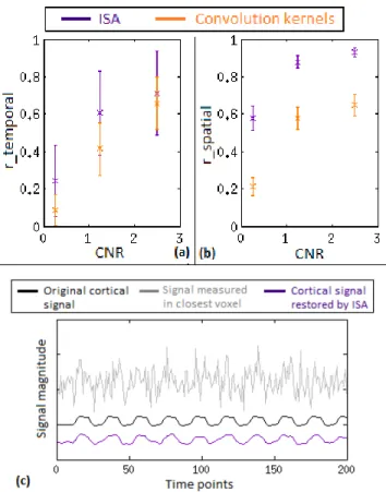
ISA’s performances were assessed on both simulated fMRI data, and real data. Simulated data were genera-ted according to the following process. First, a cortical mesh was extracted from real data. Then we simulated a smooth activation blob of 1cm of radius on this mesh, thus generating a surface map. Thereafter we construc-ted a block paradigm, using 10 repetitions of this map for the ”off” blocks and multiplying these blocks by the desi-red percent of signal change (here PSC = 5) plus 1. Once the paradigm built, each node signal was convolved with SPM (http ://www.fil.ion.ucl.ac.uk/spm/) HRF model (considering a TR of 2s), thus producing a time-series of maps representing the BOLD fluctuations in time (Fig. 2.c - black). Finally, the forward model (Eq. 4) was ap-plied to generate the corresponding fMRI volumes. Va-riable levels of Gaussian noise were added (Fig. 2.c - light grey) to get realistic fMRI data with variable CNR (i.e. the ratio of the highest temporal variations amplitude over the noise standard deviation). We conducted a noise robustness experiment on simulated fMRI volumes cor-responding to 50 different realizations of activation blobs spread across the cortical surface for 3 levels of Gaussian noise (CNR = 2.5, 1.25 and 0.25). Finally, we produced a qualitative analysis of the spatial aspect of the projection using real data from a voice localizer experiment [10] : vo-lumetric t-maps estimated using SPM, for the contrast ‘voice - non voice’, showing the individual location of the temporal voice areas, were projected on the cortical surface for four subjects. Results of all experiments were compared with those produced using the convolution ker-nels method that was shown to outperform all other me-thods [5]. These experiments used cortical meshes pro-duced by the BrainVisa software (http ://brainvisa.info), with an average number of 60,000 nodes. Functional data had a spatial resolution of 3x3x3mm3_.

Fig. 2. Results of the robustness to noise assessment. Average and standard deviation of rtemporal (a) and

rspatial(b) over 50 realization. Qualitative representation

of temporal activity at the center node of an activation blob (c).

3.2. Robustness to noise

Projection of time series was performed on all simu-lated datasets using ISA and the convolution kernels me-thod. We evaluated the quality of the reconstructed si-gnal in the spatial and temporal domains by computing the spatial Pearson correlation (rspatial) with the

origi-nal spatial map before application of the forward model, and the temporal Pearson correlation (rtemporal) with

the original paradigm. For rtemporal we considered only

the temporal signals of the nodes localized within the ac-tivation area, whereas we considered the whole cortical surface for rspatial. Under noisy conditions ISA

outper-forms the convolution kernels both in terms of localiza-tion and correlalocaliza-tion to the experimental paradigm (Fig. 2.a,b). Indeed, we observe that ISA restores high values of rtemporaleven with poor CNR, and only starts to face

real difficulties when the CNR goes below 1, that is to say when the fMRI signal contains more noise than va-riations of interest. Furthermore rspatial is clearly higher

for ISA than for the convolution kernels, showing a bet-ter control of the spatial regularization. It is important

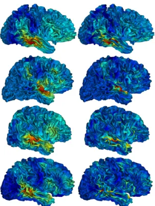
Fig. 3. Results of the convolution kernels (left) and ISA (right) applied on real data (colorscale is subject de-pendent).

to note that the spatial regularization term is set to opti-mize the spatial conditioning of the problem, but at the cost of a loss in signal magnitude restoration (Fig. 2.c). 3.3. Real data

Comparing the effect of ISA and the convolution ker-nels method, shown in Fig. 3, we noticed that there is an overall similarity of the activation patterns, but im-portant local differences can be observed. In particular, it is clearly visible that peaks of activation are more fo-cal with ISA. This shows a deconvolution effect that is intrinsic to the inverse problem approach : on top of ISA offering a more controlled spatial regularization, the for-ward model embeds several sources of signal mixing and the inverse resolution disentangle them. This could lead to a better spatial accuracy for functional data analysis.

4. CONCLUSION AND FUTURE WORK We presented here a new surface-based approach to project fMRI data onto the cortical surface. This tech-nique is highly flexible and offers a general framework where it is easy to introduce other prior knowledges as long as they can be expressed as a function. Moreover

ISA offers a good spatial and temporal accuracy even when faced to really noisy data. Future work will include experiments to assess ISA robustness to other kinds of errors arising from the preprocessing pipeline, such as anatomy-function registration errors or surface segmen-tation errors, and applications to real datasets.

5. ACKNOWLEDGMENT

We thank P. Belin for providing the ‘temporal voice area’ datasets.

6. REFERENCES

[1] A. Andrade, F. Kherif, J. Mangin, K. Worsley, A. Paradis, O. Simon, S. Dehaene, D. Le Bihan, and J. B. Poline, “Detection of fmri activation using cor-tical surface mapping,” Human Brain Mapping, vol. 12(2), pp. 79–93, 2001.

[2] S. J. Kiebel, R. Goebel, and K. J. Friston, “Anato-mically informed basis functions,” Neuroimage, vol. 11, pp. 656–667, 2000.

[3] J. Warnking, M. Dojat, A. Guérin-Dugué, C. Delon-Martin, S. Olympieff, N. Richard, A. Chéhikian, and C. Segebarth, “fmri retinotopic mapping–step by step,” Neuroimage, vol. 17(4), pp. 1665–1683, 2002. [4] C. Grova, S. Makni, G. Flandin, P. Ciuciu, J. Got-man, and J. B. Poline, “Anatomically informed in-terpolation of fmri data on the cortical surface,”

Neuroimage, vol. 31(4), pp. 1475–1486, 2006.

[5] G. Operto, R. Bulot, J. L. Anton, and O. Coulon, “Projection of fmri data onto the cortical surface using anatomically-informed convolution kernels,”

Neuroimage, vol. 39(1), pp. 127–135, 2008.

[6] John Immerkaer, “Fast noise variance estimation,”

Computer vision and image understanding, vol. 64,

no. 2, pp. 300–302, 1996.

[7] P. B. Johnson, S. Ferraina, and R. Caminiti, “Cor-tical networks for visual reaching,” Experimental

Brain Research, vol. 97(2), pp. 361–365, 1993.

[8] J. D. Gardiner, A. J. Laub, J. J. Amato, and C. B. Moler, “Solution of the sylvester matrix equation axb t+ cxd t= e,” ACM Transactions on

Mathe-matical Software (TOMS), vol. 18(2), pp. 223–231,

1992.

[9] S. Karimi, “Global conjugate gradient method for solving large general sylvester matrix equation,”

Journal of Mathematical Modeling, vol. 1, pp. 15–

27, 2013.

[10] P. Belin, R. J. Zatorre, P. Lafaille, P. Ahad, and B. Pike, “Voice-selective areas in human auditory cortex,” Nature, vol. 403(6767), pp. 309–312, 2000.