HAL Id: hal-01809627
https://hal.archives-ouvertes.fr/hal-01809627v2
Submitted on 4 Dec 2019
HAL is a multi-disciplinary open access
archive for the deposit and dissemination of
sci-entific research documents, whether they are
pub-lished or not. The documents may come from
teaching and research institutions in France or
abroad, or from public or private research centers.
L’archive ouverte pluridisciplinaire HAL, est
destinée au dépôt et à la diffusion de documents
scientifiques de niveau recherche, publiés ou non,
émanant des établissements d’enseignement et de
recherche français ou étrangers, des laboratoires
publics ou privés.
Building an effective and efficient background knowledge
resource to enhance ontology matching
Amina Annane, Zohra Bellahsene, Faical Azouaou, Clement Jonquet
To cite this version:
Amina Annane, Zohra Bellahsene, Faical Azouaou, Clement Jonquet. Building an effective and
ef-ficient background knowledge resource to enhance ontology matching. Journal of Web Semantics,
Elsevier, 2018, 51, pp.51-68. �10.1016/j.websem.2018.04.001�. �hal-01809627v2�
Building an effective and efficient background knowledge resource to enhance
ontology matching
Amina Annane1,2, Zohra Bellahsene2, Fai¸cal Azouaou1, Clement Jonquet2,3
1Ecole nationale Sup´erieure d’Informatique, BP 68M, 16309, Oued-Smar, Alger, Alg´erie 2LIRMM, Universit´e de Montpellier, CNRS, Montpellier, France
3Center for BioMedical Informatics Research (BMIR), Stanford University, USA
Abstract
Ontology matching is critical for data integration and interoperability. Original ontology matching approaches relied solely on the content of the ontologies to align. However, these approaches are less effective when equivalent concepts have dissimilar labels and are structured with different modeling views. To overcome this semantic heterogeneity, the community has turned to the use of external background knowledge resources. Several methods have been proposed to select ontologies, other than the ones to align, as background knowledge to enhance a given ontology-matching task. However, these methods return a set of complete ontologies, while, in most cases, only fragments of the returned ontologies are effective for discovering new mappings. In this article, we propose an approach to select and build a background knowledge resource with just the right concepts chosen from a set of ontologies, which improves efficiency without loss of effectiveness. The use of background knowledge in ontology matching is a double-edged sword: while it may increase recall (i.e., retrieve more correct mappings), it may lower precision (i.e., produce more incorrect mappings). Therefore, we propose two methods to select the most relevant mappings from the candidate ones: (1) a selection based on a set of rules and (2) a selection based on supervised machine learning. Our experiments, conducted on two Ontology Alignment Evaluation Initiative (OAEI) datasets, confirm the effectiveness and efficiency of our approach. Moreover, the F-measure values obtained with our approach are very competitive to those of the state-of-the-art matchers exploiting background knowledge resources.
Keywords: Ontology matching, Ontology alignment, Background knowledge, Indirect matching, External resource, Anchoring, Derivation, Background knowledge selection, Supervised machine learning.
1. Introduction
Ontologies provide conceptual models to represent and share knowledge. Some of the data management challenges for which ontologies are often used include interoperabil-ity [55] and data integration [35]. In recent years, because of the large number of ontologies developed, especially in domains that produce and manage an increasing amount of data (such as biomedicine [43]), these challenges have become increasingly complex. To achieve interoperabil-ity and integration, one solution is to identify mappings (correspondences) between different ontologies of the same domain. This process is known as ontology matching or ontology alignment.
Ontologies are heterogeneous because they have been designed independently, by different developers, and fol-lowing diverse modeling principles and patterns. This het-erogeneity makes the matching process complex [20]. The
first ontology matching methods were based only on the lexical and structural content of the ontologies to align; this is known as direct matching or content-based match-ing. To that end, many syntactic and structural similarity measures have been developed [8, 42, 20]. However, direct matching is less effective to find correspondences between concepts that are equivalent, but described with dissimilar labels and structured with different modeling views [1, 50]. To overcome this semantic heterogeneity, the commu-nity has turned to the exploitation of external knowledge resource(s), commonly called background knowledge re-sources. In contrast to direct matching, this approach is known as indirect matching, BK-based matching or context-based matching [37], as it exploits external resources to identify mappings between the ontologies to align.
The BK-based matching approach raises two main is-sues: (i) how to select (or build) background knowledge re-source(s) for a given ontology matching task? and (ii) how to concretely use the selected background knowledge re-source(s) to enhance the quality of the matching result?
In the literature, several works have addressed these
Email addresses: [email protected] (Amina Annane1,2),
[email protected] (Zohra Bellahsene2), [email protected] (Fai¸cal Azouaou1), [email protected] (Clement Jonquet2,3)
two issues jointly or separately. The selection of back-ground knowledge resources consists in choosing m re-sources among the n possible ones [23, 27, 9, 37]. Although only fragments of the m resources may actually prove ef-fective for discovering new mappings, entire resources are selected. In addition, almost all previous works exploit the selected resources independently of each other [46, 25], whereas, as we will show in this paper, more correct map-pings may be identified when we combine the selected re-sources into a single one.
In this article, we propose a novel approach to build a customized background knowledge resource from a set of ontologies to derive equivalence mappings. This approach is inspired from our previous work [3]. The built resource reduces the computation-time cost of the BK-based match-ing approach (i.e., efficient), and allows to improve the quality of the alignments generated by the direct match-ing (i.e., effective).
In [3], we considered the mappings stored in the NCBO BioPortal repository as background knowledge [43]. How-ever, we cannot find such mapping repository in every do-main. Therefore, in this article, we tried to make our approach more generic taking a set of ontologies as input and using an automatic matcher to extract the mappings to be used as background knowledge.
The use of external knowledge resources in ontology matching is a double-edged sword. Indeed, though these resources provide new information to find correct map-pings, incorrect mappings may also be generated [37]. Con-sequently, selecting correct mappings from the candidate ones is particularly challenging in the context of BK-based matching. In this article, we propose two new selection methods. The first one is based on a set of rules, while the second one is based on the supervised machine learn-ing technique. To enable the use of a classification machine learning algorithm, we designed a set of 27 attributes based on the built background knowledge resource.
We performed extensive experiments on two datasets taken from OAEI1, with two sets of preselected
ontolo-gies, to evaluate the performance of our approach. The experiment results confirm the efficiency and effectiveness of our approach. Moreover, we compared our results to those of the state-of-the-art systems that exploit back-ground knowledge resources. Our F-measure values are very competitive relative to the best ones reported in the literature.
To sum up, the main contributions of this article are: • A formalized general workflow for BK-based
ontol-ogy matching;
• A novel and dynamic approach to building a back-ground knowledge resource from a set of ontologies; • A BK-based matching approach that uses the built
background knowledge resource;
1http://oaei.ontologymatching.org/
• Two final mapping selection methods: a rule-based method, and a machine-learning based one.
• Extensive experiments on two OAEI datasets to demon-strate the efficiency of the built background knowl-edge resource, and the effectiveness of our approach. The remainder of this paper is organized as follows. In Section 2, we define the basic notions used herein and pro-vide a brief overview of our approach. We then describe the three main steps of our approach in detail. In Sec-tion 3, we review the selecSec-tion and building of the back-ground knowledge resource. In Section 4, we show how the built resource is used to derive candidate mappings. In Section 5, we describe our methods for selecting final mappings. In Section 6, we discuss the efficiency of our approach. In Section 7, we present the experimental ma-terial used for the evaluation. In Section 8, we present our results for OAEI Anatomy and LargeBio datasets. In Section 9, we discuss some limitations of our work. In Sec-tion 10, we provide a summary of related work. Finally, in Section 11, we conclude and discuss some future research.
2. Preliminaries
In this section, we define the various concepts under-lying our approach.
2.1. Ontology matching
Ontology matching can be formally defined as a function that takes two ontologies Os and Ot, a set of
parameters P , and a set of resources R, and returns an alignment A between Osand Ot.
An Alignment of ontologies Osand Otis a set of
map-pings between their different entities es and et.
A Mapping (or a correspondence) between an entity es(e.g., property, class) belonging to ontology Osand an
entity et belonging to ontology Ot is a four-tuple of the
form: m = hes, et, r, ki where:
• r is a relation such as equivalence (≡), more general (w), less general (v), etc.
• k is a confidence score (typically in the [0, 1] range) holding for the correspondence between the entities es and et.
A Similarity measure is a function f : Es× Et →
[0..1] where Es is the set of Os entities and Et is the set
of Otentities. For each pair of entities (es, et), a
similar-ity measure computes a real number, generally between 0 and 1, expressing the similarity between the two entities. There are several kinds of similarity measures: syntactic, semantic and structural [8, 44, 42].
A Matcher is a matching algorithm that implements one similarity measure or combines several to discover map-pings between ontologies. The term Matcher is also used in the literature to identify an ontology matching system [15]. 2.2. Ontology matching evaluation
Evaluating a given alignment is usually done with three measures: precision, recall and F-measure [11]. These measures are computed with respect to a reference align-ment that contains all the correct mappings. Precision is defined as the number of correctly identified mappings di-vided by the total number of mappings found (correct + incorrect). Recall is defined as the number of correctly identified mappings divided by the number of all possi-ble correct mappings (the size of the reference alignment). A perfect precision score of 1.0 means that every mapping returned by the matcher is correct; Precision measures cor-rectness. A perfect recall score of 1.0 means that all correct mappings were returned; Recall measures completeness. The F-measure is the harmonic mean of precision and re-call. It measures the overall accuracy of an alignment. Let A be an alignment produced by a given matcher and R the reference alignment. Precision, Recall and F-measure are computed as follows:
P recision = |A∩R||A| Recall = |A∩R||R|
F − measure = 2∗P recision∗Recall P recision+Recall
2.3. Background knowledge
In the context of ontology matching, there is no com-monly accepted or strict definition of what background knowledge is. We define it as any set of external knowl-edge resources that provides lexical or semantic informa-tion about the domain(s) of the ontologies to align or some of the entities therein. It could be any datasets related to the ontologies to align, other ontologies than the ones to align, other previously generated mappings, lexical re-sources, the Web, etc.
In this article, we use the acronym BK to refer to a background knowledge resource used within the matching process. For instance, if such a resource is an ontology, we will call it a BK ontology. Similarly, the expression BK-based method denotes a method that exploits a background knowledge resource.
2.4. Supervised machine learning
Supervised machine learning is the task of automat-ically inferring a function from training data [40]. The learned function f : x → y maps the input object x to an output y. When using the machine learning technique for a classification task, the learned function is called a classifier. The input x is composed of a set of attribute
values that describe the object to classify, while the out-put y is the class in which the object x will be classified by the learned classifier. The training data is a set of objects already classified (containing both attributes and class), while the test data is the set of objects to classify. A su-pervised machine learning algorithm analyzes the training data and produces a classifier that will be used to classify the test data objects.
2.5. Overview of our approach
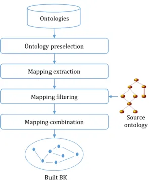
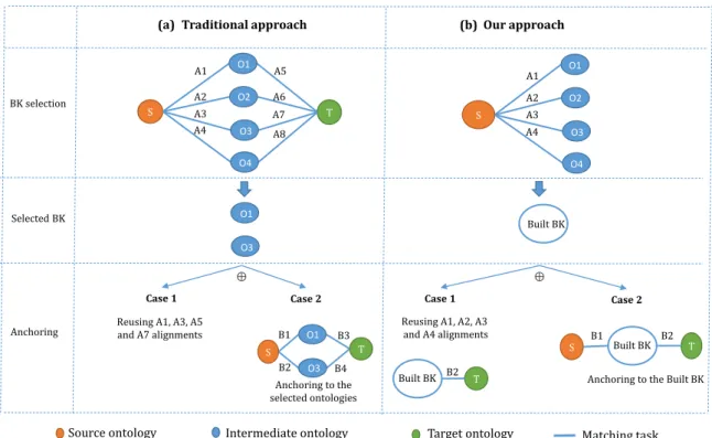
As shown in Figure 1, the general workflow of our BK-based matching approach includes three main steps. The first step consists in selecting a BK from an initial set of ontologies. In our approach, we do not select complete on-tologies; instead we select concepts from the initial ontolo-gies. We then combine the selected concepts in one single resource that we call the built BK. In the second step, we exploit the built BK to generate all possible candidate mappings between the ontologies to align. The last step consists in selecting the most relevant candidate mappings to produce the final alignment.
BK Selection BK Use Final mapping selection
Figure 1: Main steps of our BK-based ontology matching approach.
3. BK Selection
We can formally define BK selection as a function that takes a set of knowledge resources KR, a set of ontologies to align O, and optionally, a set of parameters P (e.g., threshold values), and returns the BK that will be used in the matching process. The returned BK may be a subset of KR [23], or a novel resource built from KR (our approach). For ontology matching, the automatic selection of on-tologies as background knowledge has been proposed in several works [50, 46, 27, 23]. However, all these methods return complete ontologies as a final BK for the matching process. Our hypothesis is that within each BK ontology, especially large ones, only fragments may actually prove effective. Hence, the issue is that of the selection of these fragments from each BK ontology and their combination to build an effective and efficient BK. In our approach, we tackle this issue by selecting only the relevant concepts from the initial ontologies related to the matching task. We then combine these selected concepts to build the BK. As we will experimentally demonstrate, the built BK has a reduced size comparing to the preselected ontologies size, which improves the efficiency of the BK-based matching without loss of effectiveness. Furthermore, the built BK in-terconnects concepts from different preselected ontologies via mappings, thereby generating mappings across several intermediate ontologies.
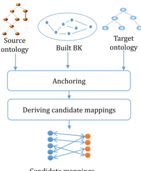
In the following, we detail the four steps involved in the BK selection process (see Figure 2).
Mapping extraction Mapping combination Built BK Mapping filtering Source ontology Ontology preselection Ontologies
Figure 2: Overview of the BK selection process.
3.1. Ontology preselection
Today, a simple Google Search for ”filetype:owl” re-turns around 34K results. Fittingly, these ontologies are often organized per domain or community in ontology li-braries [56, 10] such as the NCBO BioPortal, the AgroPor-tal [33] or the Marine Metadata Interoperability repository [49]. Ontology preselection consists in determining which ontologies to consider for the BK selection process among all the ontologies that exist. It aims at reducing the search space for the BK selection process by eliminating at the outset ontologies that would not be effective to identify new mappings (e.g., ontologies that are not of the same domain as the ontologies to align). The preselected on-tologies may be an ontology repository [9], a specific set of ontologies [23, 22, 27] or all ontologies indexed by a given semantic web search engine [50, 37].
In the related works, ontology preselection has not been formalized as a step of the BK-based ontology matching workflow, except in [37] where ontology preselection was called ontology arrangement.
In this article, we do not focus on automating ontology preselection. In our approach, and, at the best of our knowledge, in all related works, ontology preselection is performed manually [50, 23, 22, 27, 37].
3.2. Mapping extraction
The experiments reported in [29, 50, 37] showed that combining several BK ontologies generates more correct mappings. Figure 3 illustrates this benefit, sampled from our evaluation. Each concept is represented with the term: ontology#ConceptIdentifier and interconnected with map-pings. The source and target concepts are linked via at least two intermediate concepts which belong to two differ-ent BK ontologies. Such correct mapping would not have
been identified if we had used each intermediate ontology separately from the others (one intermediate concept at a time). Therefore, in this step, we extract all possible mappings between the preselected ontologies to be able to generate mappings across several intermediate ontologies.
NCI#External-ear-infection
GALEN#OtitisExterna RCTV2#F502z00
DOID#9463
SNOMED#Otitis-externa-NOS
Figure 3: Example of a correct mapping between NCI and SNOMED derived across intermediate concepts from different BK ontologies.
Let S = {O1, O2, ..., On} be the set of preselected
on-tologies. In this step, each ontology Oi in S is matched
to the other preselected ontologies that have a higher in-dex (i.e., Oi+1, Oi+2,....,On). The matching of each
cou-ple of ontologies (Oi, Oj) provides an alignment that is
a set of s mappings Aij = {m1, m2, ..., ms}. For n
pre-selected ontologies, the result is the union of
n−1
P
i=1
(n − i) alignments. More specifically, the result is the union of all mappings that compose the different alignments Aij:
M =Sn−1
i=1
Sn
j=i+1Aij.
The easiest way to extract these mappings is to use an automatic matcher. Several state-of-the-art matchers, such as YAM++ [41], LogMap [30], AML [24], etc., are readily available. As shown in previous OAEI campaigns, these systems provide high-quality alignments (i.e., align-ments with high F-measure score). Furthermore, if avail-able, mappings between the preselected ontologies that are manually created or human-curated should be added to the automatically extracted ones. For instance, in the biomed-ical domain, cross-references between OBO Foundry on-tologies [52] may be considered as manual mappings. Note that the mapping extraction task may be ignored if the preselected ontologies are not to be combined.
3.3. Mapping filtering
The preselected ontology concepts likely to generate new mappings should be related directly or indirectly to the source ontology. Conversely, those concepts not re-lated to the source ontology will not help generate new mappings. Hence, it seems more efficient to eliminate the latter at the outset.
We start by matching the source ontology Os to the
preselected ontologies in S. In order to improve efficiency, the smallest of the ontologies to align is chosen as the source ontology. The mappings obtained by matching the source ontology to the preselected ontologies initialize the set of filtered mappings, noted F M . Recursively, we enrich F M by selecting all the mappings in M related to the target concepts of mappings already present in F M , and so on, until no new mapping is found in M . More precisely, until all mappings related to the source ontology in M are in F M . In each step, F M is enriched as follows:
F M = F M ∪ {mi/mi ∈ M and Cs(mi) = Ct(mj) and
mj∈ F M }
where Cs(mi) is a function that returns the source
con-cept of the mapping mi and Ct(mj) is a function that
returns the target concept of the mapping mj.
3.4. Mapping combination
Mappings filtered in the previous step are then com-bined in one unique graph where nodes are concepts and edges are mappings that link these concepts. This combi-nation insures that each concept appears only once (i.e., mappings that share a concept are merged). Figure 4 shows an example of mapping combination. m1 and m2
are two mappings that have a common concept e2. The
combination keeps only one occurrence of the concept e2.
Note that, thanks to this combination, concepts that are not directly connected (e1 and e3 in Figure 4) may be
in-directly connected through common concepts. m1= m2= e2 e1 e2 e3 Combination e1 e2 e3 ≡ ≡ ≡ ≡
Figure 4: Mapping combination example.
In the resulting graph, each selected concept (node) is described with four attributes: (i) the URI of the concept, (ii) the URI of the ontology to which the concept belongs, (iii) the preferred label of the concept and (iv) the concept synonyms. The mappings (or edges) between concepts are described with three attributes: (i) the source from which each mapping has been extracted. It may be the name of a resource such as UMLS, or the ontology matching tool name when the mapping was generated automatically. (ii) the mapping score and (iii) the type attribute that indicates whether the mapping was generated manually or automatically. This graph is the built BK that will be exploited in the BK use step.
4. BK Use
In this step, we use the built BK to derive candidate mappings between the ontologies to align. Figure 5 illus-trates this part of the process, which includes (i) anchoring and (ii) deriving candidate mappings.
4.1. Anchoring
Anchoring consists in localizing the entities of the on-tologies to align in the background knowledge resource [2, 50]. In our case, this is done by a direct matching be-tween the ontologies to align and the built BK. Anchoring mappings are then added to the built BK graph.
Let M be a matcher, Osand Ottwo ontologies to align,
BBK the built BK, esan entity belonging to Os, etan
en-tity belonging to Otand e0s, e0tentities belonging to BBK.
Anchoring consists in producing two alignments As and
Atwith the matcher M , where:
Source ontology
Anchoring
Deriving candidate mappings Target ontology
Candidate mappings Built BK
Figure 5: Overview of BK use process.
• As = M (Os, BBK) a set of mappings of the form
m = hes, e0t, r, ki
• At = M (BBK, Ot) a set of mappings of the form
m = he0s, et, r, ki
BBK entities e0sand e0t that appear in As and At are
called anchors, while esand etare called anchored entities.
Note that, for the source ontology, we may simply reuse the mappings produced in the mapping filtering step be-tween the source ontology and the preselected ontologies. This is feasible when both steps use the same matcher. However, BK selection and BK use can be two completely independent steps.
4.2. Deriving candidate mappings
In this step, candidate mappings are derived between the ontologies to align using the graph structure of the built BK. We search for each source concept anchored to the built BK, all paths leading to the target ontology con-cepts. Each path found may be represented by a set of n mappings as follows:
P = {hes1, e0t1, r1, k1i , he0s2, et20 , r2, k2i , ..., he0sn, etn, rn, kni}
Where es1 belongs to the source ontology, etn belongs
to the target ontology and e0
ti= e0s(i+1). Each path found
provides a candidate mapping hes1, etn, r, ki. r results from
the composition of the different ri on the path P .
Simi-larly, k results from the composition of the different ki
on the path P . In this article, we only deal with equiv-alence mappings (i.e., all ri are equivalences). However,
our approach may be extended to other kinds of mapping relationships, provided a strategy to compose different re-lationships on the same path is defined [18]. Note that the intermediate concepts of a given path originate from different ontologies, which represents a derivation across several intermediate ontologies.
In ontology matching, the objective of using background knowledge resources is to complement direct matching but
not to replace it. Indeed, direct matching may identify mappings that can be missed in BK-based matching and vice versa. Therefore, to complement the set of candidate mappings, we propose adding direct-matching mappings to the set of derived candidate mappings.
5. Final mapping selection
To select the most accurate mappings, an effective map-ping selection method must be used. Candidate mapmap-pings consist in a set of paths linking the source to the target concepts. Several paths may represent the same candidate mapping. Thus, to compute the final score k for a given candidate mapping, we must address two issues:
1. How to compose the different mapping scores of the same path?
2. How to aggregate the scores of different paths rep-resenting the same candidate mapping?
Related work suggested to use algebraic functions, such as multiplication, average, maximum, etc. to compose differ-ent mapping scores [39]. These functions may also be used for aggregation (issue 2).
In the following, we use the term configuration for a given pair of composition and aggregation functions. For instance, the multiplication-maximum configuration means that the composition (issue 1) is the multiplica-tion of the path scores, while the aggregamultiplica-tion (issue 2) is performed with the maximum function. For a given can-didate mapping, we may compute one or multiple scores according to the selection method. Indeed, different con-figurations return different scores for the same candidate mapping.
5.1. Rule-based selection
Rule-based selection of the final mappings consists in defining a set of rules to decide whether or not to keep a given candidate mapping in the final alignment. In our method, we propose the following rules:
1. Mappings returned by direct and indirect matching are selected.
2. Mappings resulting from the composition of only man-ual mappings are selected.
3. For each source concept, the target candidate with the highest mapping score is retained.
4. For each target concept, the source candidate with the highest mapping score is retained.
For rules 3 and 4, the score may be controlled by a given threshold. The score of the candidate mappings is com-puted with the multiplication-maximum configuration.
5.2. Machine learning-based selection
As previously discussed, there exist multiple possible algebraic function configurations to compose mapping scores of the same path, and to aggregate scores of different paths representing the same candidate mapping. How-ever, testing the performance of all possible configura-tions to find the most suitable one for a given matching task is fastidious. Additionally, finding the best config-uration for a given matching task does not amount to finding it for all matching tasks. Furthermore, one may combine several configurations to improve the effective-ness of the selection method; for example, one could com-bine average-multiplication, maximum-multiplication and average-average configurations. Indeed, each configuration may provide a piece of information which could help to se-lect the most relevant mappings. In this case, however, we would also have to define how to combine the different values of these configurations to select the final mappings. This renders the task even more complex.
Supervised Machine Learning technique (ML) is an ap-propriate option to address this issue. Indeed, according to the training data, ML automatically customizes a classifi-cation function (classifier) that combines several attributes (selection variables). We therefore propose to cast the problem of mapping selection into a classification problem as follows:
• The test data are the candidate mappings between the source and target ontologies to be classified as true or f alse.
• The training data are a set of candidate mappings already classified as true or f alse. These candidate mappings are completely distinct from the test data (the candidate mappings to classify).
• The attributes that describe each candidate mapping are the different configurations and any variable that can help to classify a given candidate mapping. In the following, we present the candidate mapping at-tributes, the training data as well as RandomForest, the machine learning algorithm used in this article.
5.2.1. Candidate mapping attributes
In our case, the attributes are the selection variables. Indeed, each attribute is a decision variable that will help to decide if a given candidate mapping will be classified as true or f alse. In related work, to classify the candi-date mappings, similarity measures between source and target concepts were used. Here, however, the candidate mappings are a set of paths between source and target concepts. Therefore, we need to define new attributes. We thus propose a set of 27 selection attributes for each candidate mapping:
Direct score: if the candidate mapping belongs to the alignment returned by the direct matching, the direct
score is the score of the candidate mapping in this align-ment; otherwise, it is 0. Our intuition is that the mappings returned by the direct matching are likely to be correct.
Number of paths representing the candidate map-ping: in fact, candidate mappings returned by many paths are more likely to be correct than those returned by few paths.
Path length attributes: for each candidate map-ping, we compute three attributes that are (i) the mini-mum length, (ii) the maximini-mum length and (iii) the average length of paths that represent the candidate mapping. Our intuition is that, the shorter the paths, the more relevant the candidate mapping will be.
Mapping score attributes: For each candidate map-ping, 21 score attributes are computed. Indeed, for each path that represents the candidate mapping, we compute seven values with the following composition functions: (1) maximum, (2) minimum, (3) average, (4) multiplication, (5) sum, (6) variance and (7) average divided by vari-ance. Each function takes the scores of the mappings that make this path as an input. We then aggregate path scores for each composition function with three func-tions: (1) maximum, (2) minimum and (3) average. For instance, when using variance as a composition function, we compute three attributes from the paths that represent the candidate mapping with the following configurations: maximum-variance, minimum-variance and average-variance. We repeat this process with the other six composition func-tions to obtain 21 attributes.
Maximum average of manual mappings: For each path representing the candidate mapping, we compute the average number of manual mappings (i.e., the number of manual mappings divided by the number of mappings of this path). Then, the maximum average is taken as an attribute. Indeed, paths containing manual mappings are more relevant than those containing only automatic map-pings.
Let us take an example to illustrate the computation of the various attributes. Figure 6 shows an actual exam-ple from our evaluation (described further). Concepts are represented in the form: ontology#ConceptIdentifier; the values on edges are the mapping scores returned by the automatic matcher; OBO is a manual mapping. As we can see, the source concept is anchored to three BK con-cepts, while the target concept is anchored to only one. The derivation step returns four paths linking the source concept to the target concept.
Target concept
NCI#Disease and Disorders
Source concept SNOMED#Disease 0.67 DOID#4 GALEN#HersDisease CSEO#10000024 BIRNLex#11013
Figure 6: Example of candidate mapping derivation.
The following candidate mapping:
(SNOMED#Disease, NCI#Disease and Disorders) is de-scribed by the following attributes:
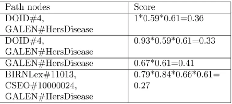
Direct mapping score: 0; number of paths: 4; Aver-age path length:(3 + 3 + 2 + 4)/4 = 3; minimum path length: 2; maximum path length: 4; Average manual mapping: 1/3 because there is only one path of length 3 that contains one manual mapping; For score attributes, we illustrate one (multiplication) of the seven composi-tion funccomposi-tions proposed. We start by computing a score for each path, as shown in Table 1. Then, using these path scores, we compute the following attributes: maxi-mum scores: 0.41; minimaxi-mum scores: 0.27; average scores: (0.36+0.33+0.41+0.27)/4=0.34.
Table 1: Path scores for Figure 6 example.
Path nodes Score
DOID#4, GALEN#HersDisease 1*0.59*0.61=0.36 DOID#4, GALEN#HersDisease 0.93*0.59*0.61=0.33 GALEN#HersDisease 0.67*0.61=0.41 BIRNLex#11013, CSEO#10000024, GALEN#HersDisease 0.79*0.84*0.66*0.61= 0.27 5.2.2. Training data
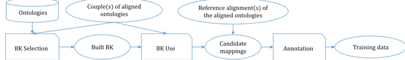
In our case, training data are candidate mappings an-notated by true (correct mapping) or false(incorrect map-ping) and described by all the previously presented at-tributes. As is usual with supervised machine learning, obtaining training data requires previously generated and curated reference alignments from other ontologies than those to align. Preferably, the aligned ontologies are of the same domain as the ontologies to align. To obtain the training data, we propose to apply our approach to the aligned ontologies (i.e., BK selection and BK use). We then, compute the 27 attributes for each derived candi-date mapping and annotate it by true or false according to the reference alignments of the aligned ontologies (see Figure 7).
5.2.3. RandomForest machine learning algorithm
There are several algorithms for learning a classifica-tion funcclassifica-tion from a set of training data. In our exper-iments, we used RandomForest, a non-linear method for classification [6]. In the training step, it learns a multi-tude of decision trees by creating a different random sub-set to train each decision tree. In the classification step, it aggregates the results of these trees by outputting the most frequent class. Due to this strategy, Random Forrest has the advantage of being efficient on any type of data set. Our choice of this algorithm was motivated by its performance in preliminary experiments. Indeed, we eval-uated the classification results produced by different ML
BK Selection BK Use Annotation Couple(s) of aligned ontologies Built BK Candidate mappings Reference alignment(s) of
the aligned ontologies
Training data Ontologies
Figure 7: Training data generation process.
algorithms implemented in the Weka framework [26] such as trees algorithm (J48, RandomForest, RandomTree) and rules algorithms (JRIP, oneR, etc.); RandomForest gener-ated the best results. This confirms the results reported in [28]: for learning linkage rules, the non-linear classifiers (trees) are the most appropriate.
6. Efficiency gain with the built BK
Building a new resource (i.e., the built BK) from the preselected ontologies is more efficient than returning com-plete ontologies as background knowledge. In this section, we estimate the computation time of our BK selection ap-proach and that of the traditional apap-proach, then we com-pare them to demonstrate the efficiency of our approach.
The traditional approach refers to the BK selection methods that match the source and target ontologies to all the preselected ontologies, and then they use the gen-erated alignments to select the ontologies to be exploited as background knowledge [27, 23, 37].
Anchoring is the step that follows BK selection, its computation time depends on the selected BK: a set of ontologies or the built BK. Therefore, we include the an-choring computation time in our comparison. However, we do not include the mapping extraction computation time because it is performed once between the preselected on-tologies independently of the matching tasks. Moreover, when comparing our approach to those that use each BK ontology separately (derivation across only one intermedi-ate concept) [27, 23], the mapping extraction time has a zero value. Indeed, these works do not match BK ontolo-gies between each other.
Let KR = {O1, O2,..., On} be the set of preselected
ontologies, OS the source ontology and OT the target
on-tology, t(M, O1, O2) the function that returns the time
re-quired by the matcher M to align the ontologies O1 and
O2. When using the traditional approach, the selected
BK is a set of k ontologies SR = {SO1,..., SOk}, with
SR ⊆ KR. However, when using our approach, the se-lected BK is one resource built from KR ontologies, called BBK. The BK selection computation-time is computed as follows. • Traditional approach: T1=P n i=1t(M, OS, Oi) +P n i=1t(M, OT, Oi) + α. • Our approach: T10= Pn i=1t(M, OS, Oi) + β.
Where α and β are the computation time required for the treatments performed after the BK selection matching tasks. In the traditional approach, it may be the time of computing similarity measures and ranking the preselected ontologies [27, 23, 37]. In our approach, it is the time of selecting the mappings related to the source ontology and combining them. Usually, the values of α and β are negli-gible comparing to that of the matching tasks performed within the BK selection process.
In the example illustrated in Figure 8, with four prese-lected ontologies, the traditional approach performs eight matching tasks generating the alignments A1 to A8, while
our approach performs four matching tasks generating the alignments A1 to A4.
For the anchoring step, we distinguish two cases: Case 1: Reusing BK selection alignments as anchoring alignments.
The anchoring computation time is computed as follows. • Traditional approach: the anchoring alignments are
already available, no additional matching task is nec-essary.
T2= 0.
• Our approach: The BK selection alignments are re-lated only to the source ontology. Hence, another matching task is necessary to anchor the target on-tology to the BBK (e.g., the time necessary to gen-erate the alignment B2 in Figure 8 (b)).
T20 = t(M, OT, BBK).
The computation time of BK selection and anchoring is estimated as follows. • Traditional approach: T = T1+ T2= n X i=1 t(M, OS, Oi) + n X i=1 t(M, OT, Oi) + α. (1) • Our approach: T0= T10+ T20= n X i=1 t(M, OS, Oi) + β + t(M, OT, BBK). (2)
S T
Traditional approach Our approach
Reusing A1, A3, A5 and A7 alignments
Anchoring to the selected ontologies
S T
Reusing A1, A2, A3 and A4 alignments
T
S T
Anchoring to the Built BK A1 A2 A3 A4 A5 A6 A7 A8 B1 B2 B3 B4 B2 B1 B2 BK selection Selected BK Anchoring ⊕ ⊕
Source ontology Intermediate ontology Target ontology Matching task
S A1 A2 A3 A4 O1 O2 O3 O4 O1 O2 O3 O4 O1 O3 O1 O3 Built BK Built BK Built BK (a) (b)
Case 1 Case 2 Case 1 Case 2
Figure 8: BK Selection and anchoring: Traditional approach vs. our approach
• Comparison: Traditional approach vs. our approach T − T0=
n
X
i=1
t(M, OT, Oi) − t(M, OT, BBK) + (α − β). (3)
Intuitively the difference T − T0 is always positive. In-deed, the difference (α − β) tends to zero, and matching the target ontology to all the preselected ontologies takes more much time than matching the target ontology to the BBK. This intuition is validated with experiments in Sec-tion 8.4.2.
Case 2: The source and target ontologies are anchored to the selected BK with another matcher M0.
In our approach, the anchoring step requires two match-ing tasks, while in the traditional approach, the number of matching tasks depends on the number of the selected BK ontologies. For instance, in Figure 8 (a), with two selected BK ontologies, four matching tasks are necessary to gen-erate B1 to B4. Thus, the anchoring computation time is
computed as follows. • Traditional approach: T2=Pkj=1t(M0, OS, SOj) +Pkj=1t(M0, OT, SOj). • Our approach: T0 2= t(M0, OS, BBK) + t(M0, OT, BBK).
The computation time of BK selection and anchoring is estimated as follows. • Traditional approach: T = T1+ T2= (1) +Pk j=1t(M 0, O S, SOj) +Pkj=1t(M0, OT, SOj). • Our approach: T0= T10+ T20= (2) + t(M0, OS, BBK).
• Comparison: Traditional approach vs. our approach T − T0= (3) +Pk
j=1t(M0, OS, SOj)+
Pk
j=1t(M0, OT, SOj) − t(M0, OS, BBK).
Our hypothesis is that the difference T − T0 is al-ways positive. Indeed, the formula (3) is positive as ex-plained in Case 1, and matching the ontologies to align to the selected BK ontologies (i.e.,Pk
j=1t(M 0, O S, SOj) + Pk j=1t(M 0, O
T, SOj)) takes more time than matching the
source ontology to the BBK (i.e., t(M0, OS, BBK)). Note
that, in our approach, matching the target ontology to the BBK (e.g., generating B2 in Figure 8 (b)) is common to
the two cases, and its computation time is already included in the formula (3). We discussed this case at the end of Section 8.4.2.
7. Experiment materials 7.1. Evaluation datasets
To evaluate our approach, we chose two OAEI tracks: Anatomy and Large biomedical ontology (LargeBio). Our choice was motivated by the fact that, for these tracks,
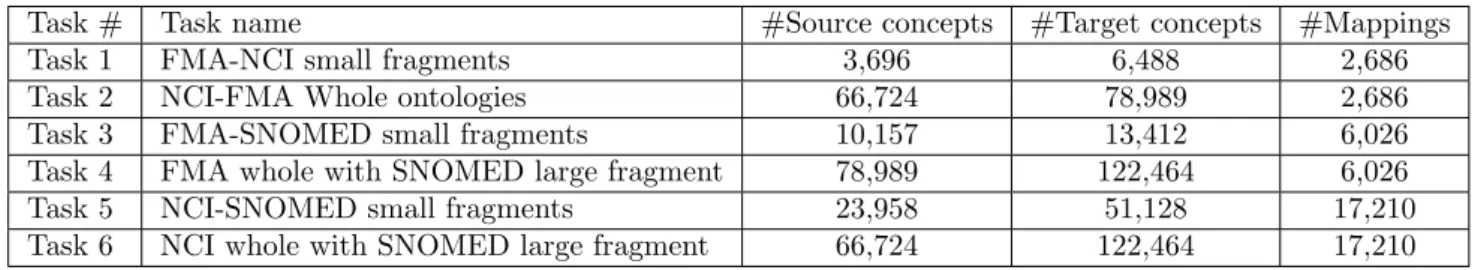
Table 2: LargeBio track (the last column shows the number of mappings in the reference alignment provided by OAEI).
Task # Task name #Source concepts #Target concepts #Mappings
Task 1 FMA-NCI small fragments 3,696 6,488 2,686
Task 2 NCI-FMA Whole ontologies 66,724 78,989 2,686
Task 3 FMA-SNOMED small fragments 10,157 13,412 6,026
Task 4 FMA whole with SNOMED large fragment 78,989 122,464 6,026
Task 5 NCI-SNOMED small fragments 23,958 51,128 17,210
Task 6 NCI whole with SNOMED large fragment 66,724 122,464 17,210
the state-of-the-art systems have used ontologies as back-ground knowledge to enhance the quality of their align-ments. Hence, evaluating using these tracks with the same preselected ontologies allowed us to compare our results to the state-of-the-art’s results.
7.1.1. Anatomy OAEI track
The Anatomy track consists in finding an alignment of 1, 516 mappings between the Adult Mouse Anatomy (2,744 classes) and a subset of the National Cancer In-stitute (NCI) Thesaurus (3, 304 classes) describing human anatomy [14].
7.1.2. LargeBio OAEI track
The Large Biomedical (LargeBio) OAEI track2 aims
at finding alignments between several large and semanti-cally rich biomedical ontologies: the Foundational Model of Anatomy (FMA) [48], National Cancer Institute The-saurus (NCI) [51] and SNOMED Clinical Terms (SNOMED-CT) [12], which contain 78, 989, 66, 724 and 306, 591 con-cepts, respectively. The LargeBio track consists of six tasks corresponding to the different sizes of input ontolo-gies (small fragments/whole ontology of FMA and NCI and small/large fragments of SNOMED-CT; see Table. 2). The Unified Medical Language System (UMLS) [5] has been used as the basis to produce the reference align-ments [7].
7.2. Preselected ontologies
According to the OAEI 2016 campaign, AML [22] and LogMapBio [31] are the best BK-based ontology matching systems. To establish a fair comparison with these sys-tems, our evaluation employs the same set of preselected ontologies as follows:
AML-Ontologies: Three ontologies are preselected for AML: UBERON, DOID and MeSH3. AML makes a
dynamic selection from these ontologies using the Map-ping Gain measure [23].
LogMapBio-Ontologies: In OAEI2016, LogMapBio considered the NCBO BioPortal as the set of preselected
2http://www.cs.ox.ac.uk/isg/projects/SEALS/oaei/ 3MeSH is used as lexicon [21]
ontologies. LogMapBio selected 10 ontologies for each matching task. For our evaluation, we considered the com-bination of all the ontologies selected by LogMapBio as the preselected ontologies in order to establish a fair final re-sult comparison. The combination yields 21 ontologies. However, YAM++ could not parse three of those ontolo-gies. Indeed, these ontologies require importing external ontologies, a process which is not managed by YAM++. Thus, we ended up using 18 (out of the 21) ontologies for our comparison with LogMapBio. These ontologies are listed in Table 3 with their NCBO BioPortal acronyms4.
For each matching task, we name BBK1 the back-ground knowledge resource built from AML-Ontologies and BBK2 the one built from LogMapBio-Ontologies. Build-ing the BK is performed accordBuild-ing to the process described in Section 3 with YAM++ as a matcher. The extracted mappings, the candidate mappings, as well as the source code are openly available5.
7.3. Tools and resources
YAM++. We used YAM++ to generate all the re-quired alignments for our experiments. YAM++ is an on-tology matching system previously developed by our team at LIRMM6 [41]; it does not rely on a specialized BK to match biomedical ontologies. It is considered as one of the state-of-the-art ontology matching systems, and was the top ranked system in OAEI 2013. YAM++ combines sev-eral syntactic, lexical and structural similarity measures.
OBO x-refs. In addition to the mappings generated by YAM++, we also extracted cross-reference properties from the preselected ontologies when available (i.e., from the preselected ontologies present in the OBO Foundry). As previously pointed out (see Section 3.2), these cross-references may be considered as manually curated pings. Therefore, we added them to the extracted map-pings and assigned them a score of 1 when computing can-didate mapping scores.
4These ontologies are accessible on NCBO BioPortal with the link
https://bioportal.bioontology.org/ontologies/ontologyAcronym
5https://github.com/AminaANNANE/BK-based-matching 6http://www.lirmm.fr/yam-plus-plus
Table 3: LogMapBio-Ontologies (ontologies tagged by * could not be parsed by YAM++).
N◦ Ontology acronym Number of concepts
1 BIRNLEX 3,580 2 BTO 5,902 3 CCONT 19,991 4 CL* 2,352 5 CLO 40,884 6 CSEO 20,085 7 DDO* 6,444 8 DINTO* 28,178 9 DOID 12,432 10 EFO 19,909 11 EHDAA2 2,772 12 GALEN 23,141 13 HP 15,804 14 MA 3,257 15 ONTOAD 5,899 16 RCTV2 88,854 17 SYN 14,462 18 UBERON 19,761 19 VHOG 1,185 20 XAO 1,621 21 ZFA 3,168
Neo4j. Technically, the mapping filtering step pro-duces two files: (i) an OWL file containing all selected con-cepts with their labels and ontology source, and (ii) a CSV file containing all mappings in format (URI source, URI ontology source, URI target, URI ontology target, score, manualMapping). manualMapping is a boolean property that takes ”true” or ”false” as value. The OWL file is used for anchoring the target ontology to the built BK. The mapping file is stored as a graph database using Neo4j7,
where each node is unique and described by its URI and ontology source. A graph database facilitates the deriva-tion step. Indeed, with reladeriva-tional databases, one has to implement an algorithm and perform several queries to find all paths between a given source and target concepts. Instead, with a graph database, which is intrinsically de-signed to work with paths within graphs, a single simple query is sufficient.
Weka. Weka8is an open source software that includes a collection of machine-learning algorithms for data min-ing tasks. We used the RandomForest algorithm included in Weka [26].
Machine specifications. We run our experiments on an HP ZBook computer that has an Intel Core i7-4910MQ processor, 2.90 GHz of clock, 32 GB of RAM, and a 64-bit Operating System (Windows 8.1 pro).
7https://neo4j.com/
8https://www.cs.waikato.ac.nz/ml/weka/
8. Experimental evaluation
In this section, we evaluate our BK-based ontology matching approach through several experiments. We orga-nize the evaluation in five sections. Each section is intro-duced with an assumption that we try to validate through experiments.
8.1. Assumption 1: Our BK selection method builds a smaller-size BK than the preselected ontologies As discussed previously, our BK selection approach does not return a set of ontologies. Instead, it builds a BK that combines concepts selected from the various pre-selected ontologies. To verify the assumption of this sec-tion, we compare the size (i.e., the number of concepts) of our built BK with that of the preselected ontologies (i.e., AML-Ontologies and LogMapBio-Ontologies).
In Table 4, for each matching task, we present the size of the built BK (BBK1 or BBK2) in number of concepts. Furthermore, we compute a percentage by dividing the size of the built BK by the size of the preselected ontologies. BBK1 is built from three ontologies, which have a global size of 297, 031 concepts while BBK2 is built from 18 on-tologies, which have a global size of 302, 707 concepts. For instance, the size of Task 1 BBK1 is 6, 809; dividing 6, 809 by 297, 031 gives a percentage of 2%, which means that the BBK1 size represents only 2% of the preselected ontologies size.
The results reported in Table 4 validate Assumption 1. Indeed, for all matching tasks, the size of the built BK is much smaller than the size of the preselected ontologies. The percentage varies from one task to another with re-spect to the size of the ontologies to align. Tasks 2 and 6 share exactly the same built BK because they have the same source ontology (see Table 2); this shows that, when matching the source ontology with several target ontolo-gies, the BK selection step may be performed once, and the built BK can be reused for each target ontology.
Table 4: Size comparisons: built BK vs. preselected ontologies.
Task BBK1 size BBK2 size
Anatomy 3,173 1% 11,090 4% Task 1 6,809 2% 18,104 5% Task 2 46,280 15% 48,521 16% Task 3 13,036 4% 27,465 8% Task 4 16,251 5% 34,626 10% Task 5 12,895 4% 36,456 12% Task 6 46,280 15% 48,521 16%
8.2. Assumption 2: Deriving mappings across several intermediate concepts generates more correct map-pings than deriving across one intermediate concept. Deriving candidate mappings is performed by search-ing paths between source and target concepts. Each path contains a number of intermediate concepts belonging to
the preselected ontologies. For instance, with three pre-selected ontologies, we may derive mappings with paths that contain one intermediate concept, two intermediate concepts and three intermediate concepts. In these exper-iments, we derived mappings with a maximum of three in-termediate concepts. Indeed, according to our experiments in [3], deriving mappings with more than three interme-diate concepts generates much more incorrect mappings than correct ones.
To verify that deriving mappings across several inter-mediate concepts generates more correct mappings, we derived all possible candidate mappings between the on-tologies to align for each matching task. We then com-puted (1) A: the number of correct mappings derived with only paths containing one intermediate concept; (2) B: the number of correct mappings derived with paths containing one, two and three intermediate concepts: (3) Gain: the percentage of gain when using paths with several interme-diate concepts (Gain = B−AA ). The results are reported in Table 5.
As we can see, Assumption 2 is validated. Indeed, for each matching task, the derivation across several interme-diate concepts generates more correct mappings, with a gain of up to 7%, compared to deriving mappings with only one intermediate concept. Tasks 1 and 2 have the same values, since they have the same reference align-ment. The same is true for Tasks 3 and 4, Tasks 5 and 6. Note that deriving mappings with only one intermediate concept is comparable to deriving with each BK ontology independently (i.e, separately from the other BK ontolo-gies, composing only two anchoring mappings related to the same BK ontology), which is the method adopted by almost all related works [22, 30, 27, 46]. Instead, thanks to the mapping extraction task, our approach combines all preselected ontologies.
For Anatomy, the gain is not significant. This may be explained by the use of UBERON, which is an integrative multi-species anatomy ontology. Indeed, UBERON, em-ployed as the only BK ontology, allows to identify more than 80% of Anatomy reference alignment mappings.
When deriving mappings across several intermediate concepts, we may notice that the number of correct map-pings derived with BBK1 is comparable to BBK2 for Tasks 1, 2, 3 and 4. However, for Tasks 5 and 6, the gap is larger: 10, 315 correct mappings are derived with BBK2 while only 5, 091 correct mappings are derived with BBK1. This shows that BBK2 is more effective than BBK1 for these tasks.
8.3. Assumption 3: Our rule-based and ML-based mapping-selection methods are effective
Exploiting background knowledge resources in ontol-ogy matching generates more correct and incorrect map-pings (as previously discussed), selecting the most relevant mappings is a crucial step. We proposed and described two mapping selection methods in Section 3. Here we evaluate these methods to validate Assumption 3.
Table 5: Evaluation of derivation effectiveness using several interme-diate concepts.
BK Task A B Gain
BBK1
Anatomy 1,403 1,405 0.1%
Task 1 & Task 2 1,938 2,054 6.0% Task 3 & Task 4 2,043 2,158 5.6% Task 5 & Task 6 4,789 5,091 6.3%
BBK2
Anatomy 1,411 1,420 0.6%
Task 1 & Task 2 2,369 2,442 3.1% Task 3 & Task 4 2,511 2,685 6.9% Task 5 & Task 6 9,871 10,315 4.5%
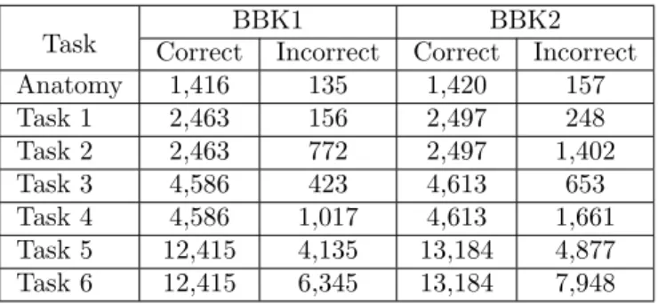
Table 6: Correct and incorrect mappings in the baseline.
Task CorrectBBK1Incorrect CorrectBBK2Incorrect
Anatomy 1,416 135 1,420 157 Task 1 2,463 156 2,497 248 Task 2 2,463 772 2,497 1,402 Task 3 4,586 423 4,613 653 Task 4 4,586 1,017 4,613 1,661 Task 5 12,415 4,135 13,184 4,877 Task 6 12,415 6,345 13,184 7,948
To carry out our experiments, we employed the follow-ing mappfollow-ing selection methods:
1. Baseline. This is the simplest method. It keeps all candidate mappings that have been derived without any selection. In Table 6, we present the number of correct and incorrect mappings in the baseline. 2. Rule-based selection. This method implements
the rules described in Section 5.1 to select the final mappings.
3. ML-based selection. To evaluate ML mapping se-lection, we implemented two strategies which use the same ML algorithm (RandomForest) and the same attributes to describe candidate mappings but for which we generate training data differently. Note that, in both strategies, test data (candidate map-pings to classify) and training data are completely distinct.
(a) Cross validation. This strategy is often used to evaluate the performance of the ML algo-rithm and the attributes when using training data objects that are similar to the objects to classify. The process for a given matching task is as follows: (1) we randomly subdivide the set of candidate mappings of this task into two equal subsets. (2) Based on the reference align-ment, we annotate the candidate mappings of the first subset with true or f alse. (3) We use the annotated subset as training data to learn a classifier. (4) We then classify the can-didate mappings of the second subset with the resulting classifier. (5) We interchange the two
0.600 0.650 0.700 0.750 0.800 0.850 0.900 0.950 1.000 AN A T O M Y TA S K1 TA S K2 TA S K3 TA S K4 TA S K5 TA S K6 F-MEASURE
Baseline Rule based Cross validation Separate learning
c
0.600 0.650 0.700 0.750 0.800 0.850 0.900 0.950 1.000 AN A T O M Y TA S K1 TA S K2 TA S K3 TA S K4 TA S K5 TA S K6 PRECISIONBaseline Rule based Cross validation Separate learning
a
0.6 0.65 0.7 0.75 0.8 0.85 0.9 0.95 1 AN A T O M Y TA S K1 TA S K2 TA S K3 TA S K4 TA S K5 TA S K6 RECALLBaseline Rule based Cross validation Separate learning
b
Figure 9: Evaluation of mapping selection methods using BBK1.
subsets such that we annotate the second sub-set and classify the candidate of the first one. (6) Finally, we combine the two classification results (taking all the candidate mappings clas-sified as true) to obtain the final alignment. (b) Separate learning. Here, we generate the
training data for a given matching task using the ontologies and reference alignments of other tasks. For LargeBio, we adopt a leave-one-out strategy. For each task, we generate the traing data ustraing other same-size tasks. For in-stance: there are three large fragments tasks (Tasks 2, 4 and 6), to classify Task 2 candi-date mappings, we use the ontologies and ref-erence alignments of Tasks 4 and 6 to generate the training data, according to the process illus-trated in Figure 7. For Anatomy, we generated
0.600 0.650 0.700 0.750 0.800 0.850 0.900 0.950 1.000 AN A T O M Y TA S K1 TA S K2 TA S K3 TA S K4 TA S K5 TA S K6 F-MEASURE
Baseline Rule based Cross validation Separate learning
f
0.6 0.65 0.7 0.75 0.8 0.85 0.9 0.95 1 AN A T O M Y TA S K1 TA S K2 TA S K3 TA S K4 TA S K5 TA S K6 PRECISIONBaseline Rule based Cross validation Separate learning
d
0.6 0.65 0.7 0.75 0.8 0.85 0.9 0.95 1 AN A T O M Y TA S K1 TA S K2 TA S K3 TA S K4 TA S K5 TA S K6 RECALLBaseline Rule based Cross validation Separate learning
e
Figure 10: Evaluation of mapping selection methods using BBK2.
the training data with Tasks 1, 3 and 5. In this section, to evaluate the performance of our selec-tion methods fairly, we compute the recall with respect to the number of derivable correct mappings but not to the number of mappings in the reference alignment. Indeed, if some correct mappings are not available in the set of can-didate mappings, we cannot blame the selection method for not having returned them.
Recall = T P GT P
Where T P is the number of the correct mappings re-turned by a given selection method, and T P G is the num-ber of all correct mappings derivable with the built BK.
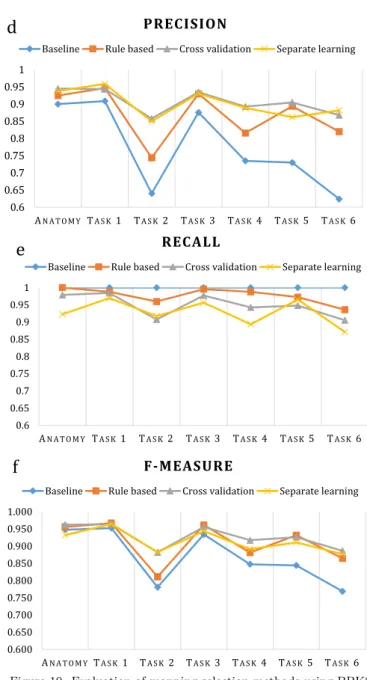
Figures 9 and 10 present the results of our experiments for each matching task exploiting respectively BBK1 and BBK2. In particular, we show the precision, recall and
F-measure of the produced alignments to observe the be-havior of each mapping selection method.
Precision: As we can see in Figures 9 (a) and 10 (d), the baseline’s precision for small size tasks (Task 1, Task 3 and Anatomy) is comparable to that of other selection methods. However, for larger size tasks (Tasks 2, 4, 5 and 6), the precision is low, especially for Tasks 2 and 6. Even if the precision curves display the same trend in Figures 9 (a) and 10 (d), the scores in Figure 10 (d) are lower than those in Figure 9 (a). This may be explained by the fact that BBK2 is built from a larger number of preselected ontologies than BBK1 18 vs. 3 ontologies). Hence, BBK2 generates more correct (see Table 5) and incorrect mappings, which decreases precision. The ML-based selection methods consistently yields higher preci-sion than the rule-based selection method, with an average of 0.915 for cross-validation and 0.909 for separate learn-ing (vs. 0.881 for the rule-based selection). The largest gap is observed in Task 2. This is due to the fact that the NCI Thesaurus includes a small branch on mouse anatomy (in addition to the human anatomy branch). Using the cross-references extracted from UBERON (considered as manual mappings) and the selection rule number 2 (see Section 3), the rule-based selection method returns map-pings between human and mouse anatomy. However, the UMLS, the source from which the reference alignment is extracted, is focused only on human health, and does not include mappings between the NCI mouse anatomy branch and MA; therefore, these mappings are considered as in-correct, which affects precision.
Recall: The baseline always shows a recall of 1, be-cause we computed a customized recall as described above (see Figures 9 (b) and 10 (e)). Our selection methods yield a high recall in all matching tasks. The rule-based mapping selection method obtained the best recall scores, with an average of 0.979, while the cross-validation and separate-learning methods have a recall average of 0.955 and 0.938, respectively. The difference between the rule-based and separate-learning selection is significant in Task 4, while the gap is smaller with cross-validation. This may be explained by the low precision of the baseline alignment of Tasks 2 and 6. This affects the learned classifier. Indeed, the baseline alignments of Tasks 2 and 6 are the train-ing data of Task 4. Traintrain-ing data contains many f alse candidate mappings increase the probability of classifying a given candidate mapping as f alse, which, in turn, de-creases recall.
F-measure: We present the F-measure values in Fig-ures 9 (c) and 10 (f). The cross-validation method yielded the best F-measure scores with an average of 0.942 when using BBK1 and of 0.928 when using BBK2. These results demonstrate that the ML technique with the proposed at-tributes and similar data training is effective for mapping selection. ML-based mapping selection is therefore par-ticularly well-suited for complementing an existing partial alignment between two ontologies (the partial alignment may be used to generate the training data) [34, 38], or for
matching new ontology versions when an alignment be-tween the old ontology versions already exist. Indeed, the training data may be generated with the existing align-ment.
The separate-learning method produced high F-measure scores as well, close to the cross-validation method’s scores, with an F-measure average of 0.931 and 0.914 when using BBK1 and BBK2, respectively. These results are more in-teresting. They represent a concrete case where we may reuse existing alignments within the same domain to learn an effective classifier. Note that, we generated the training data for the Anatomy (that has a gold standard reference alignment) using alignments extracted automatically from UMLS (Tasks 1, 3 and 5 reference alignments), and the selection results are promising.
The rule-based method provides results with an av-erage of 0.931 and 0.910 when using BBK1 and BBK2, respectively. It obtained the best F-measure values for the small tasks (i.e., Anatomy, Tasks 1 and 3). However, its performance decreases (i.e., achieves lower precision) for large tasks, compared to ML-based selection, which is more stable.
The results of the ML-based and rule-based mapping selection methods are comparable in terms of F-measure scores. However, the ML-based selection promotes preci-sion, while the rule-based selection promotes recall.
Rule-based mapping selection is simple and efficient but static. Indeed, although each ontology-matching task has its own specificities (for instance, the best threshold value varies from one task to another), the same rules ap-ply all the time. ML-based mapping selection is time con-suming and requires aligned ontologies to generate training data. However, it dynamically learns a customized classi-fier that combines multiple selection attributes (27 in our case). Mappings that are manually created or validated stored in platforms such as YAM++ online [4]9, NCBO
BioPortal or resources such as OBO ontologies may be used to generate training data.
Based on our experiment results, we can validate As-sumption 3. Our selection methods are effective: they sig-nificantly improve baseline precision and consistently keep high recall.
8.4. Assumption 4: The use of ontologies as background knowledge has a computation time cost and our built BK reduces this cost
In this section, we describe our computation time eval-uation. We start by analyzing and discussing the time necessary to perform each step of our approach. We then present the efficiency gain obtained.
8.4.1. Computation time evaluation of our approach: step by step
Figures 11 and 12 present the time, in minutes, re-quired for the different steps in our approach.
0 20 40 60 80 100 120 140 ME Anatomy Task 1 Task 2 Task 3 Task 4 Task 5 Task 6
ME:Mapping Extraction Mapping filtering Mapping combination
Anchoring Derivation Direct matching
Figure 11: BK selection and BK use computation time in minutes (BBK1). 0 20 40 60 80 100 120 140 ME Anatomy Task 1 Task 2 Task 3 Task 4 Task 5 Task 6
ME:Mapping Extraction Mapping filtering Mapping combination
Anchoring Derivation Direct matching
Figure 12: BK selection and BK use computation time in minutes (BBK2).
BK selection
The BK selection step includes three tasks: mapping extraction, mapping filtering and mapping combination.
Mapping extraction is the costliest task in terms of computation time, especially when using a large number of preselected ontologies, as is the case for BBK2 (18 on-tologies). Indeed, extracting the mappings from the AML-Ontologies and LogMapBio-AML-Ontologies took 77 and 132 minutes, respectively. Fortunately, this task is performed independently of matching tasks. In fact, for a given set (or repository) of preselected ontologies, the mapping ex-traction task is performed only once whereas its output (the set of alignments) is reused for any matching task. Therefore, we report the computation time of the mapping extraction process once for all matching tasks in Figures 11 and 12.
BBK1 is built from three ontologies. However, the time necessary for extracting the mappings from the three on-tologies is 58% the time necessary for performing the same process from 18 ontologies. This may be explained by the fact that, in terms of computation time, matching a large preselected ontology such as MeSH is equivalent to
match-ing several small ontologies.
The high computation time cost of the mapping extrac-tion step is justified by the fact that the mapping deriva-tion across several intermediate concepts generates more correct mappings, as demonstrated in Section 8.2.
Mapping filtering is the second costliest process. It includes two tasks: (i) matching the source ontology to the preselected ontologies and (ii) selecting the mappings related to the source ontology. The first task is time-consuming, especially when dealing with large scale on-tologies such as MeSH. Indeed, it is surprising to notice that matching the source ontology to 3 preselected ontolo-gies takes more time than matching it to 18 preselected on-tologies (see Figures 11 and 12). MeSH contains 265, 414 concepts, and each concept is described with multiple la-bels. Therefore, YAM++ takes long time to match MeSH with the source ontology, particularly when the latter is a large-scale one. The second task takes only few seconds in all cases.
Mapping combination is performed with Neo4j allow-ing us to merge the same nodes of different mappallow-ings. It takes less than 2 seconds in all cases.
BK use
This step consists in exploiting the built BK to derive candidate mappings (anchoring and derivation). It takes much less time than the BK selection step. The size of the target ontology is larger than that of the source ontology (see Table 2), however, we notice that anchoring the target ontology takes less time than matching the source ontology to the preselected ontologies in the mapping filtering step. This may be explained by the fact that the target ontology is anchored only to the reduced-size built BK.
The derivation task is performed with Neo4j. It takes less than one minute for small matching tasks and up to three minutes for large ones.
Final mapping selection
The computation time for the rule-based mapping se-lection method is less than two seconds in all cases. How-ever, when using ML-based selection, computation time is much longer. This is mainly due to the generation of training data. For example, in our evaluation, we used Tasks 1 and 3 to generate the training data for classifying Task 5 candidate mappings. Hence, the time necessary to generate the training data in this case is the time neces-sary for BK selection and BK use of Tasks 1 and 3. Note that the training data for Task 5 may be generated with Task 1 only. Furthermore, the learned classifier is reusable in the same domain. Indeed, we tried to classify Task 4 candidate mappings derived from BBK2 with the classi-fier trained with Tasks 2 and 6 candidate mappings derived from BBK1. We obtained almost the same results as those obtained with the classifier trained with candidate map-pings derived from BBK2. Hence, spending time to learn one classifier for a given domain is acceptable, because it can be reused for different matching tasks. Learning a classifier and classifying candidate mappings are less time consuming and take only few seconds.
Comparing the time necessary for direct matching to that required for BK-based matching shows that the use of BK in ontology matching is time-consuming.
8.4.2. Efficiency gain with the built BK
Our approach reduces the computation time of the BK-based matching process, especially that of BK selection and anchoring as explained in Section 6. In our evaluation we used the same matcher (i.e., YAM++) for BK selec-tion and anchoring. Hence, we are in Case 1 that reuses the BK selection alignments as anchoring alignments. We compare T and T’ computed according to the formulas (1) and (2) introduced in Section 6, respectively.
In Figures 13 and 14, we present: (i) T: the time neces-sary for matching the source and target ontologies to the preselected ontologies in the traditional approach. We ig-nore α because it has a small value and variates from one work to another as explained in Section 6; (ii) T’: the time necessary for mapping filtering, mapping combination and anchoring the target ontology to the built BK in our ap-proach, and (iii) the percentage ratio comparing the two. This ratio is computed by dividing T0 by T .
In all cases, our approach is more efficient than the traditional approach (i.e., T0 < T ). The gain is between 42% (for Task 2 with BBK1) and 60% (for Task 4 with BBK2). These results are expected since T and T’ have a common part: matching the source ontology to the prese-lected ontologies. However, matching the target ontology to the preselected ontologies takes more time comparing to matching the target ontology to the BBK. For instance, in all tasks, matching the target ontology to BBK1 takes less than four minutes, while matching the target ontology to the large ontology MeSH always takes about 30 minutes.
With YAM++, the average time to match an ontology of LargeBio or Anatomy to: (i) one of the 18 ontologies listed in Table 3 is 2.8(min), (ii) the BK built from the 18 ontologies is 5.5(min). We may use these values to check our intuition about the efficiency gain in Case 2. When selecting only one ontology as background knowledge from the 18 ontologies, the difference between T and T’ in Case 2 is computed as follows.
T − T0 = E + (2.8 + 2.8) − 5.5 = E + 0.1(min) where E is the value of the formula (3) that is the difference between T and T0 in Case 1. As we can see in Figure 13 and 14, E is always positive. Hence, E + 0.1(min) is positive.
In Case 2, the efficiency gain becomes more significant as the number of selected ontologies increases. For in-stance, with two ontologies as BK, the difference becomes: T − T0 = E + (2.8 ∗ 2 + 2.8 ∗ 2) − 5.5 = E + 5.7(min)
Based on the obtained results, we conclude that our BK selection approach builds an efficient BK, which val-idates Assumption 4. Indeed, the built BK reduces the BK selection and anchoring computation-time comparing to the traditional approach.
0% 10% 20% 30% 40% 50% 60% 70% 0 20 40 60 80 100 120 140
Anatomy Task 1 Task 2 Task 3 Task 4 Task 5 Task 6 T (traditional appraoch) T' (our approach) Ratio
Figure 13: Efficiency gain with BBK1.
0% 10% 20% 30% 40% 50% 60% 70% 0 20 40 60 80 100 120 140
Anatomy Task 1 Task 2 Task 3 Task 4 Task 5 Task 6 T (traditional appraoch) T' (our approach) Ratio
Figure 14: Efficiency gain with BBK2.
8.5. Assumption 5: The small size of the built BK does not affect its effectiveness
According to OAEI campaigns [17], AML and LogMap-Bio are the best systems using ontologies as background knowledge. To verify the effectiveness of the built BK, we compare our results to theirs. For a fair comparison, (i) our evaluation uses the ontologies that were preselected for these systems in the OAEI 2016 campaign, (ii) only our rule-based selection results are compared since the OAEI rules prohibit training on OAEI datasets10, and (iii) we re-paired the alignments generated by our approach with the LogMap’s ontology repair module (LogMap-Repair) [32], which is available as a self-contained software component11. Indeed, AML and LogMapBio use logical repair strategies to ensure the coherence of their alignments.
The aim of this comparison is to evaluate the perfor-mance of our approach regarding the best results obtained using the same preselected ontologies. Thus, if we obtain comparable results, we can conclude that the reduced size of the built BK does not affect its effectiveness.
Note that, in this section, we compute the recall against the reference alignment, as described in Section 2.2.
In Table 7, we present the difference between the F-measure values of the repaired alignments and those of
10http://oaei.ontologymatching.org/doc/oaei-rules.2.html 11https://code.google.com/archive/p/logmap-matcher/downloads