HAL Id: hal-02270420
https://hal.archives-ouvertes.fr/hal-02270420
Submitted on 25 Aug 2019HAL is a multi-disciplinary open access archive for the deposit and dissemination of sci-entific research documents, whether they are pub-lished or not. The documents may come from teaching and research institutions in France or abroad, or from public or private research centers.
L’archive ouverte pluridisciplinaire HAL, est destinée au dépôt et à la diffusion de documents scientifiques de niveau recherche, publiés ou non, émanant des établissements d’enseignement et de recherche français ou étrangers, des laboratoires publics ou privés.
Incremental Validation of Real-Time Systems
D. Doose, Zoubir Mammeri
To cite this version:
D. Doose, Zoubir Mammeri. Incremental Validation of Real-Time Systems. 3rd European Congress on Embedded Real Time Software - ERTS 2006, Jan 2006, Toulouse, France. �hal-02270420�
Incremental Validation of Real-Time Systems
D. Doose, Z. Mammeri
IRIT Paul Sabatier University, Toulouse France
Abstract: Real-time embedded systems are used in highly important or even vital tasks (avionic and medical systems, etc.), thus having strict temporal constraints that need to be validated. Existing solutions use temporal logic, automata or scheduling techniques. However, scheduling techniques are often pessimistic and require an almost complete knowledge of the system, and formal methods can be ill-fitted to manipulate some of the concepts involved in real-time systems.
In this article, we propose a method that has the advantages of formal methods and some simplicity in manipulating real-time systems notions. This method is able to model and validate all the classical features of real-time systems, without any pessimism, while guaranteeing the end of the validation process. Moreover, its formalism enables to validate systems of which we have only a partial knowledge, and thus to validate or invalidate a system still under design. This latest point is very important, since it greatly decreases the cost of design backtracks.
Keywords: real-time systems, validation, partial knowledge, polyhedra.
1. Introduction
Validation is a mandatory step in critical real-time systems design, and can be important even for non-critical ones. There are many ways to check the temporal behavior of a real-time system: we can use formal methods based on logic (LTL, CTL, etc.) or automata [1, 2, 3] (Petri nets, linear hybrid automata, etc.), or we can use scheduling techniques [7] (RMA method, etc.). Methods based on logic give precise results and have a great expressive power. They can model very specific features, but involve a strenuous designing process. Indeed, they are not initially fitted to the particular case of real-time system validation, and notions such as tasks or resources sharing do not exist in Petri nets or linear hybrid automata. Scheduling techniques have two main advantages. Firstly, they are of course completely fitted to real-time systems. Secondly, they usually have a very low complexity. However, they often are pessimistic, they require an almost complete knowledge of system parameters (tasks periods, priorities, precedence relationships, etc.), and they give quite
limited results, confined mostly to the possible schedulability of the system.
Our goal is to combine formal methods and scheduling techniques by devising a method fitted for scheduling analysis while preserving the expressivity and precision of formal methods such as linear hybrid automata [10, 11, 12].
The analysis of linear hybrid automata solvers led us to the use of polyhedral domains, that enable a powerful modeling and checking. This way, we devised the only method (as far as we know) that brings together the following features:
• It can model and analyse classical features of real-time systems (tasks, resources sharing, precedence, atomic task executions, etc).
• It guarantees the ending of the validation process (decidability), contrary to linear hybrid automata [9, 13].
• It is non-pessimistic.
• It gives precise results on the behavior of the system: we can deduce the response times of tasks, preemptions between tasks, etc., and of course the schedulability of the system.
• It enables to validate/invalidate systems under partial knowledge. Moreover, any parameter constraint (value or linear equation on parameter value) is taken into account by the model. The ability to check a system schedulability during its design (``under partial knowledge'') can lead to important savings by avoiding backtracks. Besides, the non-pessimism implies that we can avoid system over-sizing. Lastly, since the method core works by computing all the different possible behaviors of a system, we can highlight the fact that it is similar to the use of an exhaustive set of simulations, while being far less time-consuming.
The paper is structured as follows: in section two, we introduce the notion of polyhedra and the PV-domains. In section three, we describe our method. In section four, we propose an example comparing the proposed method and a simple schedulability analysis. Finally, we conclude in section five.
2. Notion of Polyhedra 2.1. Polyhedron
The model we propose allows to taking into account any constraint based on linear inequalities. It uses polyhedra [14, 15, 19] to represent the parameters and the properties of the real-time system under construction.
Definition 1: A polyhedron P is the intersection of a
finite family of closed linear half-spaces of the form
{
x
ax
≥
c
}
where a is a non-zero row vector and c is a scalar constant.2.1.1. Double representation
A polyhedron has a dual representation: an implicit representation and a parametric representation. Indeed, a polyhedron P can be represented with a set of linear inequalities which represent its constraints. Its implicit definition is the following one:
{
x
Ax
b
Cx
d
}
P
=
=
,
≥
[1], where A and C are matrices and x, b and d are vectors.
The parametric representation of the polyhedron is the following one:
{
+
+
≥
∑
=
}
=
x
L
λ
R
µ
V
ν
,
µ
,
ν
0
,
ν
0
P
[2], where the polyhedron is composed of several lines (columns of the matrix L), a convex combination of vertices (columns of the matrix V), and a combination of external rays (columns of the matrix R).
Algorithms exist to compute the second representation from the first one, and reciprocally. Both representations are useful. Indeed, the implicit representation is more intuitive, so we use it to represent the different constraints of the system and the results of the validation. However, the parametric representation is more efficient to compute the operations on polyhedral domains. Thus, we will use algorithms based on the dual representation, which computes both representations simultaneously. 2.1.2. Polyhedral domain
We mainly use two operations on polyhedra: intersection and union of polyhedra. Contrary to the intersection, the result of a polyhedra union may not be a convex polyhedron. That is why the notion of polyhedral domain is needed.
Definition 2: A polyhedral domain D of dimension n is
defined as
D
{
i
i
ni
P
}
nP
I
Ζ
=
⊂
Ζ
⊂
,
:
where Pis a union of polyhedra of dimension n.
2.2. PV-domain
We introduce a new notion that aims to create a link between the variables corresponding to the system parameters and their polyhedral representation. A PV-domain (Polyhedral representation of Variables) is composed of a vector of variables (V) and a polyhedral domain (S). The variables can either be a value or a dimension of the polyhedral domain. 2.2.1. PV-domain operations
Adding a variable consists in adding a space dimension at the end of the polyhedral domain and adding a variable to the variables list V, noted:
{ }
v
D
D
'
=
+
[3]Removing a variable consists in removing the variable from the list and removing the corresponding dimension in the polyhedral domain:
{ }
v
D
D
'
=
−
[4]Reducing the PV-domain consists in modifying each variable of the list representing a dimension which has a unique value in the polyhedral domain (
∀
v∈V∀
p∈S,
{
v
=
a
}
⊂
p
) by removing the corresponding dimension in the polyhedral domain and transforming the variable representing a dimension into a variable representing the value:)
(
'
D
D o
=
[5]The intersection (resp. union) of the PV-domain
(
V
S
)
D
=
,
andD
'
=
(
V
,'
S
'
)
is noted∩
(resp.∪
) and defined as follows:(
,
'
)
'
V
S
S
D
D
∩
=
∩
[6]Applying constraints from a variable x to a variable y of a PV-domain D consists in adding the constraints linked to first the variable to the second variable1. This operation is done through a preimage between
x and y and it is noted
apply
(
D
,
x
,
y
)
.The intersections and disjunctions are allowed between two PV-domains if and only if they are compatible. Two PV-domains are compatible if:
(
V
i
is
a
value
V
i
is
a
value
)
i,
[
]
⇔
'
[
]
∀
[7]2.2.2. Efficiency
The complexity and thus the computation time of intersections (resp. unions) of polyhedra depends (exponentially) on their space dimension. That is why the main objective is to reduce as much as possible the space dimension of the system model.
1 The variable y cannot be a value, it must
correspond to a space dimension of the PV-domain. If x is a value, then y becomes the same value.
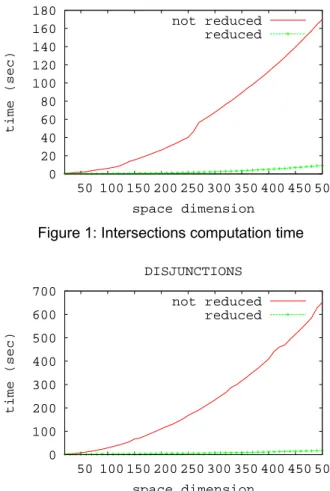
The real efficiency of the space reduction made by the PV-domain reduction operator can be shown by simulations. The simulations on Figure 1 and 2 are run on one polyhedron with ten unknown dimensions and from 20 to 500 space dimensions. In each case (i.e. for each total number of dimensions), we run 500 intersections (resp. unions) with and without using the space dimension reduction. The computation time of the unions is due to the polyhedra power-set operations used for the representation of the disjunctions. We can see here how efficient the dimension reduction can be, but it is important to notice that the dimension reduction is not an invertible operation.
0 20 40 60 80 100 120 140 160 180 50 100 150 200 250 300 350 400 450 500 time (sec) space dimension INTERSECTIONS not reduced reduced
Figure 1: Intersections computation time
0 100 200 300 400 500 600 700 50 100 150 200 250 300 350 400 450 500 time (sec) space dimension DISJUNCTIONS not reduced reduced
Figure 2: Disjunctions computation time 3. The proposed method
The analysis of real-time systems with the proposed method has three main parts.
The first part consists in taking into account the knowledge of the system by: adding the tasks of the system, modifying the static parameters, adding the tasks constraints and finally verifying preconditions. The second part consists in determining all the possible groups of task instances. The notion of group will be detailed later.
The last part consists in validating the previously created groups. The result of the validation process gives to the designer a complete knowledge of the possible behaviors of the systems. Thus, we can deduce the schedulability of the system.
At the end of this section we present the main algorithm of the method and we explain why it is not pessimistic and why it guarantees the end of the validation process.
3.1. System Information
In this first part of the method we design the system through:
• A PV-domain representing the constraints on the parameters of the system (noted system). • A set of static parameters about the system. 3.1.1. Adding Tasks
The first step consists in adding the tasks of the system to its representation. Thus, by knowing the number of tasks we can determine the space dimension of the PV-domain which contains the tasks parameters. The parameters of the task i are: • its release time, noted Ri;
• its priority, noted P i;
• its execution time, noted Ci;
• its period (if the task is periodic), noted Ti;
• its relative deadline, noted Di.
It is important to notice that Ci doesn’t represent the
worst case execution time of the task but merely its execution time. That is why, we can take into account system information more precisely.
At the end of this step, the system is the following universe PV-domain:
=
universe
D
T
C
P
R
D
T
C
P
R
system
n,
n,
n,
n,
n,
,...,
,
,
,
,
0 0 0 0 0 [8]3.1.2. Adding static information
This step consists in modifying the static parameters. A parameter is static (in the particular context of the method proposed in this article) if it represents a piece of information about the design of the system. For example, if a resource is needed for the execution of a task, then the static parameters of the system contain this resource, the fact that this task needs the resource and the access protocol of the resource [4, 18] (Mutex, PIP, PCP, SRP, etc.). During this step the designer also determine the scheduler of the system which is a static parameter too. The proposed method can handle different scheduler based on fixer or dynamic priorities. We will detail this point later.
3.1.3. Adding parameter information
In a third step, the designer takes into account the system information by adding constraints to the PV-domain representing the system as previously described. For example, if the worst execution time of task τ1 is 20ms, the system is equal to
(
1≤
20
)
∩ C
system
. At the end of this step, thedomain representing the system contains all the information about the tasks.
3.1.4. Verifying preconditions
This step consists in verifying preconditions of real-time systems. In fact, we try to find a precondition not verified by adding its contrary to the PV-domain representing the system. If the result is not an empty PV-domain (
system
∩
¬
preconditi
on
≠
empty
), then the system does not verify this precondition. In this case, the validation is stopped highlighting the unverified precondition. The following preconditions must be verified:value
multiple
is
T
C
D
R
i i i Q i i i i i,
,
0
,
0
,
∀
>
∃
∀
≥
∀
≤
≤
∀
+ ∈β
α
β [9]Ti is multiple value means that the period of the task
is either a value or can have several possible values. 3.1.5. Ending first part
At the end of the first part the system is reduced. Thus, all the completely known parameters, which are represented with a space dimension of the PV-domain, are simple known values linked to a corresponding variable. Our experiments show that the most parameters are known, because it is very difficult to create a complete system with no information. The aim of the reduction is only to reduce de computation time of the following parts which are more complex.
3.2. Determining groups
The main objective of this part is to determine all the possible groups of interactions by adding the tasks instances one by one. The notion of group is very important because it allows to reduce the space dimensions of the PV-domain used to represent the system behaviors (the possible executions of the system). Moreover, the notion of group is mandatory to guarantee the end of the validation process (this point will be explained later).
3.2.1. Definitions
A group is a sequence of tasks instances in which each instance interacts with at least another
instance. Two tasks instances are in interaction if their executions occur partially (at least) at the same moment. A group is composed of:
• a sequence of context tasks instances (noted
interactions);
• a PV-domain representing the constraints of the tasks instances and the constraints of the task (noted system).
Thus a group G is represented:
(
)
l k j ins
interactio
with
system
ns
interactio
G
, ,,...,
:
,
τ
τ
=
=
[10]Definition 3: A group is empty if the sequence of
tasks instances is empty.
Definition 4: A group is complete if no task instance
that does not belong to the group can interact with a task instance of the group.
Definition 5: A group G has an empty_domain if the
PV-domain representing its constraints is empty (
G
.
system
=
empty
).Definition 6: Two groups, G and G’, are compatible if
their interactions are composed (only the instances can be different for a specific position in the sequence) of the same tasks and if their PV-domains are compatible2:
(
(
,
'
)
)
].
[
'.
].
[
.
,
)
'
,
(
G
G
compatibe
and
task
i
ns
interactio
G
task
i
ns
interactio
G
G
G
compatible
i
=
∀
=
[11]Definition 7: The beginning of a group G (noted
G.begin) is equal to the release time of the first task instance in the sequence.
Definition 8: The end of a group G (noted G.end) is
equal to the sum of the execution time of the instances with interactions and the beginning of the group.
3.2.2. Adding interaction
Adding a task instance in a group consists in adding the variables of the instance and the related constraints on the group. The instance j of the task i has various parameters:
2 In practice the second point is always verified
• its priority pi,j;
• its release time ri,j;
• its absolute deadline d,I,j;
• its execution time ci,j.
The priority of the task instance is not needed by the group, thus we do not add it there. The release time and the absolute deadline are directly deduced from the task parameters. Thus, we represent those parameters with two linear expressions:
i i i j i i i j i
D
T
j
R
d
T
j
R
r
+
×
+
=
×
+
=
, , [12] The execution time of the instance cannot berepresented with a linear expression using the task parameters because it is not equal to the execution time of the corresponding task (
c
i,j≠
C
i)3.However, the execution time of a task instance respects the same constraints as the task does. Thus, we add a variable to the space dimension and we apply the constraints of the task execution time to the instance execution time parameter.
Once the task instance parameters added to the PV-domain, we must add the constraints indicating that the instance interacts with the group. The group G’ is the result of adding the task instance τi,j to the group
G:
{ }
(
)
(
) (
)
<
∩
≤
∩
+
+
=
end
G
r
r
begin
G
c
C
c
system
G
apply
ns
interactio
G
G
j i j i j i i j i j i.
.
,
,
.
,
.
'
, , , , ,τ
[13]If the result of adding a task instance induces an
empty_domain group, then the interaction cannot be
added.
3.2.3. Adding contexts
Adding contexts consists in preventing the group from any addition of interaction. Thus, after the addition of the contexts the group is completed. The group G’ is the result of the addition of contexts to the group G:
(
)
≤
∀
∀
∩
=
> ∈Ginteractions i j k ij k iG
end
r
system
G
ns
interactio
G
G
, , . ,,
.
.
,
.
'
[14] 3.2.4. Determining groupsTo determine all the possible groups we proceed iteratively, starting with the empty group respecting
3 An equality induce that two tasks instances have
the same execution time which is false.
the constraints from the previous part. Then, we add the instance with interactions into the group. Once the current group completed we create its next
group. The next group G’ of a group G is determined
as follows:
{
}
(
G
system
c
ijc
kl)
G
'
=
,
.
−
,,...,
, [15] We must distinguish different situations: some are sure (or impossible) and others are possible (or not sure). If a task instance is sure to interact with the group then we can directly modify the group by adding this interaction. But, if a task instance can interact (in some situations) and can also not interact with the group we must create two possible groups. That is why we said we compute all the possible groups.The computation of all the possible groups is linked to their validation. That is why we give the complete algorithm of this computation at the end of this section.
3.3. Validating groups
In this part we validate the previously computed groups. The main principle is to create all the possible behaviors of the group. A behavior is determined by the possible executions of the tasks instances and their interactions. Some system parameters are not exactly known, that is why a group has not only one behavior.
In fact, the solver acts somewhat like an operating system by scheduling the tasks instances according to their parameters and the static parameters of the system. This principle gives to the designer precise and intuitive information about the execution of the system.
3.3.1. Behaviors
A possible behavior of a group is represented with a sequence of transitions, the status of the tasks instances of the group between two transitions and the constraints leading to this behavior. A behavior begins and ends with a transition.
A transition, is a special position in time in which the system changes. Thus, transitions occur when a task instance wakes up or when the running instance ends its execution. The transitions depend on some parameters whose values can be unknown, that is why we represent a transition with a linear expression.
The status of the tasks instances is the action of the instance between two transitions. The status gives an intuitive idea of the tasks instances executions. The tasks instances status can be:
• delayed; • preempted;
• waiting for precedence constraint;
• blocked (mutex, PCP, PIP, SRP, blocking buffer);
• not released; • terminated.
The constraints leading to a behavior are represented with a PV-domain verifying the constraints of the group.
3.3.2. Priorities and determinism
The proposed method can validate real time systems that use various schedulers based on priority. The values of the tasks instances priorities are not necessarily known. Thus, two instances can have the same priority, the system is said not completely
deterministic, but it has to verify the following
properties:
Property 1: If several tasks instances that need the
processor at the same time have the same priority which is the smallest of the system, then the scheduler must choose one and only one instance to execute.
Property 2: Once this choice done, the scheduler
must not change it until the next system's change (next transition).
The first property induces that we have to consider two (at least) different behaviors, if the system is not deterministic.
To verify the second, we must add an hidden
parameter noted πi,j to each task instance. This
parameter acts as an hidden secondary priority, only known by the scheduler. Consequently, a task instance (i) has a higher priority than another instance (j) if and only if:
(
)
(
) (
)
(
i j i j)
j ip
p
p
p
j
i
prio
π
π
<
∩
=
∪
<
=
)
,
(
[16]Obviously, we must guarantee that two tasks instances cannot have the same value for the hidden parameter if they have the same priorities value. Thus, we add the following constraint to the system:
(
i j) (
i j)
j
i
p
=
p
∩
π
≠
π
∀
≠,
[17]The non-determinism of the scheduler comes from the fact that the hidden parameter πi is never given
a fixed value.
3.3.3. Choosing the scheduler
The proposed method can handle various schedulers that are based on priorities according to
the previous properties. We consider the most used scheduler: fixed priority and earliest deadline first (EDF). The scheduler type is a static parameter of the system.
To represent a scheduler based on fixed priorities, we proceed as follows. If the scheduler is a simple fixed priority we use the linear expression prio(i,j) to compare the priority of two tasks instances. If the scheduler is deadline monotonic (resp. rate monotonic) we add the following equation to the system:
∀ ,
iP
i=
D
i (resp.∀ ,
iP
i=
T
i). We can notice that some constraints linked to the priorities may have been added during the first part of the method. This point is important if, for example, the scheduler is DM, the deadline is not exactly known but the designer wants one task to have a lower priority than the others.The method can also be used to validate real-time system using EDF scheduler. In order to take into account this scheduler we add the following constraint to the system:
∀
i,j,
p
i,j=
d
i,j.However, some schedulers cannot be represented with the method proposed in this article. For example, schedulers based on LLF do not verify the last defined property. Indeed, the scheduler can decide to interrupt a task in order to execute another one between two transitions.
In fact, the proposed method can validate real time system using fixed priority scheduler, scheduler with dynamic tasks priorities; but not scheduler with dynamic tasks instances priorities.
3.3.4. Creating behaviors
The following algorithm presents the behaviors creation process:
IN: Group G
OUT: List_of_Behaviors: behaviors Begin
Behavior b = new Behavior(G) Behaviors.add(b); While(not(b=behaviors.not_complete())) If (not b.trans()) b.transition_init() b.transition_possible(behaviors) Else b.inter_atomic() b.inter_mutex() ... b.inter_exec() Endif End
The function not_complete returns one of the non-complete behaviors in the behaviors list. A behavior is not complete if there exists a task instance, which
has not ended its execution, exists. The function
trans returns if the transition has been determined.
The function transition_init sets the status of the instances according to the following rules:
• If the previous status of the task instance is
blocked, delayed, or preempted, then the new
status is ready.
• If the previous status is terminated then the status is terminated.
• Otherwise, the status is unknown.
The function transitions_possible adds all the possible next transitions into the behaviors list (behaviors) with the corresponding constraints. A transition can be a task instance release or the end of the executed tasks. Thus, the status unknown becomes ready, not_released, or terminated. The role of the functions inter_atomic, inter_mutex, etc, is to modify the status of the instances according to the static parameters of the system. For example, the function inter_atomic sets the status as follows: if the instance previously executed is atomic (not preemptable) and if the transition does not corresponds to the end of its execution, then the status of the other tasks instances is modifyed from
ready to delayed, blocked, or preempted depending
on their previous status.
At this point, if there still are several tasks instances with the status ready, then the function inter_exec generates every possible behaviors corresponding to the possible executions of the instances with the status ready (by comparing their priority with the function prio(I,j)). Obviously, the executed instance aquires the status executed. At the end, of this step there is no more task instance with the status ready. 3.3.5. Verifying properties
Once the possible behaviors created, we can verify if the properties needed for a normal execution of the system are verified.
The result of the previous step represents all the possible behaviors of the system. The question consists in asking what is possible in the system behaviors by adding the corresponding constraint. Thus, the PV-domain system representing the system is schedulable if:
(
e
d
)
empty
system
i j ijj
i
∩
>
=
∀
,,
, , [18]In which ei,j represents the end of the execution of
the task instance τi,j, corresponding to the sum of the
beginning of the execution of the task instance and the time during which the status of the instance is
executed. Thus, the beginning and the end of the
execution of the tasks instances are represented with a linear expression computed owing to the
transitions, the status and the PV-domain representing the constraints of the behavior.
3.4. Main algorithm
In this paragraph we present the main algorithm of the second part of the method, which consists in creating the groups of tasks instances and in validating them.
IN: PV-domain system OUT: Stack_Of_Group groups Begin
Group g = new Group(system) Groups.push(g) While(g = groups.not_computed) If (g.complete) If (groups.cycle(g)) g.add_cycle Else g.compute_behaviors If (g.schedulable) Group g’ = g.next Groups.push(g’) Endif Endif Else If (g.can_be_not_schedulable) g.compute_behaviors Endif If (g.schedulable) g.add_sure_interactions g.add_sure_contexts Foreach instance i Group g’ = g.add_interaction groups.push(g’) End Group g’ = g.add_contexts groups.push(g’) Endif Endif End End
If the group is complete we verify if the group is a
cycle of an already computed group (function groups.cycle). A group is a cycle of another group if
it has the same behavior as the other group, but at another position in time. That is why we do not compute the next group of a cycle. The notion of cycle stems directly from the periodicity of tasks. Two groups make a cycle if they fulfill the following conditions:
• they represent the same kind of interactions (the groups are compatible);
• they have the same constraints (the systems of the groups are equal);
• the time intervals between the end of the group and the context instances are the same (the difference between the release time of each context instance and the end of the group is the same for each task).
If there is no cycle for the group, then we compute its schedulability. Finally, we add the next group if it is schedulable. The schedulability is computed as presented in the previous paragraph.
If the system is uncomplete and if it can be unschedulable then we compute the schedulability of the group. A system can be unschedulable if there is, at least, one deadline of a task instance of the group between the beginning and the end of the group. If the group is schedulable we add its sure interactions and contexts, and the possible interactions and contexts.
3.4.1. Method properties
The ending guarantee of the validation process of this method comes from the following properties: Property 3: Adding an interaction into a group
increases the length (its end) of the group.
Property 4: The number of tasks instances with
interactions can be infinite only if the system is not schedulable.
Property 5: The number of different schedulable
groups is finite.
The first property is directly induced by the precondition of the system relative to the execution time of the tasks.
The second property is deduced from the first one. Indeed, if we add an interaction into a group, then the new added instance interacts with at least another instance. Thus, there is at least one instance which is delayed or preempted because of the execution time of the new instance; or the new one is delayed. If you repeat this action with an infinite number of instances, then there is at least one instance whose end of execution is delayed until the infinite4. Yet the deadline cannot be equal to the
infinite. Thus, in this case, the system is not schedulable.
In the third property, two groups are different if there is no cycle between them. This property is directly deduced from the previous one and the definition of a cycle between two groups.
According to those properties, the previously presented algorithm is correct (i.e. the end of the process is guaranteed) because it does not try to compute the groups that are further an
4 From a polyhedra point of view, the infinite is
neither a value nor a constraint. Thus, it is impossible to constrain a PV-domain variable to be only the infinite.
unschedulable one, neither the next groups of a cycle.
4. Example
In this section we present a simple example in which the system is composed of three periodic tasks with the following parameters5:
R P C T D
τ0 0 5 10 30 20
τ1 0 10 20 60 50
τ2 40≤R2≤50 ? 10 60 20
Some parameters are exactly known (for instance, the execution time of τ0: C0 = 10 ms), one is partially
known (the release time of τ2) and one parameter is
unknown (the priority6 of τ2). The scheduler is a fixed
priority one.
This system will be validated using two different methods: a classical scheduling analysis, and our method. The main objective is to compare the precision of the methods.
4.1. Classical scheduling analysis 4.1.1. Representing system information
The first problem to validate this system using the classical scheduling technique, is that some parameters are unknown and some are partially known.
In order to take into account the unknown parameters we must consider different scenarios: 1. the priority value of τ2 is lower than the others;
2. the priority value of τ2 is greater than P0 and
lower than P1;
3. the priority value of τ2 is greater than the others.
The partial knowledge concerning the release time of τ0 is taken into account by considering the worst
situation. In practice the release time induces the pessimism of the RMA method. Indeed, this method considers that the worst case occurs when all tasks are released at the same time. Thus, R2 = 0.
4.1.2. Validation
Under the previously defined hypothesis (and approximations), a classical scheduling method deduces that the system is not schedulable. In practice, the worst case response time of each task is computed according to the RMA techniques.
5 The time unit is the millisecond.
6 A task with a lower priority value has a higher
However, a simple trace of the tasks executions highlights the unschedulability of the system.
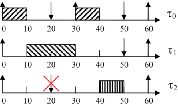
Let us consider the scenario 3 in which the value of the priority of the third tasks is greater than the other tasks. The following figure shows that the third task does not end its execution before its deadline. Thus, a classical scheduling method deduces that the system is not schedulable.
Figure 3: Pessimistic tasks executions 4.2. Proposed method
4.2.1. System information
First, we add the tasks to the representation of the system. The result is a universe PV-domain. Then we add the static parameters. Thus the static parameter representing the scheduler indicates a fixed priority scheduler. Finally, we add the information concerning the tasks parameters. The result is a PV-domain representing the system information:
(
) (
)
(
) (
)
K
K
∩
≥
∩
≤
∩
∩
=
∩
=
∩
=
5
4
0
0
2 2 0 0R
R
P
R
system
system
It is important to notice that the partial knowledge of the release time of the third instance is taken into account easily and without any approximation. Moreover, the unknown parameter (P2) is not a
problem.
At the end of this part, the PV-domain representing the system is reduced.
4.2.2. Determining and validating groups
In this part we create the groups of interactions and we validate them whenever necessary.
First, we create an empty group inheriting the properties of system information. Then, we try to add the first task instance which is the first instance of the first task (τ0,0) because
∀
τi,j,
r
0,0≤
r
i,j. Thisdoes not need to be validated because the deadline of the task instance τ0,0 is after the end of the group.
Then, we try to add “sure interactions”. The first instance of the second task corresponds because its release time is between the beginning and the end of the group. Thus, we add the instance τ1,0 to the
group. This group needs to be validated because the deadline of the first instance occurs before the end of the group. Thus, the behaviors of the group are computed. All the parameters of the tasks of the group are exactly known, that is why there is only one behavior. The behavior of the group can be graphically represented as follows:
Figure 3: Behavior of the first group
The group is schedulable, thus we add the next group.
The following group is composed of the second instance of the first task. The group 2 is schedulable because the absolute deadline of the instance is after the group.
The third group is composed of the first instance of the first task. The beginning of the group is not exactly known because it depends on the constraints of the release time of the third task. This group is schedulable because the deadline is sure to be after the end of the group. We can notice that priority of the third task does not modify the schedulability of the system.
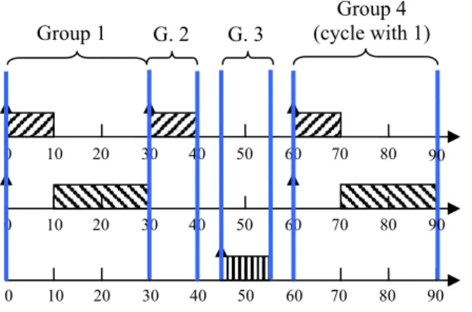
The next group is composed of the third instance of the first task and the second instance of the second task. This group is a cycle corresponding to the first group. Indeed, it is composed of the same tasks as the first group and the properties of the groups are the same. Thus, we do not validate this group and we do not compute its next group. All the groups have been computed; they are all schedulable, and thus the system is schedulable.
The following figure represents all the groups of the system and the cycle:
0 10 20 30 40 50 60 0 10 20 30 40 50 60
τ
0τ
1transitions
Group 1
τ
0τ
1τ
2 0 10 20 30 40 50 60 0 10 20 30 40 50 60 0 10 20 30 40 50 60Figure 4: All the groups of the system 4.3. Conclusion
By making hypotheses and approximations on the unknown or partially known tasks parameter, the classical method is pessimistic. On the other hand, the proposed method is well adapted to those problems and it is not pessimistic.
The validation of this system is a good example in which the pessimism of the classical methods like RMA induces an imprecise result indicating the unschedulability of the system. However, the system is schedulable and the proposed method proves it.
5. Conclusions
We propose a new non-pessimistic method to the analysis of real-time systems. This method can be used to represent systems with specific behaviors and complex relationships between their parameters, because any information that can be represented with a linear inequality can be taken into account. A major advantage of this method is that it can be used to validate a system at any design step. Indeed, this method can be used with partial knowledge and thus it is well adapted to reduce costs.
To complete this work, we intend to focus on two points: taking into account new system characteristics, and implementing a complete software. Indeed, several system behaviors have to be represented in our method (dependable and/or non-preemptive tasks, resources sharing, partitioning [17, 20]), which implies some modifications of the previously defined equations. We also plan to include specific components such as bounded buffers.
6. References
[1] R. Alur and al.: The algorithmic analysis of hybrid
systems, Theoretical Computer Science, 1995,
Volume 138, pages 3-34.
[2] R. Alur and al: Hybrid Automata: An Algorithmic
Approach to the Specification and Verification of Hybrid Systems, Hybrid Automata: An Algorithmic
Approach to the Specification and Verification of Hybrid Systems, 1992.
[3] R. Alur and al.: A theory of timed automata, Theoretical Computer Science, 1994, volume 126. [4] B. Andersson and J. Jonsson: Fixed-Priority
Preemptive Multiprocessor Scheduling: To Partition or not to Partition, Proceedings of the Int'l
Conf. on Real-Time Computing and Applications, 2000, IEEE Computer Society Press.
[5] R. Bagnara: A hierarchy of constraint systems for data-flow analysis of constraint logic-based languages, Science of Computer Programming,
1998.
[6] T. P. Baker: A stack-based resource allocation
policy for realtime, Real-Time Systems
Symposium, 1990, IEEE Computer Society Press. [7] L. P. Briand and D. M. Roy: Meeting Deadlines in
Hard Real-Time Systems: The Rate Monotonic Approach, 1999, IEEE Computer Society.
[8] Airlines Electronic Engineering Committee:
ARINC Specification 653, 1997.
[9] N. Halbwachs and Y-E. Proy and P. Raymond:
Verification of Linear Hybrid Systems by Means of Convex Approximations, Static Analysis
Symposium, 1994.
[10] T. A. Henzinger and P-H. Ho and H. Wong-Toi:
HyTech: The Next Generation, IEEE Real-Time
Systems Symposium, 1995.
[11] T. A. Henzinger and P-H. Ho and H. Wong-Toi: A
User Guide to HyTech, Tools and Algorithms for
Construction and Analysis of Systems, 1995. [12] T. A. Henzinger and P-H. Ho and H. Wong-Toi:
HYTECH: A Model Checker for Hybrid Systems,
International Journal on Software Tools for Technology Transfer, 1997.
[13] Thomas A. Henzinger and al.: What's decidable
about hybrid automata?, Proceedings of the 27th
Annual Symposium on Theory of Computing, 1995.
[14] Doran K.Wilde: A Library For Doing Polyhedral Operations, INRIA, 1993.
[15] Patrice Quinton, Sanjay Rajopadhye and Tanguy Risset: On manipulating Z-Polyhedra, IRISA, 1996.
[16] R. Bagnara, P. M. Hill, and E. Zaffanella:
Widening operators for powerset domains,
Quaderno 349, Dipartimento di Matematica, Università di Parma, Italy, 2004.
[17] J. Rushby: Partitioning in Avionics Architectures: Requirements, Mechanisms, and Assurance, SRI
International, Menlo Park USA, 1999.
[18] L. Sha and R. Rajkumar and J.P. Lehoczky:
Priority Inheritance Protocols: An Approach to
Real-Time Synchronization, IEEE Transactions on Computers, 1990.
[19] H. Le Verge: A Note on Cherniakova's algorithm, INRIA, 1992.
[20] B. L. Di Vito: A Formal Model of Partitionning for
Integrated Modular Avionics, NASA Langley
Research Center, 1998. 0 10 20 30 40 50 60 0 10 20 30 40 50 60 0 10 20 30 40 50 60 70 80 70 80 70 80 Group 1 Group 4 (cycle with 1) G. 2 G. 3 90 90 90