Computational tools for assembly oriented design

Computational Tools for Assembly Oriented Design

by

Stephen J. Rhee

B.S. Engineering and Applied Sciences California Institute of Technology, 1994

M.S. Mechanical Engineering

Massachusetts Institute of Technology, 1996

SUBMITTED TO THE DEPARTMENT OF MECHANICAL ENGINEERING IN PARTIAL FULFILLMENT OF THE

REQUIREMENTS FOR THE DEGREE OF MECHANICAL ENGINEER

at the

MASSACHUSETTS INSTITUTE OF TECHNOLOGY

September 1999

@ 1999 Massachusetts Institute of Technology All rights reserved

Signature of Author Db9nt of Mechanical Engineering August 23, 1999 Certified by Accepted b D iel E. Whitney Se * esearch Scientist Center for Technology, Policy, and Industrial Development Lecturer, Department of Mechanical Engineering Thes i sor

y

Ain A. Sonin Chairman, Departmental Committee on Graduate Students

TE y

Computational Tools for Assembly Oriented Design

by

Stephen J. Rhee

Submitted to the Department of Mechanical Engineering on August 23, 1999 in Partial Fulfillment of the Requirements for the Degree of Mechanical Engineer

ABSTRACT

It has been shown that it is necessary to consider manufacturing and assembly issues during the design phase of product development for numerous reasons. Doing so will allow for a better designed product in terms of ease and cost of manufacture and assembly in addition to a more robust product that best satisfies its intended functionality. It is the goal of assembly oriented design (AOD) methods to aid the designer in taking assembly issues into consideration during the design process to produce a design that can be better manufactured and assembled. The AOD methodology also allows for the analysis of existing designs in addition to being able to indicate possible areas of improvements in a design.

The goal of this research is to develop an integrated suite of computational tools for assembly oriented design. This involves first studying the flow of design information in the AOD approach. Then, a formal design process can be outlined. Previously developed theory and software tools and methods exist for conducting assembly oriented design. This includes the datum flow chain assembly model for use in the design of assemblies and software tools to generate geometric precedence constraints on assembly sequences

(SPAS), determine all feasible assembly sequences given such constraints (LSG),

interactively edit assembly sequences (EDIT), check for proper constraint of assemblies (MLA), and determine the tolerances for an assembly (Tolerance Analysis). The roles of these tools in the AOD process has been examined. A new software tool, the Assembly Designer, has been developed that incorporates the theory to promote this AOD approach, providing a designer an integrated environment in which to develop assembly designs with seamless interfaces with the other existing software tools. The development of additional software tools such as DFCPR, a tool that automatically generates the precedence constraints on assembly sequences that result from the selected datum flow chain model of an assembly, and the modification of existing tools such as SPAS and MLA (Constraint Analysis) were also necessary to facilitate the proper integration of the software and theory so as to guide a designer through the AOD process.

The design process was then applied to an actual assembly from industry making full use of the software tools and methods developed. This case study demonstrated the benefits of using the AOD approach and the abilities of the software tools.

Thesis Supervisor: Dr. Daniel E. Whitney Senior Research Scientist

Acknowledgments

First, I would like to thank my advisor, Dr. Daniel E. Whitney, for giving me the opportunity to conduct this research. I appreciate all the guidance he has offered me over the years, pertaining to research and other matters as well. I would also like to

acknowledge Dr. Thomas L. De Fazio, Dr. Krish Mantripragada, and Jeffrey D. Adams for all their valuable assistance to me in this research.

I would also like to show my appreciation to all the friends I have made during my

time at MIT. They may never know the impact they have made on my life, and I can only hope that I might have similarly affected them even if only in some small way. From them

I have learned many things that can only be learned outside of the classroom but no less

valuable in life. I would especially like to thank Sun for giving me all her support over the years.

Finally, I would like to thank my family for always being there for me. Their constant support and faith in me have made my studies possible.

This material is based upon work supported by the National Science Foundation under Grant No. DM1 9610163. Any opinions, findings, and conclusions or recommendations expressed in this material are those of the author and do not necessarily reflect the views of the National Science Foundation.

Contents

2.1 ASSEMBLY SEQUENCE ANALYSIS ... 17

2.1.1 Precedence Relation Generation ... 17

2.1.2 Assembly Sequence Representation ... 18

2.1.3 Assembly Sequence Evaluation ... 18

2.2 DATUM FLOW CHAIN ... 19

2.2.1 Concept ... ... 19

2.2.2 Definition and Properties ... 20

2.2.3 M ates and Contacts ... 20

2.3 CONSTRAINT ANALYSIS ... 21

2.3.1 Feature Library ... 21

2.3.2 Algorithm ... 22

2.4 S UMMARY ... 22

3. ASSEM BLY ORIENTED DESIGN ... 23

3.1 AOD APPROACH ... 23

3.2 DESIGN PROCESS ... 24

3.3 S UMMARY ... 27

4. SOFTW ARE IM PLEM ENTATION ... 29

4.1 S OFTWARE LAYOUT ... 29

4.2 ASSEMBLY D ESIGNER ... 31

4.2.1 Datum Flow Chain Design ... 32

4.2.2 Feature Selection ... 35

4.2.3 Precedence Relation Generation ... 38

4.2.4 Constraint Analysis ... 44

5. CASE STUDIES ... 51 5.1 THROTTLE BODY ... 51 5.2 S U M M A RY ... 63 6. CONCLUSIONS ... ... 65 6.1 C ONCLUSION S ... 65 6.2 F UTURE W ORK ... 65 BIBLIOGRAPHY ... 69 APPENDIX A ... 71 A .1 D F C P R ... 71

List of Figures

2.1 An example DFC ... 19

3.1 Top-down AOD approach ... 24

3.2 Design process flowchart ... 25

4.1 Software map ... 30

4.2 Assembly Designer main window ... 31

4.3 Add Part window ... 33

4.4 Edit Part window ... 34

4.5 Edit Liaison window ... 35

4.6 Add Feature window ... 36

4.7 Feature Coordinate Transform window ... 36

4.8 Feature Information window ... 37

4.9 Edit Feature window ... 38

4.10 Select Feature window ... 38

4.11 SPAS window ... 39

4.12 Prismatic peg in prismatic hole assembly and feature definition ... 41

4.13 Alternative DFC's for prismatic peg in hole assembly ... 41

4.14 EDIT window ... 45

4.15 Liaison graph of an assembly in graphical and matrix form ... 46

4.16 DFC of an assembly in graphical and matrix form ... 47

4.17 Alternative DFC for the assembly ... 49

4.18 Another alternative DFC ... 50

5.1 Throttle body assembled ... 51

5.2 Throttle body disassembled ... 52

5.3 Throttle body liaison diagram ... 52

5.4 Global coordinate frame shown on bore ... 53

5.5 Throttle body datum flow chain ... 54

5.6 Geometrically feasible assembly sequence graph ... 57

5.7 Revised throttle body DFC ... 59

5.8 Geometrically feasible assembly sequence graph for revised DFC ... 60

5.9 Assembly sequence graph for revised DFC ... 61

List of Tables

2.1 Feature types ... 21

4.1 Software tools and their functions ... 30

4.2 Filename extensions ... 32

4.3 Disassembly axis vectors ... 40

5.1 Throttle body features ... 55

CHAPTER 1

Introduction

1.1 Motivation

It has been shown that it is necessary to consider manufacturing and assembly issues during the design phase of product development for numerous reasons. Doing so will allow for a better designed product in terms of ease and cost of manufacture and assembly in addition to a more robust product that best satisfies its intended functionality. Traditionally, product development began with the design process where a design engineer or design team would be responsible for producing a detailed design from which a given product would be manufactured. This design process consists primarily of product specification, preliminary design, and detail design. After the design has been finalized, product development enters the manufacturing phase where it is up to the manufacturing engineer or team to determine how best to manufacture and assemble the given design. However, since the design has already been fixed, much of the freedom in how the product can be assembled has been removed, often leading to difficult and costly assembly. It is the goal of assembly oriented design (AOD) methods to aid the designer in taking assembly issues into consideration during the design process to produce a design that can be better manufactured. This is done by taking advantage of the freedoms that exist during the design phase to optimize the design for assembly. The AOD methodology also allows for the analysis of existing designs in addition to being able to indicate possible areas of

Past research, as detailed in Chapter 2, has resulted in theory, methods, and computational tools that support the top-down structure of the AOD methodology. However, as the research efforts were conducted by a number of individuals over a considerable period of time, there is a noted lack of integration in the methods and computational tools that have resulted.

1.2 Goal of Research

The ultimate goal of this research is to develop an integrated suite of computational tools for assembly oriented design. The first step in satisfying the goals of this research is to then study the design process itself and the steps involved in the design process. After having outlined the design process, it is then necessary to study the flow of design information in the AOD approach. Thus, the first goal of this research is to develop a model for the flow and analysis of design data that support the AOD framework. After having accomplished this, it is then possible to examine currently existing software tools and determine their roles in the design process making any necessary modifications in addition to developing new software tools that realize the theories and methods in the top-down AOD approach. The final step is to provide the designer an integrated user interface to the available software tools that aid in the AOD process. This involves the development of a front end design environment that interfaces with existing and newly developed software modules, as many of the existing software tools were developed independently and lack a coherent user interface.

1.3 Thesis Overview

Chapter 2 presents a brief review of previous research, including methods and computational tools, that provide the foundation for the integration and development of the computational tools for assembly oriented design in this research. Chapter 3 presents the

AOD process and the flow of information within. Chapter 4 discusses the actual software

implementation. Chapter 5 gives case studies of actual assemblies and the application of the software tools. Finally, Chapter 6 presents overall conclusions and suggested directions for future work.

CHAPTER

2

Prior Work

This chapter gives a brief overview of previous work which is the foundation upon which this research is based. Previous research has been categorized into three subject areas: Assembly Sequence Analysis (ASA), Datum Flow Chain (DFC), and Constraint Analysis.

2.1 Assembly Sequence Analysis

De Fazio and Whitney [1] describes Assembly Sequence Analysis (ASA) as the methodology in which all mechanically feasible sequences are first generated, then they are edited based on given criteria, and finally compared on an economic basis.

2.1.1

Precedence Relation Generation

Bourjault [2] originally used a graph of contacts or liaisons between parts named a "liaison diagram" to model an assembly where a node represents a part and an arc between nodes represent a connection between two parts. He then developed an algorithm that was capable of generating all possible assembly sequences based on a series of yes-no questions based on part mates. After receiving user-input answers to these questions, the computer would then generate a series of constraints referred to as precedence relations. The form of precedence relations used in this thesis is as follows:

Li & ... & L >= Lm & ... & Ln

which is read as all liaisons in the set of liaisons { Li, ..., Lj I must be completed previous to

or simultaneously with the completion of all liaisons in the set of liaisons { Lm, -., L }.

Subsequently, De Fazio and Whitney extended this method making it more efficient

by adding new rules to the automatic reasoning that resulted in less questions to be

answered by the user. Independent of this work, Homem De Mello [3] approached the task of precedence constraint generation using a different set of questions. Whipple [4] developed another method known as the "onion-skin" method for generating all valid assembly sequences on a process of questions that likens disassembly to the peeling of an onion. Baldwin [5] subsequently took these methods and incorporated them into a software tool called SPAS that generates the precedence relations by asking the necessary questions to the user.

2.1.2

Assembly Sequence Representation

After having determined the precedence relations required to generate all possible assembly sequences, it is necessary to represent the assembly sequences. In his assembly sequence generation software [6], Bourjault uses a parts tree to represent assembly sequences which is not compact but is easy to comprehend as it somewhat mimics a physical assembly line. Homem De Mello developed an And-Or Graph representation [7] to represent assembly sequences which is a compact representation but difficult to use to see how an assembly progresses. De Fazio and Whitney developed the Liaison Sequence Diagram based on a directed graph to offer a compact representation of assembly sequences that also offers more information on an assembly sequence's state by state progress.

Using the Liaison Sequence Diagram, Lui [8] developed a program, SED (Sequence Edit and Display) that would create the Liaison Sequence Diagram and allow for editing of the sequence diagram. Abell [9] expanded on this and Whipple's stability analysis creating a fully user interactive software tool, EDIT, for editing and evaluating assembly sequences.

2.2

Datum Flow Chain

Mantripragada and Whitney [10, 11] propose the concept of the Datum Flow Chain

(DFC) for assembly modeling and the design of assemblies as a method of capturing the

locational and dimensional constraint plan inherent in an assembly design. Figure 2.1 shows an example of a DFC. Fixt ure 7 Disk 6 ₂ 5 Bo re 3 Screws 14 Shaf t Figure 2.1 An example DFC 2.2.1 Concept

Assembly requirements can be identified from top level customer requirements down to the manufacture and assembly of individual parts using a method called Key Characteristics (KC's) [12, 13]. These KC's capture the top level customer requirements

assembly. Thus, the DFC is used to model a given assembly with the intent of fulfilling the requirements of the KC's of the assembly.

2.2.2

Definition and Properties

A DFC is an acyclic directed graph connective model of an assembly that defines

the relationships between parts represented as nodes in the graph. A DFC identifies the part mates that convey dimensional control and identifies the hierarchy that determines which parts or fixtures define the location of other parts. The graph representation of a

DFC is a subset of the liaison diagram where the arcs have direction indicating how a part

defines the location of another part and a weight or label that indicates the number of degrees of freedom that are located. Note that in Figure 2.1, the numbers associated with the arcs do not represent the number of degrees of freedom located but simply enumerate the arcs themselves.

There are several properties that result from the definition of the DFC. There can be only a single root part that only has outgoing arcs. In addition, loops or cycles are not allowed as this would mean that a part would essentially be defining its own location. Finally, in a properly constructed DFC, each part should be constrained in all 6 degrees of freedom, unless there are degrees of freedom that are left unconstrained for functional reasons.

2.2.3 Mates and Contacts

In addition to the "mates," represented by directed arcs, which transfer locational and dimensional constraint, there may be "contacts" between parts, represented by dashed lines, that transfer partial constraint or provide reinforcement without any locational constraint. This distinction implies that contacts between parts can not be established until the parts involved have been fully constrained by their mates.

2.3 Constraint Analysis

Often designers make constraint mistakes, where parts may be over-constrained or even under-constrained. Adams and Whitney [14, 15] have defined an algorithmic constraint analysis procedure making use of screw theory [16, 17] to examine combinations of elementary features in order to determine proper constraint of parts.

Feature Type Degrees of Freedom Constrained

Prismatic Peg / Prismatic Hole 6 X Y Z Tx Ty Tz

Plate Pin in Through Hole 5 X Y Z Tx Ty

Prismatic Peg / Prismatic Slot 5 X Z Tx Ty Tz

Plate Pin in Slotted Hole 4 X Z Tx Ty Round Peg / Prismatic Slot 4 X Z Tx Ty Round Peg / Through or Blind Hole 4 X Y Tx Ty

Threaded Joint 4 X Y Tx Ty

Elliptical Ball and Socket 4 X Y Z Tx

Plate-Plate Lap Joint 3 Z Tx Ty

Spherical Joint 3 X Y Z

Plate Pin in Oversize Hole 3 Z Tx Ty

Elliptical Ball in Cylindrical Trough 3 X Z Ty

Thin Rib / Plane Surface 2 Z Ty Ellipsoid on Plane Surface 2 Z Tx Spherical Ball in Cylindrical Trough 2 X Z

Peg in Slotted Hole 2 X Ty

Spheroid on Plane Surface 1 Z

Table 2.1 Feature types

2.3.1

Feature Library

Adams defines 17 types of assembly features as listed in Table 2.1 along with the degrees of freedom constrained in their nominal orientation. These 17 feature types are not meant to be a complete representation of all possible assembly features, but span the set of possible combinations of degree of freedom constraint of rigid body objects. These assembly features are modeled as kinematic joints allowing the use of a twistmatrix representation that describes the relative freedom in motion that a feature allows.

2.3.2

Algorithm

The constraint analysis algorithm determines whether a set of features acting on a part fully constrain that part. A wrenchmatrix reciprocal to a twistmatrix describes the set of forces and torques that can be transmitted by the joint described by the twistmatrix. First, the twistmatrices for each of the features acting on a part are concatenated into a single twistmatrix. Then, the reciprocal wrenchmatrix of the resulting single twistmatrix is calculated. This wrenchmatrix represents the logical intersection of the wrenchmatrices of the individual features. Thus, if this wrenchmatrix is not empty, each row of the matrix indicates that the features on the part are trying to constrain that same degree of freedom of that part, the definition of overconstraint. Adams has implemented this in the software tool, MLA.

2.4 Summary

In this chapter previously developed theory and software tools and methods that form the basis for the AOD process described in the next chapter have been presented. In addition, the modification and interfacing of these existing software tools and methods with newly developed software tools that will provide a designer with an integrated suite of software tools that aid in the AOD process is covered in Chapter 4.

CHAPTER 3

Assembly Oriented Design

In this chapter, the assembly oriented design (AOD) approach is discussed. The general design process is described, in addition to the flow of information during the design process.

3.1 AOD Approach

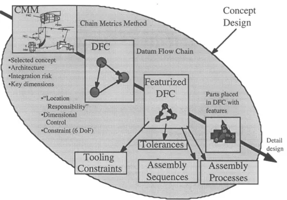
The AOD approach is a top-down design approach to modeling and analyzing assemblies and their assembly processes. The key goal of the AOD approach, as made obvious by its title, is to keep assembly issues in the foreground during the design process. As a result, it is desired that certain aspects of assembly analysis can be performed at an early stage when detailed part geometry may not be available. Thus, in this manner it is possible to examine how design changes affect the overall assembly. The end result should be an assembly design that satisfies both given design and assembly'requirements. Figure

3.1 gives a broad overview of the AOD approach. Initially, the design process begins with

concept design. A product architecture is defined from which Key Characteristics (KC's) can be extracted. These are then modeled into a datum flow chain (DFC) for the assembly design. Next, features can be attributed to the DFC that satisfy the dimensional control plan laid out by the DFC. Using this featurized DFC, assembly analyses such as generation of tolerances and assembly sequences can then be carried out during this design

... ... D etail

... design

Constraints

Assembly

Assembly

S

nces

Processes

Figure 3.1 Top-down AOD approach

3.2 Design Process

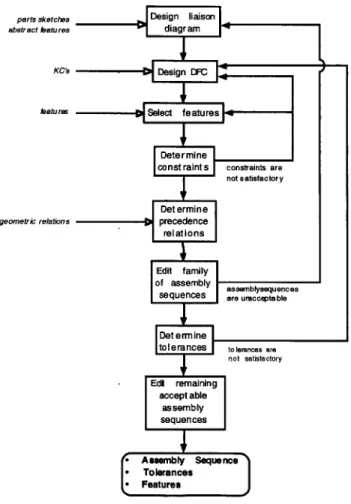
It is then necessary to outline a design process that follows the desired AOD approach. Figure 3.2 shows a flowchart for the design process as supported by the developed software tools and methods. This flowchart gives the nominal order of steps in the design process from beginning to end. However, the design process does not always follow such a linear order. Often, the design process is an iterative process where as more information becomes available, more details can be added to the design. This is critical to the idea of concurrent engineering where it is necessary to see how changes in different areas of the design affect the overall assembly. In addition, the design of an assembly may

not always start from scratch as much.of design that occurs in industry supports the idea of reuse where it is desirable that existing parts of previous designs are to be incorporated with some amount of redesign. Therefore, the starting point of the design process is not always predetermined as all the necessary information may not initially be available. Furthermore, it is often necessary to backtrack in the design process as new details of the design require changes in earlier parts of the design in order to support such changes. The loops in the flowchart are an attempt to capture these complexities of the design process. The incoming arrows from the left in Figure 3.2 show what information needs to be provided by the designer at each stage of the design process. All other information created during the design session by the designer and generated by the software tools flows down along the design process.

parts sketches Design liaison

abstract fatures diagram

KCs DC

fatures Select features

Dete r mine

const raint s constraints are

not satisfactory

Det ermine

geometric relations precedence

Initially, given some notion of the parts, e.g. parts sketches, and some notion of the connections between parts, a liaison diagram can be constructed. Then, using the key characteristics (KC's) of the assembly that need to be satisfied, a datum flow chain (DFC) can be determined. Next, specific features can be assigned to liaisons that satisfy the determined datum flow. Once having done this, the constraints of the assembly can be automatically generated. This will give information about whether certain parts are overconstrained, underconstrained, or sufficiently constrained. If these constraints are not satisfactory, it may be necessary to modify the design of the DFC or of the specific features. To generate the geometric precedence relations, more detailed information of the geometry of the parts is required. It is still not necessary to specify the exact geometries of the parts, but rather just the relations between parts and how they interfere with each other during assembly. In addition, precedence relations derived from the DFC are automatically generated. Using these precedence relations, the family of feasible assembly sequences is generated and can then be edited according to more specific criteria. If the resulting sequences are not satisfactory, it is necessary to backtrack in the design process. One may go back as far in the design process as one desires to affect changes in the possible assembly sequences. This is due to the fact that the precedence relations that limit the feasible assembly sequences come from both the geometries of the parts, of which features play a limiting role in determining escape directions and the liaisons between parts, and the datum flow chain, which is coupled with the design of the features. This tight coupling of the parts, the features, and the DFC is what makes it difficult to specify a linear sequence for the design process as significant changes in one may require the others to be modified to support such a change. After having determined that the remaining assembly sequences are satisfactory, the tolerances can be determined. This requires the building of the tolerance chain for the specific design which in large part is specified by the DFC. If the resulting tolerances are not satisfactory, it will be necessary to return to the design of the

examined to find an acceptable final assembly sequence. Thus, in the nominal flow of the design process, the designer starts with a rough notion of the parts and connections between parts in addition to the KC's of the assembly. During the design process, the details of the assembly become further specified, and at the end, the assembly sequence, the tolerances, and the features have all been specified. In the case that the designer wishes to redesign or perform an analysis on a existing design, it can be seen that the design process just begins with much of the design already specified and the existing process can still be applied.

3.3 Summary

In this chapter, the idea of the assembly oriented design approach has been presented. In addition, a design process, as formalized in flowchart format, that supports the AOD approach with the developed and existing software tools has been developed. This required the determination of what information must be presented by the user at each step in the design process in addition to what information can flow down from one step to the next. The next chapter will briefly present the previously existing software tools and describe in detail the newly developed software tools that support this AOD design approach.

CHAPTER 4

Software Implementation

This chapter presents the software tools developed that aid a designer through the

AOD process. In addition, the integration of the newly developed software tools with

existing software tools is discussed in detail. The Assembly Designer (AD) is the main software tool that provides the user a central front end to the AOD methodology in addition to the necessary interfaces with existing software tools and methods. The Datum Flow Chain Precedence Relation (DFCPR) module is a faceless background module that was developed to provide for the algorithmic generation of precedence relations from a datum flow chain.

4.1 Software Layout

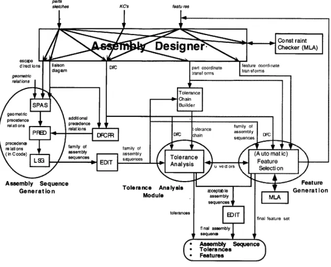
In Chapter 3, the flowchart of the design process in an AOD framework was presented. Figure 4.1 shows the layout and flow of the software tools that support the design process as given in Figure 3.2. In the software map, boxes represent software modules. Arrows between boxes represent the information that is passed between two software modules and the labels denote the exact data that is passed. Input arrows with italicized labels represent input from the user. The greyed out portions represent areas of future research that have not yet been implemented. Table 4.1 lists the major software tools and gives a brief description of each.

KCs featu res

Figure 4.1 Software map

Table 4.1 Software tools and their functions

pacs sketches

Software Module Function

Assembly Designer front end user interface for designing the DFC along

with selecting the features

Constraint Checker (MLA) checks for constraints given the DFC and the features

using constraint analysis

SPAS derives the geometric precedence relations through a

series of yes/no questions

DFCPR _{derives the precedence relations that result from the DFC} PRED translates the precedence relations into C code

LSG _{determines all feasible assembly sequences given the}

precedence

EDIT allows for interactive editing of sequences

4.2 Assembly Designer

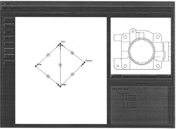
The Assembly Designer (AD) software tool presents a designer with an environment in which to design an assembly, including all the necessary interfaces to other software modules in order to provide the designer a seamless, integrated design session. The software was written in C++ using X1I and Motif libraries to handle the graphics and is currently running on a UNIX workstation. Figure 4.2 shows the main window of AD. The main window consists of a menubar, a toolbox, the Assembly Window, the Part Window for displaying parts, and the Text Window for general information.

Figure 4.2 Assembly Designer main window

Table 4.2 lists the file extensions that AD uses for importing and exporting data and a brief explanation of each file extension.

File Extension Description

.par names of parts along with part id numbers and graphical

r 7_ positions in the assembly window

.lia liaisons along with connected parts' id numbers and type

of connection (mate with dof's, contact, unspecified)

.ptr part coordinate transforms

.fea feature type, attributes, and coordinate transforms Sldn liaison diagram incidence matrix

.dfc datum flow chain incidence matrix

.ctf degrees of freedom (for dfc) incidence matrix

.adi liaison diagram adjacency matrix .ran part names

.ld liaison diagram (liaisons and names of connected parts) .rc_ escape directions for parts of each liaison

_pr geometric precedence relations

.prd datum flow chain precedence relations

.pra all precedence relations

Sin input to MLA (includes part coordinate transforms,

feature types, attributes, and coordinate transforms)

.zap feasible assembly sequences

.exp input to EDIT (includes part names and liaison diagram)

Table 4.2 Filename extensions

4.2.1

Datum Flow Chain Design

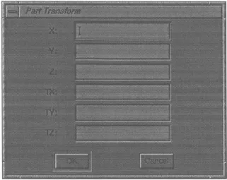
The design of a datum flow chain consists of three functional elements: parts, liaisons (which are specified as mates or contacts, or left unspecified in the intermediate stages of the design process), and features. The toolbar on the left of the Assembly Window, as can be seen in Figure 4.2, allows for the design and editing of DFC's with the following self-explanatory tools: Part, Liaison, Mate, Contact, Feature, Show, Edit, and Delete. The first step of the design process requires building a connective model of the assembly. Using the Part tool, the designer specifies nodes in the Assembly Window for each part. When a new part is created, the program asks the designer to enter a name for the part and the part coordinate transform from the global coordinate frame as shown in Figure 4.3. At this point, this information, especially the part coordinate transform, is

optional until later needed when checking for proper constraint of the assembly, which is discussed in section 4.2.4.

Figure 4.3 Add Part window

Now, the connections between parts can be modeled. This is done by using the Liaison tool. By clicking the pointer on a part and dragging to another part, the designer can specify liaisons between parts. Note that at this point, very little knowledge of the assembly needs to be known, i.e. what parts exist and what connections exist between parts. With only this initial information, it is possible to determine the geometric precedence relations as covered in section 4.2.3 and generate all geometrically feasible assembly sequences as shown in section 4.2.5.

The next step in building a DFC for an assembly is to decide which liaisons act as mates, and which act as contacts. Recall that mates provide locational constraint whereas contacts merely provide support. The Mate and Contact tools are used to specify each of the liaisons in the assembly. This can be done by selecting an existing liaison with either tool or using the tool to draw a new mate or contact between two parts as with the Liaison tool. A contact is represented graphically in the Assembly Window as a dashed line and a mate as an arrow. When specifying a liaison as a contact, no further information is

freedom are constrained in addition to selecting the proper direction in which that constraint is provided. The number of degrees of freedom constrained by a mate is shown graphically in the Assembly Window by a number next to the head of the arrow of the mate as can be seen in Figure 4.2. After completing the DFC, the precedence relations that are imposed by the DFC can be generated as shown in section 4.2.3 and covered in detail in

section 4.3. Now, the family of feasible assembly sequences that satisfy the constraints imposed by the DFC can be examined (see section 4.2.5).

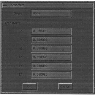
Figure 4.4 Edit Part window

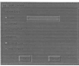
The DFC can also be edited and examined using the Show, Edit, and Delete tools. Using the Show tool, the designer can select a part or a liaison and have the part or parts connected by a liaison displayed in the Part Window if part drawings are available and textual information about the part or liaison displayed in the Text Window. The Edit tool allows the designer to change a part's name or modify the part coordinate transform of a part if a part is selected, as in Figure 4.4. If a liaison is selected, the designer can specify whether the liaison is a mate, contact, or unspecified, and if the liaison is a mate, modify

the number of degrees of freedom constrained and the direction of the mate, as shown in Figure 4.5.

Figure 4.5 Edit Liaison window

Finally, the Delete tool is used to remove unwanted parts or liaisons. In addition, if a part is deleted, all liaisons involving that part are also deleted.

4.2.2

Feature Selection

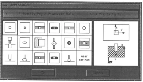
Once a DFC has been created to model an assembly, it is then necessary to specify the features on the parts that achieve the liaisons. This is done using the Feature tool. Selecting a liaison using the Feature- tool presents the designer with a feature selection window, as shown in Figure 4.6. The window presents the designer with icons for each of the 17 features listed in Table 4.1. When a feature is selected, a more detailed view of the feature is displayed along with the textual description from the table.

Figure 4.6 Add Feature window

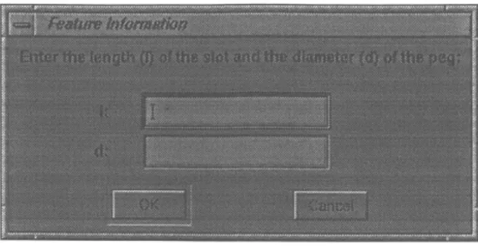
After the feature type is selected, the designer is prompted to enter the part to feature coordinate transform and also the specific attributes of the selected feature as shown in Figures 4.7 and 4.8.

Figure 4.8 Feature Information window

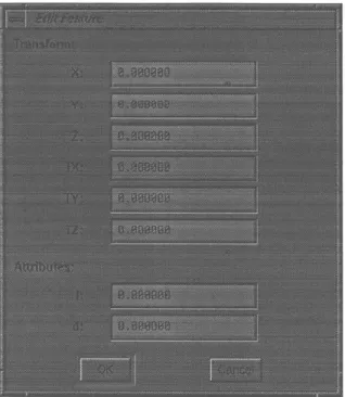
After a feature has been fully specified, it is displayed graphically on the liaison in the Assembly Window as a circle containing the letter 'f and a number. The number represents the number of features associated with that particular liaison. The Show, Edit, and Delete tools can also be used to edit and examine features. By selecting a feature with the Show tool, the parts connected by the feature are displayed in the Part Window, and the feature type, coordinate transform, and attributes are displayed in the Text Window. The Edit tool can be used to modify the coordinate transform and attributes of a feature as shown in Figure 4.9. If more than one feature exists, the designer is prompted to select which feature to modify among those present as seen in Figure 4.10. The Delete tool simply deletes a selected feature, and if more than one feature exists, again the designer is prompted for which feature to delete.

Figure 4.9 Edit Featurd window

Figure 4.10 Select Feature window

4.2.3

Precedence Relation Generation

Two types of precedence relations can be generated that impose constraints on the feasible assembly sequences for a given assembly. The first are those due to geometric interference and the second are those due to the theory of the datum flow chain. By using

for generating precedence relations, SPAS or DFCPR, and have the results displayed in the Text Window.

SPAS, originally written by Baldwin and given a new user interface by the author,

is used to generate geometric precedence relations. This is done by asking the designer a series of questions in order to determine the geometric interferences that exist as discussed in section 2.1.1. Figure 4.11 shows an example session with SPAS.

Figure 4.11 SPAS window

In addition, SPAS can use disassembly axis vectors, or escape directions, to automatically determine certain cases of geometric interference. If the designer has already attributed features onto the DFC of an assembly, escape directions are automatically generated and supplied to SPAS to reduce the amount of user input required in determining the geometric precedence relations. A disassembly axis vector is the vector along which a part must be moved in order to remove it from another part. Thus, the disassembly axis

involved in that liaison. For each of the 17 features in the feature library, Adams has defined the feature coordinate frames such that either disassembly (and thus assembly) must occur along the z-axis, or it may be ambiguous as there might exist multiple possible paths for disassembly. Using Adams' feature library, it is then possible to assign a disassembly axis to each feature; however, the direction of the disassembly axis vector for a part involved in that feature can be either positive or negative in the feature's coordinate frame as there are two parts, one which has an escape direction in the +z direction and the other in the -z direction. This problem can be solved by utilizing the definition of the base part in each of Adams' features. When the user enters the feature coordinate transform for a feature, the software asks for the coordinate transform relative to the coordinate frame of a part. This part is assumed to be the base part in the feature definition so that the disassembly axis vector for the base part associated with the feature can then be taken to be in the positive direction by the software when calculating the escape directions. Table 4.3 lists all 17 features and the disassembly axis vectors for the base parts of each feature. Note that a vector of (0, 0, 0) denotes that the disassembly axis vector is ambiguous.

Feature Type Disassembly Axis Vector

Prismatic Peg / Prismatic Hole (0, 0, 1)

Plate Pin in Through Hole (0, 0, 1)

Prismatic Peg / Prismatic Slot (0, 0, 0)

Plate Pin in Slotted Hole (0, 0, 1)

Round Peg / Prismatic Slot (0, 0, 0)

Round Peg / Through or Blind Hole (0, 0, 1)

Threaded Joint (0, 0, 1)

Elliptical Ball and Socket (0, 0, 1)

Plate-Plate Lap Joint (0, 0, 0)

Spherical Joint (0, 0, 1)

Plate Pin in Oversize Hole (0, 0, 1)

Elliptical Ball in Cylindrical Trough (0, 0, 0)

Thin Rib / Plane Surface (0, 0, 0)

Ellipsoid on Plane Surface (0, 0, 0)

Spherical Ball in Cylindrical Trough (0, 0, 0)

Peg in Slotted Hole (0, 0, 1)

B

z

(a) (b)

Figure 4.12 Prismatic peg in prismatic hole assembly and feature definition: (a) example two-part assembly and (b) the feature definition from the feature library that models the feature involved in the liaison between the two parts

B B

A eA

(a) (b)

Figure 4.13 Alternative DFC's for prismatic peg in hole assembly

Thus, the disassembly axis vectors listed in Table 4.3 are for the base part in Adams' feature definition. For example, consider the simple two-part assembly consisting of a prismatic peg (part A) in a prismatic hole (part B) and their respective part coordinate frames shown in Figure 4.12(a). The corresponding feature definition and the feature coordinate frame is shown in Figure 4.12(b). If given the DFC shown in Figure 4.13(a), part B is the source part in the DFC and the software will ask the user for the feature coordinate transform relative to part B's coordinate frame. As the prismatic hole is the base part in the feature definition, the software uses Table 4.3 correctly to determine that part B's disassembly axis vector is (0, 0, 1), i.e. +z direction, in the feature's coordinate frame.

However, consider if the DFC is as shown in Figure 4.13(b). Here, the source part in the

DFC is part A. However, according to the geometry of parts A and B, one might be

inclined to associate part A, the peg, with the peg in Adams' feature definition and hence give the feature to part A coordinate transform as a 180 degree rotation around the y-axis. However, this would be incorrect as it would map* part A's escape direction into the -z direction in its part coordinate frame. Since part A is the source part, it should be associated with the base part in the feature definition and the feature to part A coordinate transform should be the identity transform, such that the software can correctly identify its disassembly axis vector in the +z direction in the feature coordinate frame and hence +z direction in part A's coordinate frame. This is due to the fact that the software does not distinguish which part is the peg or hole, only which part is the base part in determining the disassembly axis vector.

In summary, only a disassembly axis can be associated to a feature definition, not the actual direction vector. However, the actual vector can be associated with the base part in the feature definition. In addition, the software has no knowledge of the actual feature geometry of the parts, e.g. which part has the peg and which has the hole. The software must then assume that the source part in the DFC is the base part in the feature definition. The software is then capable of accurately determining the disassembly axis vectors of each of the parts using the information from Table 4.3 provided that the user enters the feature to part transform correctly such that the source part in the DFC is associated with the base part in the feature definition regardless of the actual feature geometry on the parts as was seen with the example DFC in Figure 4.13(b).

It has been acknowledged that this may not be the most intuitive manner for the user to assign features to liaisons, i.e. to define the feature to part coordinate transform such that the base part from the feature definition is associated with the source part in the DFC disregarding the actual feature geometry on the parts. This method has been chosen so as to limit the amount of explicit geometric information the user has to provide and allow the

software to still be able to calculate the disassembly axis vectors. For example, it may be known that a certain feature is to be used to join two parts, e.g. peg and slot, but the actual feature geometry on the parts may not yet have been decided upon, e.g. which part has a peg and which has a slot. Yet, the disassembly axis vectors should still be able to be determined. The alternative approach then is to take as input from the user the explicit feature geometry and allow the user to input the feature to part coordinate transform such that the geometry from the feature definition matches the geometry of the features on the parts. For example, when assigning the peg and slot feature to a liaison between two parts, the user would also input which part has the peg. In this method, the software would not have to assume that the source part in the DFC is the base part in the feature definition, for it would now explicitly know according to the user input. The software would then be capable of correctly determining the disassembly axis vectors of each part given the feature to part coordinate transform that matches up the geometry of the feature definition to the geometry of the features on the parts.

Once the correct disassembly axis vectors are known for each feature, the disassembly axis vector of a part involved in a liaison with multiple features can be determined. That is, for each liaison, the disassembly axis vector for each part can then be automatically generated. This is done by taking the disassembly axis vector for each feature attributed to the liaison and using the feature coordinate transform and part coordinate transform to determine the vector in the global coordinate frame. Next, the vectors for all features are compared. If they are all identical, then the disassembly axis vector for that part and that liaison is simply that vector. Otherwise, the disassembly axis vector is taken to be uncertain.

DFCPR is used to automatically generate the precedence relations that result from constraints imposed by the datum flow chain upon the feasible assembly sequences. DFCPR is covered in detail in section 4.3.

4.2.4

Constraint Analysis

Once the DFC for an assembly has been created and features have been added, it is possible to check for proper constraint of the assembly. This is done by using the menubar to access the Constraint Analysis module. Constraint analysis is one of the functions of Adams' MLA software tool. The Assembly Designer bypasses MLA's text based user interface for entry of part coordinate transforms and feature selection (including feature type, coordinate transform, and attributes). Thus, AD is in effect providing a graphical user interface for feature selection and using MLA solely as a faceless background module to check for proper constraint. Results are returned in the Text Window of AD.

4.2.5

Assembly Sequence Editing

The final module in the menubar calls Abell's EDIT software tool. There are two options for running this module. The designer may wish to generate the complete tree of geometrically feasible assembly sequences using only the geometric precedence relations from SPAS or just the family of assembly sequences that result after imposing the constraints due to the datum flow chain. Figure 4.14 shows an example session with

Figure 4.14 EDIT window

4.3 Datum Flow Chain Precedence Relation

An assembly can be graphically represented as a liaison graph where nodes represent parts or subassemblies and liaisons represent contacts or mates between parts. This liaison graph can also be stored in a matrix to facilitate computer manipulation where rows represent parts and columns represent liaisons. This specific matrix is referred to as an incidence matrix. Figure 4.15 depicts the relation between graphical and matrix representation. To create this matrix, rows are created for all parts in the assembly. Then, for each liaison in numerically sequential order, a column is created with a '1' in the rows of the two parts the liaison connects and a 'O' otherwise. Thus, it follows that for each column there must be exactly two elements with a value of '1'. For example, liaison 7

connects parts S3 and AS. Therefore, in its column, there are '1's in the rows for S3 and

AS and 'O's elsewhere.

S3 ₇ AS FS PC S1-2 AS S3 FS S4-11 Figure 4.15 5 S4-11 1 2 3 1 1 1 1 0 0 0 1 0 0 0 1 0 0 0 0 0 0 Liaison graph of an 2 S1-2 -1 PC 4 5 6 7 8 1 1 0 0 0 0 0 1 0 0 0 0 1 1 0 0 0 0 1 1 1 0 0 0 1 0 1 0 0 0

assembly in graphical and matrix form

The datum flow chain (DFC) is graphically represented using an ordered liaison graph. An ordered liaison graph is similar to a liaison graph except that liaisons now have a direction from one node to another. The DFC can also be represented by a matrix similar to one used for a liaison graph. In order to capture the direction of a liaison, a '-l' is used to indicate that a liaison points to a part and a '1' is used to indicate that a liaison originates from a part. Thus, for a DFC matrix, every column must have exactly one '-1' element and one '1' element. Figure 4.16 illustrates the DFC and accompanying matrix representation. Dashed lines represent liaisons that are contacts and thus not part of the datum flow chain.

9

0

0 0 0

S3 ₇ FS 2 S1 -2 9 _'1 S4-11 5 PC 2 4 6 7 8 9 PC -1 -1 0 0 0 0 S1-2 0 0 -1 0 0 0 AS 1 0 1 -1 0 0 S3 0 0 0 1 1 0 FS 0 1 0 0 -1 1 S4-11 0 0 0 0 0 -1

Figure 4.16 DFC of an assembly in graphical and matrix form

A given DFC layout imposes assembly constraints in addition to those due to the

geometric relations between parts. According to Mantripragada, these constraints can be summarized by the following two rules:

1. There can be no subassemblies with only contacts between parts.

2. There can be no subassemblies with incompletely constrained parts.

These rules are referred to as the contact rule and the constraint rule, respectively. These statements can then be translated into a computer algorithm operating on the matrix forms of the DFC and liaison graph to allow for automatic generation of precedence relations similar to those generated from geometric interferences between parts. Given the two rules listed above, there are two types of precedence relations generated.

To eliminate the possibility of subassemblies with only contacts between parts (contact rule), the liaison graph matrix and the DFC matrix are compared to determine which liaisons are contacts. Then, for each contact, a precedence relation stating that all

mates in the DFC pointing to the parts the contact connects must be completed before the contact can be completed is generated. For example, in Figure 4.16, liaison 3 joining parts

PC and S3 is a contact. Incoming mates to parts PC and S3 include liaisons 2 and 4.

Thus, liaisons 2 and 4 must be completed prior to or simultaneous with liaison 3 (2 & 4

3). This type of precedence relation generation will. ensure that subassemblies with only

contacts between parts will not be allowed.

To ensure that subassemblies with incompletely constrained parts are not allowed (constraint rule), each row in the DFC matrix is examined one at a time. If a part (row) has more than one incoming mate (element with value '-l'), then all incoming mates must be simultaneously completed to ensure that the part be fully constrained when assembled. For example, looking at the first row of the DFC matrix in Figure 4.16, part PC has two incoming mates, liaisons 2 and 4. Thus, liaisons 2 and 4 must be completed simultaneously (2 4 and 4 2).

The following is the list of precedence relations generated for the datum flow chain given in Figure 4.16: 2 & 4 & 6 > 1 2 & 4 3 2&4&9 5 2 4 4 2

Note that the first three precedence relations satisfy the contact rule discussed above while the last two relations satisfy the constraint rule.

S3 ₇

FS _{1 2 S1-2}

9

S4-11 5 PC

Figure 4.17 Alternative DFC for the assembly

Figure 4.17 depicts an alternative DFC layout for the assembly shown in Figure 4.15. Its accompanying precedence relations are as follows:

3 & 7 2 3&8 4 1 6 6 1 5 9 9 5

Figure 4.18 depicts yet another alternative DFC layout with the following precedence relations:

1 & 2 6

2& 3 7

3 &4 8

4 & 5 9

For this particular DFC, all precedence relations generated are due to the contact rule to ensure that there are no subassemblies with only contacts.

S3 ₇ Id" - - -' AS FS 2 'S1-2 \4 9\-S4-11 5 PC

Figure 4.18 Another alternative DFC

4.4 Summary

In this chapter, an overview of the software tools was presented in addition to a detailed account of the two newly developed software tools, AD and DFCPR. In the next chapter, these tools will be applied to the AOD process of real assemblies.

CHAPTER

5

Case Studies

This chapter examines real assemblies using the developed software tools in an

AOD framework.

5.1 Throttle Body

In our original assembly model, fasteners have largely been ignored as they have been considered to be more a part of the assembly process than actual parts in the assembly itself. However, in examining the throttle body, shown assembled in Figure 5.1 and disassembled into component parts and subassemblies in Figure 5.2, it has been determined that taking fasteners into consideration as part of the assembly model can provide useful insight.

Shaft Disk

@ @ Screws Figure 5.2 Throttle body disassembled

Disk

Screws

Figure 5.3 Throttle body liaison diagram

First, it is necessary to build an assembly model of the throttle body. The assembly consists of four parts: bore, shaft, disk, and screws. The parts are entered into the Assembly Designer software along with the connections that exist between the parts to arrive at the liaison diagram shown in Figure 5.3. For each part, the coordinate transform

from the part coordinate frame to the global coordinate frame is simply the identity transform, i.e. all part coordinate frames are coincident with the global coordinate frame with the origin located in the center of the bore on the axis of the shaft. Figure 5.4 shows the global coordinate frame with respect to the bore.

00 Y

0

z x

Figure 5.4 Global coordinate frame shown on bore

Once the liaison diagram has been created for the assembly, the next step is to build the datum flow chain model of the assembly. This involves determining which liaisons act as mates and which act as contacts and deciding upon the number of degrees of freedom that each mate constrains. In this assembly, the bore acts as the base part for the entire assembly. It in turn locates both the shaft and the disk. However, the shaft is not fully constrained by the bore. The shaft is free move along its axis when inserted into the bore. The shaft's degree of freedom that allows it to rotate on its axis has been ignored in this model of the assembly and is thus considered fixed. Thus, the bore locates the shaft in 5 degrees of freedom, i.e. all those except translation along the x axis. The shaft fully locates the screws in all 6 degrees of freedom. Finally, the bore, shaft, and screws act together to fully constrain the disk in all 6 degrees of freedom. The bore locates the disk in the x and y direction. The shaft locates the disk in the z direction and constrains rotations around the x and y axes. Lastly, the screws fix the disk's rotation around the z axis.

Disk

Screws re

aft

Figure 5.5 Throttle body datum flow chain

Figure 5.5 shows the datum flow chain (DFC) for the throttle body assembly. Note that this DFC model of the assembly consists entirely of mates as there are no contacts. Now it is necessary to select the features that realize the mates in the DFC. The "prismatic peg/prismatic slot" feature is used to model the mate between the bore and the shaft in order to model the shaft's single degree of freedom of translation along its axis. The mate between the bore and the disk is modeled by the "spherical ball in cylindrical trough" feature as the bore is basically a cylindrical trough and the disk has the same degrees of freedom as a spherical ball in a cylindrical trough. The disk is mounted in a groove in the shaft with some clearance and thus the "plate pin in oversized hole" feature is used to model the mate. The mate representing the screws in the shaft is accurately modeled by using two "plate pin in through hole" features, one for each of the two screws. Note that this choice of features does not explicitly fully constrain the screws in all 6 degrees of freedom as each feature only constrains 5 degrees of freedom, i.e. all but rotation around the z-axis; however, Constraint Analysis will show that rotation around the z axis is properly constrained by the combination of the two features as it should be. The final mate between the screws and the disk is modeled using two "plate pin in oversize

hole" features, capturing the interaction between each of the individual screws and the disk. These feature choices are summarized in Table 5.1.

Part 1 Part 2 Feature Transform

(X Y Z O,

,

Bore Shaft Prismatic Peg / Prismatic Slot 0000090

Bore Disk Spherical Ball in Cylindrical Trough 0009000

Shaft Disk Plate Pin in Oversize Hole 000000

Shaft Screws Plate Pin in Through Hole -1.21 00000 Plate Pin in Through Hole 1.21 00000 Screws Disk Plate Pin in Oversize Hole -1.21 0 0 0 0 0

I Plate Pin in Oversize Hole 1.21 0 0 0 0 0

Table 5.1 Throttle body features

After having completed the feature selection, it is then possible to use Constraint Analysis to check for proper constraint. Constraint Analysis reports that the bore and screws are fully constrained but that the shaft and disk are not fully constrained. Examining the DFC, it can be seen that the shaft has only 5 degrees of freedom constrained

by the bore. In the actual assembly, the disk provides constraint in the final degree of

freedom, translation along the shaft's axis. However, in the DFC model, the shaft is already locating the disk in 3 degrees of freedom, and the definition of the DFC states that it must be an acyclic graph of the assembly, i.e. loops or cycles are not allowed; otherwise, a part may in effect be locating itself. However, in the case of the throttle body, the shaft is locating the disk in translation along the z axis and rotations around the x and y axes, and the disk is really locating the shaft in translation along the x axis forming a loop in the current concept of the DFC. Yet since the shaft is locating the disk in different degrees of freedom than those in which it is being located by the disk, the shaft is not locating itself in any degree of freedom. This should then be considered a valid locating scheme. This leads to the conclusion that a DFC may have to allow for cycles or loops in cases where the