A computational approach to the quantification of animal camouflage

(1)

A Computational Approach to the Quantification of Animal Camouflage by

Derya Akkaynak

B.S., Aerospace Engineering, Middle East Technical University, Ankara (2003)

M.S., Aeronautics and Astronautics, Massachusetts Institute of Technology (2005)

Submitted to the Department of Mechanical Engineering and the Joint Program in Applied Ocean Science and Engineering

in partial fulfillment of the requirements for the degree of

Doctor of Philosophy in Mechanical and Oceanographic Engineering at the

MA

MASSACHUSETTS INSTITUTE OF TECHNOLOGY

and the

WOODS HOLE OCEANOGRAPHIC INSTITUTION June, 2014

SSACHUSETTS INSTITUTE OF TECHNOLOGY

AUG 15 2014

LIBRARIES

The author hereby grants to MIT and WHOI permission to reproduce and to distribute publicly copies of this thesis document in whole or in part in any medium now known or hereafter created.

Auho...Signature

redacted

-Author ...

- ig n a u e r d c d

...

Joint Program in Oceanography/Applied Ocean Science and Engineering MIT/WHOI May 23, 2014 Certified by A + b

oignature

reaactie

Signat

Dr. Ruth E. Rosenholtz Thesis Supervisor, P al Research Scientist, MIT

ire

redacted

e y...

Professor Henrik Schmidt Chair, Joint Committee for Applied 04 incience and Engineering, MIT/WHOI

Signature redacted

Accepted by... ...

Professor David E. Hardt Graduate Officer, Department of Mechanical Engineering, MIT

(2)

(3)

A Computational Approach to the Quantification of Animal Camouflage by

Derya Akkaynak

Submitted to the Department of Mechanical Engineering and the Joint Program in Applied Ocean Science and Engineering on May 23, 2014, in partial fulfillment of the requirements for the degree of

Doctor of Philosophy in Mechanical and Oceanographic Engineering

Abstract

Evolutionary pressures have led to some astonishing camouflage strategies in the animal kingdom. Cephalopods like cuttlefish and octopus mastered a rather unique skill: they

can rapidly adapt the way their skin looks in color, texture and pattern, blending in with their backgrounds. Showing a general resemblance to a visual background is one of the many camouflage strategies used in nature. For animals like cuttlefish that can

dynamically change the way they look, we would like to be able to determine which camouflage strategy a given pattern serves. For example, does an inexact match to a particular background mean the animal has physiological limitations to the patterns it can

show, or is it employing a different camouflage strategy (e.g., disrupting its outline)? This thesis uses a computational and data-driven approach to quantify camouflage patterns of cuttlefish in terms of color and pattern. First, we assess the color match of

cuttlefish to the features in its natural background in the eyes of its predators. Then, we study overall body patterns to discover relationships and limitations between chromatic components. To facilitate repeatability of our work by others, we also explore ways for unbiased data acquisition using consumer cameras and conventional spectrometers, which are optical imaging instruments most commonly used in studies of animal

coloration and camouflage. This thesis makes the following contributions: (1) Proposes a methodology for scene-specific color calibration for the use of RGB cameras for accurate and consistent data acquisition. (2) Introduces an equation relating the numerical aperture and diameter of the optical fiber of a spectrometer to measurement distance and angle, quantifying the degree of spectral contamination. (3) Presents the first study assessing the color match of cuttlefish (S. officinalis) to its background using in situ spectrometry. (4) Develops a computational approach to pattern quantification using techniques from computer vision, image processing, statistics and pattern recognition; and introduces Cuttlefish 72x5, the first database of calibrated raw (linear) images of cuttlefish.

Thesis Supervisor: Ruth Rosenholtz Title: Principal Research Scientist

(4)

(5)

(6)

(7)

Acknowledgments

Earning a doctoral degree from MIT is no doubt special, but for me, the most valuable part of this journey was having worked with Ruth Rosenholtz. I must have looked like a wrinkled shirt when I showed up at her door. After reading the first draft of our first paper, she said: "Good, now add your research questions to the introduction". I remember thinking "What? I did all this work, now I have to come up with questions?" Without any criticism, judgment or impatience, she ironed every single wrinkle. She never tried to change me; on the contrary, accepted and appreciated everything about me -including some distracting interests I had- and gave me all the room I needed to grow. I am forever grateful. It was an honor to work with her.

If I am receiving the title "Doctor" with this thesis, my husband Elron Yellin needs to

receive "Angel" for enduring a very rocky six years. Not only did he have to manage me while I was constantly under stress, but he also put his life on hold so I could pursue my lifelong dream of becoming an oceanographer. Thank you, Elron.

Being affiliated with three research institutions, I made many amazing friends, which also meant I could rant three times about the same subject in one day. Justine Allen initially became my "bff' as a part the scenario we developed to escape Turkish Coast Guard in case we got caught diving in a no-dive zone. We never got caught but the rest of the scenario played out. Kendra Buresch and Kim Ulmer taught me life was too short to not to have an umbrella in my drink, and a drink by the beach Wednesdays at 4 PM made a good tradition. Lydia Mathger was an amazing mentor who taught me more than half of the skills I learned during my PhD. Having had so much in common, I am sad not to have worked more closely with Liese Siemann, but I loved hearing the stories of her albino hedgehog. George Bell, Robyn Crook and CC Chiao made our lab a fun and significantly more productive place. Last but not least, Roger Hanlon, of course, got me interested in applying to the MIT/WHOI Joint Program in the first place, and took me on many dive trips during which we chased cuttlefish and octopus with the strangest optical

instruments. Thanks to him, I even learned some biology, and punctuation.

Every stressed and moody grad student needs a younger brother to torture, and I was lucky Shaiyan Keshvari happened to be at the right place at the right time for me to do just that. With Lavanya Sharan and Erik Hemberg, I took full advantage of the athletics

studio in our building and worked my way up to a tripod headstand in a year. Krista Ehinger made the ultimate sacrifice a grad student can make: she selflessly gave up the desk with the window so I could have it. Phillip Isola spent countless hours showing me computer vision tricks but in turn he got to see exclusive photos of camouflaged

cuttlefish, which he was fascinated by, so I think we're even. When Bei Xiao moved away, my life was immediately 90% duller, but somehow I got more work done. MIT friends Alvin Raj, Nat Twareg, Jie Huang, Stella Jia, Wenzhen Yuan, Zhengdong Zhang and Honghua Chang and John Canfield all made me look forward to coming to the office every day, especially on Mondays when we had lab lunch and fun conversations. Rui Lui is the only international celebrity I have known in person. I must thank Prof. Ted Adelson separately; I am always inspired by his ability to explain complex concepts in simple,

(8)

easy-to-digest parts. During one lab lunch he said: "I don't like math, I don't like

programming, I don't like reading papers", and I thought that was very humbling coming from a scientist and inventor whose workds had been cited more than 30,000 times. At Coffee 0', on a stinky fishing boat in Alaska, "feeding the fish" over the Gulf Stream or surrounded by penguins in Antarctica, I have some unforgettable scenes in my head with oceanographer friends Clay Kunz, Chris Murphy, Jeff Kaeli, Geoff Gorman, Wu-Jung Lee, Heather Beem, Audrey Maertens, Kalina Gospodinova, Ankita Jain, Nick Loomis, Stephanie Petillo, Toby Schneider and Sheida Danesh. I am looking forward to making future memories.

I am thankful for the support I received from WHOI from Jim Preisig, Tim Stanton, Dana

Yoerger, Andy Bowen, Meg Tivey and Chris Reddy. Judy Fenwick, Julia Westwater, Valerie Caron, Marsha Gomes and Leanora Fraser were never tired of helping. At MIT, Ronni Scwartz and Leslie Regan gladly answered about fifty emails I sent per day. I wholeheartedly believe that the mechanical engineering department can keep its doors open thanks to Leslie. Lonny Lippsett gave me the inspiration (and the strategy) to write a paper in 7 days; thanks to him I had fun writing this thesis, too.

I would also like to thank my thesis committee members: John Leonard, Charlie Chubb, Aran Mooney and Norm Farr, for providing great feedback on my research and

encouragement along the way.

Finally, I thank my dad and my sister, for their love and support and always being there for me.

(9)

Chapter 1 Introduction

Evolutionary pressures have led to some astonishing camouflage strategies in the animal kingdom. One kind of spittlebug evolved to look like bird droppings. Some fish in Amazonian waters adopted the appearance of fallen leaves, and spend all daylight hours motionless on the riverbed (Stevens and Merilaita 2009). In the tropics, brightly colored wing patterns of many butterflies send warning signals to predators indicating that these prey are toxic and should not be consumed. Some of these butterflies are perfectly palatable; they are only mimicking the appearance of their toxic cousins who live nearby (Boggs et al. 2003). Cephalopods like cuttlefish and octopus, which lost their hard outer shell millions of years ago, now depend on camouflage for survival, and have mastered a rather unique skill: they can rapidly adapt the way their skin looks in color, texture and pattern, blending in with their visual backgrounds (Hanlon and Messenger 1996;

Messenger 200 lb) - a trait noted in Aristotle's Historia Animalium (Aristotle 1910), and grossly exaggerated in many Greek myths.

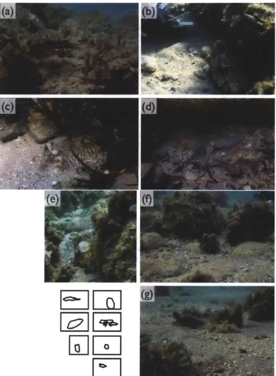
change their looks that makes cephalopod camouflage impressive; they match their surroundings in color and pattern without actually sensing color with their eyes (Mathger et al. 2006; Marshall and Messenger 1996). Figure 1.1 shows a small subset of the many different body patterns of cuttlefish we observed during the field season of 2011 in Urla, Turkey.

One immediately wonders their capabilities: "How many different

camouflage patterns can cuttlefish show?" "How well does one pattern camouflage the cuttlefish compared to another it could have shown?" "Does each of these

patterns fool a different aspect of the predator's visual system?" These are arguably the most important questions in the study of biological camouflage today, generalizing to animals other than

cuttlefish. We can best investigate such questions using a comprehensive approach that takes into account the properties of the natural environment camouflage is

displayed against, the ambient light field

But it is not only their ability to dynamically

What is camouflage?

There are many ways to camouflage without having a body pattern that exactly matches, or resembles a particular background. In biology, camouflage is an umbrella term that describes all strategies used for concealment, including body patterning and coloration, mimicking behavior, and motion (Stevens and Merilaita

2009). While there is no widespread consensus

on the definitions of camouflage in the biology community, they are often described based on

theirfunction or strategy: i.e. thefunction of

the evolutionary adaptation, such as breaking up form; as opposed to the strategy, the specific perceptual processes targeted, e.g. does the pattern disrupt normal edge detection mechanisms? In this thesis, we are most interested in the crypsis function, which aims to initially prevent detection and includes

strategies of background matching, distractive markings, disruptive coloration, self-shadow concealment, obliterative shading and flicker-fusion camouflage. Figure 1.2 shows examples of camouflage strategies associated with the crypsis function.

and the visual system of the observer(s) viewing the camouflage.

To interpret a scene with a camouflaged animal--in a laboratory setting or in the

wild--we would like to be able to describe the animal's camouflage quantitatively, so we can compare certain properties of its pattern to those of its environment. For example, we would like to be able to determine how closely the colors of the animal's body pattern

(14)

match the colors of its background. If we have a model representing the visual system of a predator, we might even be able to assess whether the animal's colors are

distinguishable from those of its background in the eyes of that predator. In the same way, we can investigate whether there are any similarities between the spatial

composition of a pattern (e.g., lines, splotches, dots, etc.) and the features found in its natural background. Two pre-conditions must be met before undertaking such

quantitative analyses. First, the data representing the camouflage scene must be acquired in an unbiased fashion, using the appropriate calibrated instrument(s). In the field of animal coloration and camouflage, most commonly used instruments for data acquisition are consumer cameras, conventional spectrometers and multi/hyper-spectral imagers. Second, the methodology used for pattern quantification must be objective, free of subjective input from human observers, to facilitate repeatability of work by other researchers.

In this thesis, we use a data-driven and computational approach to quantify camouflage patterns of European cuttlefish (Sepia officinalis) using techniques from computer vision, image processing, statistics and pattern recognition. For cuttlefish (and other cephalopods such as squid and octopus), the body pattern, describing the overall appearance of the animal at any given moment, consists of chromatic (e.g., light or dark), textural (e.g., smooth or rough), postural (e.g., skin papillae and arm postures) and locomotor (e.g., buried or hovering) components, all of which can be combined in many ways (Hanlon and Messenger 1996; Messenger 200 1b). The visual nature of cephalopod communication and their versatility have led to thinking of the production of body patterns as behaviors (Packard and Hochberg 1977) much like feeding, foraging,

reproduction and communication. We utilize images of camouflage scenes collected with both consumer cameras and conventional spectrometers. To ensure our analysis of camouflage meets the necessary pre-conditions mentioned above, we first explore ways of acquiring unbiased data using commercial-off-the-shelf cameras (Chapter 2) and conventional spectrometers (Chapter 3). Then, we investigate biologically important questions regarding cuttlefish camouflage. In Chapter 4, we present the first study that assesses color match of cuttlefish in the eyes of its predators, using spectral data collected

in situ. Quantifying the color matching abilities of cuttlefish is important because cuttlefish are colorblind (Marshall and Messenger 1996; Mathger et al. 2006). In

addition, the properties of ambient light that penetrates to cuttlefish habitats underwater generally makes all objects appear blue or green, except for those at very shallow depths

(Ahldn 2005; Jerlov 1976; Akkaynak et al. 2011; Smith and Baker 1978; Vasilescu

2009). What degree of color match is sufficient to fool the visual systems of predators in

such chromatically limited underwater environments?

After investigating color match, we move on to the analysis of entire body patterns of cuttlefish. This is a difficult problem because models of visual pattern perception for fish predators do not exist; and therefore we can only approach this problem from the point of view of the human visual system. Since cuttlefish can dynamically and rapidly change the way their body pattern looks, it is not always straightforward to determine which

camouflage strategy their pattern might serve. If they do not display a good resemblance to their backgrounds, is it because they are using a different camouflage strategy (e.g., disruptive coloration, see Figure 1.2), or because they have physiological limitations that prevent them from generating a pattern with a good match to that background? We

(15)

investigate the camouflage pattern generating capabilities of cuttlefish from calibrated photographs in Chapter 5. Understanding limitations to the patterns cuttlefish show can give us insights into determining whether cuttlefish are capable of employing more than one camouflage strategy. Even though it has not been experimentally proven for

cephalopods, Hanlon and colleagues present evidence of disruptive coloration in two different species of cuttlefish (Hanlon et al. 2009; Hanlon et al. 2013). If cuttlefish can indeed employ different camouflage strategies, when we investigate the structure of the space their patterns form, we might expect to observe well-separated, discrete number of clusters, instead of a continuum. Such analyses can contribute to the ongoing research regarding how many camouflage patterns cuttlefish can show, and in turn, help answer how many total camouflage patterns there may be in all of animal kingdom.

Imaging camouflage patterns

The tools used to study camouflage, particularly to image animals and their backgrounds are important because the appearance of a camouflage scene may be different when viewed by a non-human animal's visual system. Indeed, our lack of consideration or knowledge of the visual mechanisms of the relevant observers is thought to be one of the major obstacles hindering full understanding of camouflage strategies (Stevens and Merilaita 2009). We know less about the visual systems of animals than we do about humans' (Stevens et al. 2007; Mathger et al. 2008), but taking into account the visual capabilities of the observer(s) viewing a camouflage pattern is important because analyzing color signals from the point-of-view of humans and making inferences about their appearances to animals often produces erroneous conclusions. This is because animal visual systems differ from ours in important ways. For example, birds have four photoreceptors, one more than humans with normal color vision. In addition, they are sensitive to the ultraviolet (UV) part of the electromagnetic spectrum (Hart et al. 1998), to which we are not. In a recent publication, Stoddard and Stevens (Stoddard and Stevens

2011) showed that some common cuckoo eggs (which are laid in nests of other species

and often hatched and raised by unsuspecting host birds) appeared to have a good color match to the host eggs when viewed by humans, but had clear and quantifiable

differences when modeled in avian color space. Their study highlights a key point: the optical instrument that will be used to image camouflage pattern must be capable of recording information in the parts of the electromagnetic spectrum to which relevant observers are sensitive.

Three kinds of optical instruments are used for imaging animal patterns: consumer cameras (also known as RGB cameras), spectrometers and hyper-spectral imagers (Akkaynak 2014). Among these, hyper-spectral imagers provide the most comprehensive data because in addition to recording a spatial image, they also densely sample the electromagnetic spectrum, creating an image of dimensions Nx Mx P. These dimensions correspond to height (N), width (M) and the number of spectral samples (P, typically between 70-100). Despite being ideal instruments for imaging animal patterns in

color, hyper-spectral imagers are least commonly used for animal coloration studies because of their high cost and physical bulkiness. In addition, their slow imaging times that make it difficult to photograph moving objects like animals in the wild. Consumer

(16)

hyper-spectral imagers because they also do spatial imaging; however they are limited in color capture capabilities.

Figure 1.1 The versatility of cuttlefish, and its remarkable ability to combine pigments with textural elements and body postures makes these animals perfect models for the study of camouflage. Here we show a subset of body patterns, used for communication and camouflage, that we observed in cuttlefish's (S.officinalis) natural habitat on the Aegean coast of Turkey. Image credits: Derya Akkaynak, Justine J. Allen & Roger T. Hanlon.

(17)

By design, consumer cameras sample the electromagnetic spectrum narrowly,

creating images of dimensions Nx Mx 3, and the parts of the spectrum they record data from are chosen to overlap with the sensitivities of the human visual system (Akkaynak et al. 2014; Stevens et al. 2007). Even when it is desired or acceptable to capture a photograph just in the visible range, there are a number of manual processing steps required before camera-dependent colors can be transformed into a camera-independent color space, which is a minimum requirement to facilitate repeatability of work by others in the context of scientific applications. In the field of animal coloration and camouflage, the limitations of consumer cameras and the need to manually process their images were generally overlooked until the work of Stevens et al. (2007), who emphasized that in-camera processed photographs (e.g., images injpg format) may contain artifacts that cannot be removed, compromising data quality. In this work, we expand their study that focused on consistency of colors captured with consumer cameras, and introduce a method to also increase the accuracy of color capture using consumer cameras. We call this method scene-specific color calibration, and describe it in detail in Chapter 2.

To overcome the color limitations of consumer cameras, conventional spectrometers with optical fibers are frequently used in their place, or in tandem, to measure colors from an animal's habitat, nest, eggs, body parts, skin, fur and plumage (Akkaynak 2014). Spectrometers sample the electromagnetic spectrum densely with the capability to record information outside of the visible range. However, the image they record is a single pixel big (i.e., has dimensions 1 x 1 x P), requiring multiple

measurements on a carefully gridded setup, and a complex reconstruction scheme to capture spectra for the entire layout of a pattern. In addition, depending on the optical properties of a fiber, it may not be possible to resolve spectra from features that are very small without colors from neighboring features mixing in. For features that are large enough, recording uncontaminated spectra demands the positioning of the optical fiber as close as possible to surface being measured, without touching it. This is standard practice in laboratory setups but not easily accomplished in field studies because it is challenging to get the fiber very close to freely behaving animals in the wild. In Chapter 3, we

investigate what kinds of camouflage assessment errors contaminated spectra can lead to if the surveyor fails to get very close to the feature being measured.

Quantifying camouflage patterns

Given a camouflage pattern, we would like to be able to determine which aspects of the visual background it may match, or which camouflage strategy it serves. This is not straightforward because quantitative models describing camouflage strategies do not exist. Mathger and colleagues (2008) were to first to quantitatively analyze the color matching abilities of cuttlefish. They measured reflectance spectra from ten points on animals and background substrates in the laboratory and used normalized Euclidean distance to quantify spectral difference. They found that cuttlefish showed a better spectral match to natural substrates than they did for artificial substrates, but did not analyze the discriminability of colors according to the visual systems of predators. Chiao and colleagues (2011) also performed a color match assessment in the laboratory, but they used a hyper-spectral imager to capture body patterns. They modeled the visual systems of hypothetical predators and found that the colors cuttlefish produced were indistinguishable in the eyes of predators. In both studies, the natural substrates used

(18)

were sands and gravel. Cuttlefish live in habitats ranging from the Mediterranean to the coral reefs of West Africa, which have a diversity of background substrates that extend beyond sands and gravel including three-dimensional elements like sea grass, pinna, rocks, boulders, etc. We advanced existing work by travelling to one of the natural habitats of cuttlefish in the Aegean Sea and conducting the first in situ spectroscopic survey of color and luminance from cuttlefish skin and substrates from that habitat. Then, we calculated color and luminance contrast using the Vorobyev-Osario receptor noise model (Vorobyev and Osorio 1998), which allowed us to assess the discriminability of colors in the eyes of hypothetical di- and tri-chromat predators (Chapter 4). In this field study, we focused only on quantifying spectral discriminability, omitting spatial

configurations of body patterns, which we investigate in Chapter 5.

To compare one camouflage pattern with another and quantify the differences between them, it is important to use a dataset that is free of instrument bias, and an analysis method that does not contain subjective judgments. To facilitate repeatability of our work by others, prior to our analysis of overall camouflage patterns, we created Cuttlefish72x5, the first database consisting of linear images of camouflaged cuttlefish. It was important to establish this database before asking biological camouflage questions because previous work describing animal patterns and coloration often based their

analyses on images injpg format. Such images are standard outputs of consumer cameras and have been processed and compressed in ways that they no longer maintain a linear relationship to scene radiance (Stevens et al. 2007; Akkaynak et al. 2014). This means that they may not accurately represent the pattern that was photographed. In addition,

earlier studies that describe camouflage patterns involved subjective judgments by human observers. While assessments of patterns by human observers is quick and does not require any specialized instruments, it is inherently subjective and the resulting

qualitative descriptions often vary between observers, causing low repeatability (Stevens

2011). Thus, camera bias and processing artifacts were minimized for the images in our

database, facilitating repeatability of our results by other researchers. Based on the images in the Cuttlefsh72x5 database, we focused on three aspects of cuttlefish camouflage patterns and used computational methods to investigate them: the relationship between the level of expression of components in terms of intensity and mottleness; the structure of the camouflage pattern space (e.g., do patterns form discrete clusters or a continuum), and whether cuttlefish can show all of the patterns they are theoretically capable of producing. These questions are investigated in detail in Chapter

(19)

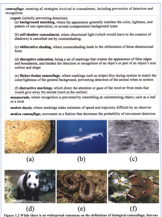
camouflage, meaning all strategies involved in concealment, including prevention of detection and

recognition

crypuis (initially preventing detection):

(a) background matching, where the appearance generally matches the color, lightness, and pattern of one (specialist), or several (compromise) background types

(b) self-shadow concealment, where directional light (which would leave to the creation of

shadows) is cancelled out by countershading.

(c) obliterative shading, where countershading leads to the obliteration of three-dimensional

form

(d) disruptive coloration, being a set of markings that creates the appearance of false edges

and boundaries, and hinders the detection or recognition of an objet's or part of an object's true outline and shape

(e) flicker-fusion camouflage, where markings such as stripes blur during motion to match the color/lightness of the general background, preventing detection of the animal when in motion

(f) distractive markings, which direct the attention or gaze of the receiver from traits that

would give away the animal (such as the outline)

masquerade, where recognition is prevented by resembling an uninteresting object, such as a leaf

or a stick

modon dazzle, where markings make estimates of speed and trajectory difficult by an observer

modon camouflage, movement in a fashion that decreases the probability of movement detection

(a)

(b)

(c)

(d)

(e)

()

Figure 1.2 While there is no widespread consensus on the definitions of biological camouflage, Stevens and Merilaita (2009) provide the most comprehensive set of descriptions, which we adopt in this work. (a) Background matching by cuttlefish (b) Counter-shaded grey reef shark (c) Obliterative shading makes one of the two decoy ducks in this photograph disappear (on the right, practically invisible) while the non-countershaded on the left is visible (d) Disruptive pattern of a panda bear (e)

The patterning of the common European viper might trigger a flicker-fusion illusion (f) False eye spots serve as distractive markings on this brush-footed butterfly. Image credits: (a): Hanlon Lab,

(20)

Chapter 2 Unbiased data acquisition: Commercial-off-the-shelf digital

camerasi

2.1 Introduction

State-of-the-art hardware, built-in photo enhancement software, waterproof housings and affordable prices enable widespread use of commercial off-the-shelf

(COTS) digital cameras in research laboratories. However it is often overlooked that

these cameras are not optimized for accurate color capture, but rather for producing photographs that will appear pleasing to the human eye when viewed on small gamut and low dynamic range consumer devices (Chakrabarti et al. 2009; Seon Joo et al. 2012). As such, use of cameras as black-box systems for scientific data acquisition, without

knowledge and control of how photographs are manipulated inside, may compromise data quality and in turn, hinder repeatability. For example, a common color-sensitive use of consumer cameras is in the field of animal coloration and camouflage (Stevens et al.

2007; Pike 2011 b). How well do the colors from the skin of a camouflaged animal match

the colors in a particular background? For an objective analysis of this question, the photograph of the animal taken by a researcher using a certain make and model COTS

camera should be reproducible by another researcher using a different camera. This is not straightforward to accomplish because each camera records colors differently, based on the material properties of its sensor, and built-in images processing algorithms are often make and model specific, and proprietary. Thus, for scientific research, manual

processing of COTS camera images to obtain device-independent photographs is crucial. In this chapter, we explore the following question: what are the pre- and post-image acquisition steps necessary so color capture using COTS cameras is consistent and accurate enough to yield photographs that can be used as scientific data? Our goal is to identify the limitations of COTS cameras for color imaging and streamline the manual processing steps necessary for their use as consistent and accurate scientific data acquisition instruments.

A consumer camera

photograph is considered raw image iiage

unbiased if it has a known (linear RGB)

relationship to scene camera-speciic onversion nt

proprietary standard RG8 lossy

radiance. This can be a image processing space compression

purely linear relationship, (non-linear) (nonlinear)

or a non-linear one where Figure 2.1 Basic image-processing pipeline in a consumer camera. the non-linearities are

precisely known and can be I

inverted. A linear relationship to scene radiance makes it possible to obtain device-independent photographs that can be quantitatively compared with no knowledge of the original imaging system. Raw photographs recorded by many cameras have this desired property (Chakrabarti et al. 2009), whereas camera-processed images, most commonly

1 Parts of this chapter were previously published. See (Akkaynak et al. 2014) for full reference.

(21)

images injpg format, do not. For scientific research, obtaining device-independent photographs is crucial because each consumer camera records colors differently. Only after camera-dependent colors are transformed to a standard, camera-independent color space, researchers using different makes and/or models of cameras can reproduce them.

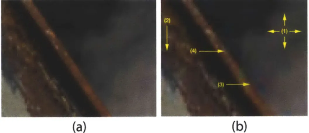
When pixel intensities in photographs are to be used as scientific data, it is important to use raw images, and manually process them, controlling each step, rather than using camera-processed images. In-camera processing introduces non-linearities through make and model-specific and often proprietary operations that alter the color, contrast and white balance of images. These images are then transformed to a non-linear RGB space, and compressed in an irreversible fashion (Figure 2.1). Compression, for instance, creates artifacts that can be so unnatural that they may be mistaken for cases of image tampering (Figure 2.2) (Farid 2011). As a consequence, pixel intensities in

consumer camera photographs are modified such that they are no longer linearly related to scene radiance. Models that approximate raw (linear) RGB from non-linear RGB images (e.g., sRGB) exist, but at their current stage they require a series of training images taken under different settings and light conditions as well as ground-truth raw images (Seon Joo et al. 2012).

(a)

(b)

Figure 2.2 (a) An uncompressed image. (b) Artifacts after jpg compression: 1) grid-like pattern along block boundaries 2) blurring due to quantization 3) color artifacts 4) jagged object boundaries. Photo credit: Dr. Hany Farid. Used with permission.

(22)

2.2 Background and related work

The limitations and merit of COTS cameras for scientific applications have previously been explored, albeit disjointly, in ecology (Levin et al. 2005), environmental sciences (De La Barrera and Smith 2009), systematics (McKay 2013), animal coloration (Stevens et al. 2007), dentistry (Wee et al. 2006) and underwater imaging (Ahldn 2005; Akkaynak et al. 2011). Stevens et al. (Stevens et al. 2007) wrote:

"... most current applications of digital photography to studies of animal coloration fail to utilize the full potential of the technology; more commonly, they yield data that are qualitative at best and uninterpretable at worst".

Our goal is to address this issue and make COTS cameras accessible to

researchers from all disciplines as proper data collection instruments. We focus on two aspects of color capture using consumer cameras: consistency (Ch. 2.3-2.7) and accuracy

(Ch. 2.8). Calibration of consumer cameras through imaging photographic calibration

targets (i.e., camera characterization) is a technique well known to recreational and professional photographers for obtaining consistent colors under a given light source. Researchers in fields like image processing, computer vision and computational

photography also frequently use this technique (Szeliski 2010; Shirley et al. 2009; Pharr and Humphreys 2010; Joshi and Jensen 2004). However, in the field of animal coloration, the limitations of consumer cameras and the need to manually calibrate them were

generally overlooked until the work of Stevens et al. (2007), who emphasized that in-camera processed photographs (e.g., images injpg format) may contain artifacts that cannot be removed, compromising data quality. In the first part of this chapter, we review and streamline the necessary manual processing steps described by Stevens et al. (2007) and others.

In Chapter 2.8, we introduce the idea of scene-specific color calibration and show that it improves color transformation accuracy when a non-ordinary scene is

photographed. We define an ordinary scene as one that has colors that are within the gamut of a commercially available color calibration target. Color transformation, which we describe in detail in Chapter 2.7, is done through a transformation matrix that maps device-specific colors to a standard, device-independent space based on known,

manufacturer-specified chromatic properties of calibration target patches. This

transformation matrix is generally computed through solving a system of equations with using linear least squares regression. Previous work that focused on increasing color transformation accuracy used standard, off-the-shelf calibration targets and investigated methods other than linear least squares regression to minimize the error between captured and desired RGB values. Examples of methods used include non-linear regression

(Westland and Ripamonti 2004), constrained least squares regression (Finlayson and Drew 1997), neural networks (Cheung et al. 2004) and interpolation (Johnson 1996). Our approach differs from existing work in that we use the simplest mathematical solution to the system of equations that describe the color transformation (i.e., linear least squares regression), and derive the desired set of RGB value directly from features in the scene instead of commercial photographic calibration targets.

Even though our work is motivated by accurate capture of colors from

(23)

science consumer cameras are used; we demonstrate this in Chapter 2.9 using real scientific problems. Throughout this work, "camera" will refer to "COTS digital cameras", also known as "consumer," "digital still," "trichromatic" or "RGB" cameras. Any references to RGB will mean "linear RGB" and non-linear RGB images or color spaces will be explicitly specified as such.

2.3 Color imaging with COTS cameras

Color vision in humans (and other animals) is used to distinguish objects and

surfaces based on record linear image (camera raw)

their spectral _include_calibration _{record spectra}

properties. Normal utarget in scene R from scene

human vision is

trichromatic; the -- demosaic section 2.8

retina has three cone _{apply white balance} _{section 2.C}

photoreceptors

pefrredetos suse calibration use ambient light

referred to as short (S, target OR setu

peak 440 nm),.ar OR spectrum

medium (M, peak 545 apply color transformation

nm) and long (L, peak

..

use calibration use spectra from

580 nm). Multiple target OR scene

light stimuli with section 2.D section 3.0

different spectral Figure 2.3 The workflow proposed for processing raw images. Consumer shapes evoke the cameras can be used for scientific data acquisition if images are captured

p . in raw format and processed manually so that they maintain a linear

same response. This relationship to scene radiance.

response is

represented by three

scalars known as tri-stimulus values, and stimuli that have the same tri-stimulus values create the same color perception (Wyszecki and Stiles 2000). Typical cameras are also designed to be trichromatic; they use color filter arrays on their sensors to filter

broadband light in the visible part of the electromagnetic spectrum in regions humans perceive as red (R), green (G) and blue (B). These filters are characterized by their

spectral sensitivity curves, unique to every make and model (Figure 2.4). This means that two different cameras record different RGB values for the same scene.

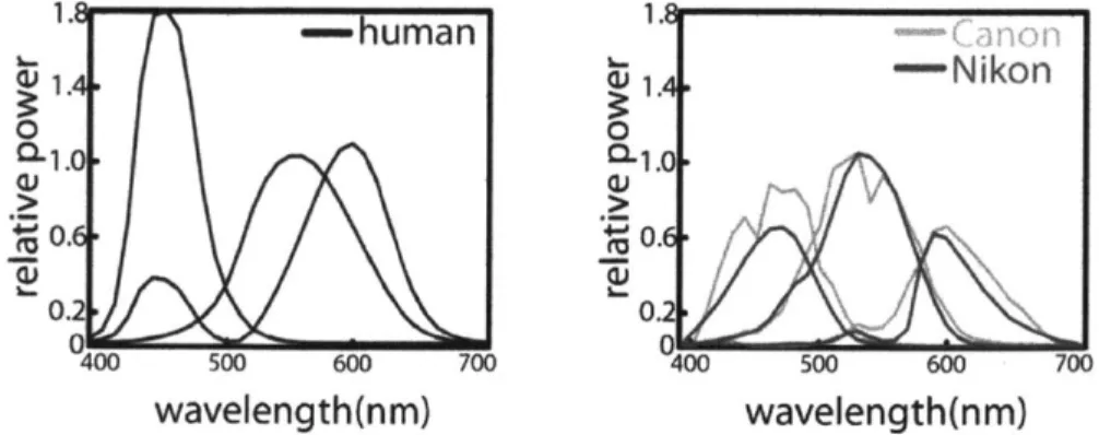
Human photoreceptor spectral sensitivities are often modeled by the color matching functions defined for the 2* observer (foveal vision) in the CIE 1931 XYZ color space. Any color space that has a well-documented relationship to XYZ is called device-independent (Reinhard et al. 2008). Conversion of device-dependent camera colors to device-independent color spaces is the key for repeatability of work by others; we describe this conversion in Ch. 2.7 & 2.8.

2.4 Image formation principles

The intensity of light recorded at a sensor pixel is a function of the light that illuminates the object of interest (irradiance, Figure 2.5), the light that is reflected from the object towards the sensor (radiance), the spectral sensitivity of the sensor and optics of the imaging system:

(24)

IC = k(y)cosO f"' S(X)Li(X)F(A, 6)dA. (2.1) Here c is the color channel (e.g., R, G, B), Sc (A) is the spectral sensitivity of that channel, Li (A) is the irradiance, F(A, 6) is the bi-directional reflectance distribution function and Amin and Amax _{denote the lower and upper bounds of the spectrum of}

interest, respectively (Szeliski 2010). Scene radiance is given by:

Lr (A) = Li(A)F (A,6) cos6, (2.2)

where F(A, 6) is dependent on the incident light direction as well as the camera viewing angle where 6 = (6, 4i, Or, r). The function k(y) depends on optics and other imaging parameters and the cos6; term accounts for the changes in the exposed area as the angle between surface normal and illumination direction changes. Digital imaging devices use different optics and sensors to capture scene radiance according to these principles (Table 1).

Table 1 Comparison of basic properties of color imaging devices

Device Spatial Spectral Image Size Cost Spectrometer x 1 x p > $2,000 COTS camera / x n x m x 3 > $200 Hyperspectral _{n x m x p} > $20,000 imager

2.5 Demosaicing

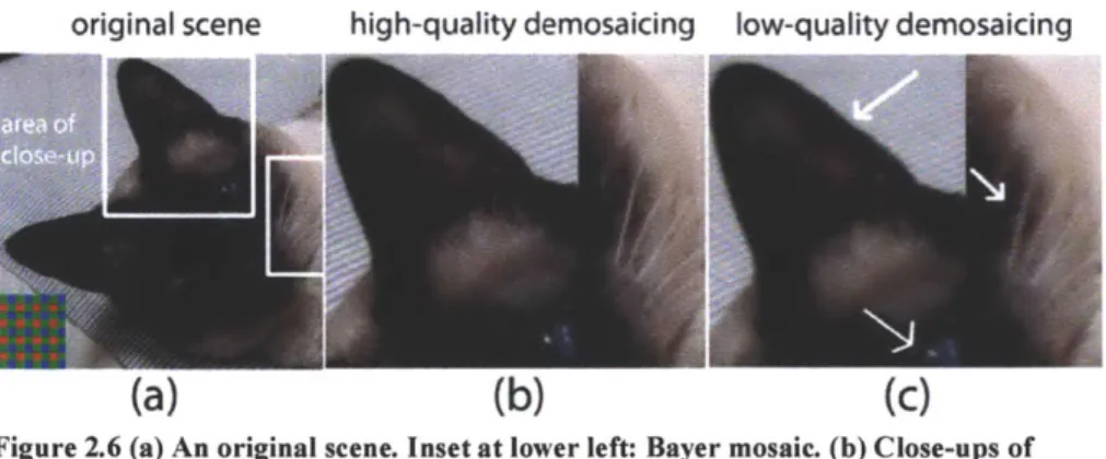
In single-sensor cameras the raw image is a two dimensional array (Figure 2.6a, inset). At each pixel, it contains intensity values that belong to one of R, G or B channels according to the mosaic layout of the filter array. Bayer Pattern is the most commonly used mosaic. At each location, the two missing intensities are estimated through

interpolation in a process called demosaicing (Ramanath et al. 2002). The highest quality demosaicing algorithm available should be used regardless of its computation speed (Figure 2.6), because speed is only prohibitive when demosaicing is carried out using the limited resources in a camera, not when it is done by a computer.

-human 1. - Nikon 0 0 c-c. 0. 0.2 400 500 600 700 0_7 500 600 700 wavelength(nm) wavelength(nm)

Figure 2.4 Human color matching functions for the CIE XYZ color space for 2* observer and spectral sensitivities of two cameras; Canon EOS iDs mk 11 and Nikon D70.

(25)

2.6 White

balancing

In visual perception and color reproduction, white has a privileged status (Finlayson and Drew 1997). This is because through a process called chromatic adaptation our visual system is able to discount small changes in the color of an

illuminant, effectively causing different lighting conditions to appear "white" (Reinhard et al. 2008). For example, a white slate viewed underwater would still be perceived as white by a SCUBA diver, even though the color of the ambient light is likely to be blue or green, as long as the diver is adapted to the light source. Cameras cannot adapt like humans, and therefore cannot discount the color of the ambient light. Thus, photographs must be white balanced to appear realistic to a human observer. White balancing often refers to two concepts that are related but not identical: RGB equalization and chromatic adaptation transform (CAT), described below.

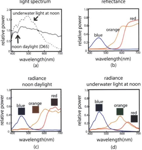
light spectrum reflectance

underwater light at noon

noon daylight (D65) 40 500 60 wavelength(nm) (a) radiance noon daylight Uri 106 0.8 0 0.2 > 0.4 *4-~0.2 re orang -blue t 0 4L 700 wavelength(nm) 500 600 wavelength(nm) (b) 700 radiance

underwater light at noon

1. ₁ 0 .4-0 Co 0. 0.4 0.2 04 ₅₀₀ ₆₀₀ ₇₀₀ wavelength(nm) (c) (d)

Figure 2.5 (a) Irradiance of daylight at noon (CIE D65 illuminant) and noon daylight

on a sunny day recorded at 3 meters depth in the Aegean Sea. (b) Reflectance spectra

of blue, orange and red patches from a Macbeth ColorChecker. Reflectance is the

ratio of reflected light to incoming light at each wavelength and it is a physical property of a surface, unaffected by the ambient light field, unlike radiance. (c) Radiance of the same patches under noon daylight on land and (d) underwater.

In scientific imaging, consistent capture of scenes often has more practical importance than capturing them with high perceptual accuracy. White balancing as

'I 1.5 0 CL a) 1.0 ..0.5 0.8 red bNueorje 0 0. 0.4 0.2 0 blue orange red U 1.U0 0 0 I

(26)

described here is a linear operation modifies photos so they appear "natural" to us. For purely computational applications in which human perception does not play a role, and therefore a natural look is not necessary, white balancing can be done using RGB

Equalization, which has less perceptual relevance than CAT, but is simpler to implement (see examples in Ch. 2.9). Here, we describe both methods of white balancing and leave it up to the reader to decide which method to use.

2.6.1 Chromatic Adaptation Transform (CAT)

Also called white point conversion, CAT models approximate the chromatic adaptation phenomenon in humans, and have the general form:

'PDIPs 0 0

Vd~eination = [MA

H

YDYs 0

][MA

]Vsource (2.3)

0 0 flD/fls

where VXYZ denotes the 3 x N matrix of colors in XYZ space, whose appearance is to be

transformed from the source illuminant (S) to the destination illuminant (D); MA is a 3 x3 matrix defined uniquely for the CAT model and p, y and 3 represent the tri-stimulus values in the cone response domain and are computed as follows:

P

Y = [MA] [WP]Yz i = S,D (2.4)

Here, WP is a 3x 1 vector corresponding to the white point of the light source. The most

commonly used CAT models are Von Kries, Bradford, Sharp and CMCCAT2000. The MA matrices for these models can be found in (SUsstrunk et al. 2000).

original scene high-quality demosaicing low-quality demosaicing

(a)(b)

(c)

Figure 2.6 (a) An original scene. Inset at lower left: Bayer mosaic. (b) Close-ups of marked areas after high-quality (adaptive) and (c) after low-quality (non-adaptive) demosaicing. Artifacts shown here are zippering on the sides of the ear and false colors

near the white pixels of the whiskers and the eye.

2.6.2 RGB Equalization

RGB equalization, often termed the "wrong von Kries model" (Westland and Ripamonti 2004), effectively ensures that the R,G and B values recorded for a gray calibration target are equal to each other. For a pixel p in the ith color channel of a linear image, RGB equalization is performed as:

(27)

WB pi-DSi _i = R, G, B _(2.5)

WSi- DSi

where p YB is the intensity of the resulting white balanced pixel in the ith channel, and

DS and WSi are the values of the dark standard and the white standard in the ith

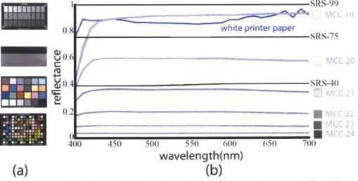
channel, respectively. The dark standard is usually the black patch in a calibration target, and the white standard is a gray patch with uniform reflectance spectrum (often, the white patch). A gray photographic target (Figure 2.7) is an approximation to a Lambertian surface (one that appears equally bright from any angle of view) and has a uniformly distributed reflectance spectrum. On such a surface the RGB values recorded by a camera are expected to be equal; but this is almost never the case due to a combination of camera sensor imperfections and spectral properties of the light field (Westland and Ripamonti 2004); RGB equalization compensates for that.

SRS-99

(1

f

white printer paper

a)

L.6 _SRS-40)

400 450 500 550 600 650 700

wavelength(nm)

(a)

(b)

Figure 2.7 (a) Examples of photographic calibration targets. Top to bottom: Sekonik

Exposure Profile Target 11, Digital Kolor Kard, Macbeth ColorChecker (MCC), ColorChecker Digital. (b) Reflectance spectra (400-700nm) of SpectralonTM targets

(black curves, prefixed with SRS-), gray patches of the MCC (purple), and a white sheet of printer paper (blue). Note that MCC 23 has a flatter spectrum than the white patch (MCC 19). The printer paper is bright and reflects most of the light, but it does not do so uniformly at each wavelength.

2.7 Color transformation

Two different cameras record different RGB values for the same scene due to differences in color sensitivity. This is true even for cameras of the same make and model (Stevens et al. 2007). Thus, the goal of applying a color transformation is to minimize this difference by converting device-specific colors to a standard, device-independent

space (Figure 2.8). Such color transformations are constructed by imaging calibration targets. Standard calibration targets contain patches of colors that are carefully selected to provide a basis to the majority of natural reflectance spectra. A transformation matrix T between camera color space and a device-independent color space is computed as a linear

least squares regression problem:

(28)

Here, Vgxroyznd truth and VGBr are 3 x N matrices where N is the number of patches in the calibration target. The ground truth XYZ tri-stimulus values Vg'rozund truth can either

be the published values specific to that chart, or they could be calculated from measured spectra (Ch. 2.7). The RGB values Vinear are obtained from the linear RGB image of the calibration target. Note that the published XYZ values for color chart patches can be used only for the illuminants that were used to construct them (e.g., CIE illuminants D50 or

D65); for other illuminants a white point conversion (Eq. 2.3&2.4) should first be

performed on linear RGB images.

before color transformation after color transformation (device-dependent colors) (device-independent colors)

0 _{6.ground truth} 0 >, . 0 Canon 0 o NIkon E% A Eiko :L1 . 0. .U 0. 7 7 U' 0.o u. U 0

chromaticity

x

chromaticity x

Figure 2.8 Chromaticity of Macbeth ColorChecker patches captured by two cameras, whose sensitivities are given in Fig. 5 in device-dependent and independent color spaces.

The 3 x 3 transformation matrix T (see (Westland and Ripamonti 2004) for other polynomial models) is then estimated from Eq. 2.6:

T = Vgroun trut2 Win3ear +

where the superscript + denotes the Moore-Penrose pseudo-inverse of the matrix V This transformation T is then applied to a white-balanced novel image Igear:

f orretd= TIine~r (28)

to obtain the color-corrected image Icozected, which is the linear, device-independent version of the raw camera output. The resulting image I'2 _{frected needs to be converted to}

RGB before it can be displayed on a monitor. There are many RGB spaces and one that can represent as many colors as possible should be preferred for computations (e.g., Adobe wide gamut) but when displayed, the image will eventually be shown within the boundaries of the monitor's gamut.

In Eq. 2.6, we did not specify the value of N, the number of patches used to derive the matrix T. Commercially available color targets vary in the number of patches they

have, ranging between tens and hundreds. In general, higher number of patches used does

(29)

and Finlayson 2008) found that 13 of the 24 patches of a Macbeth ColorChecker (MCC) are sufficient for most transformations. Intuitively, using patches whose radiance spectra span the subspace of those in the scene yields the most accurate transforms; we

demonstrate this in Figure 2.10. Given a scene that consists of a photograph of a MCC taken under daylight, we derive T using an increasing number of patches (1-24 at a time) and compare the total color transformation error in each case. We use the same image of the MCC for training and testing because this simple case provides a lower bound on error. We quantify total error using:

e = N ZL₁V(Li - LGT)2 + (A - AGT) 2 + (Bi - BGT)2 (2.9)

where an LAB triplet is the representation of an XYZ triplet in the CIE LAB color space (which is perceptually uniform); i indicates each of the N patches in the MCC and GT is

2 101 patch order 1 IMIr, r7 HWrmm

OW .. patch order 2 r mmene irmi

patch order 3

4-0

2 4 6 8 10 12 14 16 18 20 22 24

# of patches used in color transformation

Figure 2.9 Using more patches for a color transformation does not guarantee increased transformation accuracy. In this example, color transformation error is computed after 1-24 patches are used. There were many possible ways the patches could have been selected, only three are shown here. Regardless of patch ordering, overall color transformation error is minimized after the inclusion of the 18th patch. First six patches of orders 1 and 2 are chromatic and for order 3, they are achromatic. The errors associated with order 3 are higher initially because the scene,

which consists of a photo of a Macbeth ColorChecker, is mostly chromatic. Note that it is not

possible to have the total error be identically zero even in this simple example due to numerical error and noise.

the ground-truth value for the corresponding patch. Initially, the total error depends on the ordering of the color patches. Since it would not be possible to simulate 24! (6.2045 x

1023) different ways the patches could be ordered, we computed error for three cases (see

Figure 2.9 legend). Initial error is the highest for patch order 3 because the first six patches of this ordering are the achromatic and this transformation does poorly for the

MCC, which is composed of mostly chromatic patches. Patch orderings 1 and 2 on the

other hand, start with chromatic patches and the corresponding initial errors are roughly an order of magnitude lower. Regardless of patch ordering, the total error is minimized

(30)

2.8 Scene-specific color calibration (SSCC)

In Ch. 2.7, we outlined the process for building a 3x3 matrix T that transforms colors from a camera color space to the standard CIE XYZ color space. It is apparent from this process that the calibration results are heavily dependent on the choice of the

calibration target, or

the specific patches used. Then, we can hypothesize that if we had a calibration target that contained all the colors found

in a given scene, Urla, Turkey Woods Hole, MA Kona, HI USA

and only those Figure 2.10 Features from three different dive sites that could be used for scene-specific color calibration. This image first appeared in the December colors, we would 2012 issue of Sea Technology magazine.

obtain a color II

transformation with minimum error. In other words, if the colors used to derive the transformation T were also the colors used to evaluate calibration performance, the resulting error would be minimal - this is the goal of scene-specific color calibration.

The color signal that reaches the eye, or camera sensor, is the product of

reflectance and irradiance (Figure 2.5), i.e. radiance (Eq. 2. 1&2.2). Therefore, how well a calibration target represents a scene depends on both the chromatic composition of the features in the scene (reflectance) and the ambient light profile (irradiance). For example, a scene viewed under daylight will appear monochromatic if it only contains different shades of a single hue, even though daylight is a broadband light source. Similarly, a scene consisting of an MCC will appear monochromatic when viewed under a narrow-band light source even though the MCC patches contain many different hues.

Consumer cameras carry out color transformations from camera-dependent color spaces (i.e. raw image) to camera-independent color spaces assuming that a scene consists of reflectances similar to those in a standard color target, and that the ambient light is broadband (e.g., daylight or one of common indoor illuminants), because most scenes photographed by consumer cameras have these properties. We call scenes that can be represented by the patches of a standard calibration target ordinary. Non-ordinary

scenes, on the other hand, have features whose reflectances are not spanned by

calibration target patches (e.g. in a forest there may be many shades of greens and browns that common calibration targets do not represent), or are viewed under unusual lighting (e.g. under monochromatic light). In the context of scientific imaging non-ordinary

scenes may be encountered often; we give examples in Ch 2.9.

For accurate capture of colors in a non-ordinary scene, a color calibration target specific to that scene is built. This is not a physical target that is placed in the scene as described in Ch. 2.7; instead, it is a matrix containing tri-stimulus values of features from that scene. Tri-stimulus values are obtained from the radiance spectra measured from

features in the scene. In Figure 2.10 we show features from three different underwater habitats from which spectra, and in turn tri-stimulus values, can be obtained.

Spectra are converted into tri-stimulus values as follows (Reinhard et al. 2008):

(31)

where X1 = X, X2 = Y, X3 = Z, and K = Ty Ej. Here, i is the index of the wavelength

steps at which data were recorded, Ri is the reflectance spectrum and Ej the spectrum of irradiance; Y- are the values of the CIE 1931 color matching functions x, y, z at the ith wavelength step, respectively.

0 Dfloral samples 6C .... _{Macbeth ColorChecker} - Scene-specific color calibration

o I . -underwater light at noon

a i Macbeth patches

0

nond y.6t 4

-0 0 6 e " 50 100 150

chromaticity x # of floral sample

(a) (b)

FRED floral samples _{Macbeth ColorChecker} _{Scene-specific color calibration}

noon daylight

1

s]Macbeth patches nondylight 2 avraestl, es orSSC 1 21

chromatcty x 0# of floral sample 100 ab s

(c) (d)

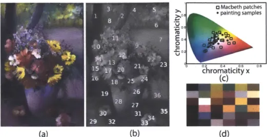
Figure 2.11 Scene-specific color transformation improves accuracy. (a) A "non-ordinary" scene

that has no chromaticity overlap with the patches in the calibration target (b) Mean error after scene-specific color calibration (arCC) is significantly less than after using a calibration chart. (c) An "ordinary" scene in which MCC patches span the chromaticities in the scene. (d)

Resulting error between the MCC and scene-specific color transformation is comparable, but on average, still less for hwCC.

Following the calculation of the XYZ tn-stimulus values, Eq. 2.6-2.8 can be used as described in Ch. 2.7 to perform color transformation. However, for every feature in a scene whose XYZ values are calculated, a corresponding RUB triplet that represents the camera color space is needed. These can be obtained in two ways: by photographing the features at the time of spectral data collection, or by simulating the RGB values using the spectral sensitivity curves of the camera (if they are known) and ambient light profile. Eq. 2. 10 can be used to obtain the camera RUB values by substituting the camera spectral sensitivity curves instead of the color matching functions. In some cases, this approach is more practical than taking photographs of the scene features (e.g., under field conditions when light may be varying rapidly), however spectral sensitivity of camera sensors is proprietary and not made available by most manufacturers. Manual measurements can be done through the use of a monochromator (Nakamura 2005), a set of narrowband

interference filters (Mauer and Wueller 2009), or empirically (Finlayson et al. 1998; Hong et al. 2001; Barnard and Funt 2002; Cheung et al. 2005; Jiang et al. 2013).

(32)

2.8.1 Scene-specific color calibration for non-ordinary scenes

To create a non-ordinary scene, we used 292 natural reflectance spectra randomly selected from a floral reflectance database (Arnold et al. 2010), and simulated their radiance with the underwater light profile at noon shown in Figure 2.11 a (scene 1). While this seems like an unlikely combination, it allows for the simulation of chromaticity coordinates (Figure 2.11 a, black dots) that are vastly different than those corresponding to an MCC under noon daylight (Figure 2.11 a, black squares), using naturally occurring light and reflectances. We randomly chose 50% of the floral samples to be in the training set for SSCC, and used the other 50% as a novel scene for testing. When this novel scene is transformed using an MCC, the mean error according to Eq. 2.9 was 23.8 and with

SSCC, it was 1.56 (just noticeable difference threshold is 1). We repeated this

transformation 100 times to ensure test and training sets were balanced and found that the mean error values remained similar. Note that the resulting low error with SSCC is not due to the high number of floral samples used (146) in training for SSCC, compared to only 24 patches in a MCC. Repeating this analysis with a training set of only 24 randomly selected floral samples did not change results significantly.

2.8.2 Scene-specific color calibration for ordinary scenes

We used the same spectra from scene 1 to build an ordinary scene (scene 2), i.e. a scene in which the radiance of the floral samples (Figure 2.11 c, black dots) are spanned

by the radiance of the patches of an MCC (Figure 2.11 c, black squares). In this case, the

average color transformation error using an MCC was reduced to 2.3; but it was higher than the error obtained using SSCC (Figure 2.11 d), which was 1.73 when 24 patches were used for training, and 1.5 with 146 patches.

Table 2 Summary of post-processing steps for raw images

# Camera, Light Demosaic White balance Color transformation

Sony A700, Incandescent indoor 4th gray & black in None -analysis in the

light Adobe DNG MCC camera color space

converter _{Eq. 5}

Canon EOS lDs Mark I, Version 6.3.0.79 _{MCC and SSCC}

Daylight (for list of other

Canon Rebel T2, Low-pressure raw image White point of None -analysis in the

I_ sodium light decoders, see ambient light camera color space

IV http://www.cyber spectrum

Canon EOS iDs Mark II, com.net/-dcoffin/ Eq. 5&10 SSCC

Daylight _dcraw/)

Canon EOS 5D Mark II, Daylight 4th gray& black in

A computational approach to the quantification of animal camouflage

AUG 15 2014

LIBRARIES

redacted

- ig n a u e r d c d

...

oignature

reaactie

Signat

ire

redacted

Signature redacted

Abstract

Acknowledgments

Contents

Chapter 1

Introduction

(a)

(b)

(c)

(d)

(e)

()

Chapter 2

Unbiased data acquisition: Commercial-off-the-shelf digital

camerasi

2.1

Introduction

(a)

(b)

2.2

Background and related work

2.3

Color imaging with COTS cameras

..

2.4

Image formation principles

2.5

Demosaicing

2.6

White

balancing

H

][MA

(a)(b)

(c)

f

(a)

(b)

chromaticity

chromaticity x

2.8

Scene-specific color calibration (SSCC)

1