HAL Id: lirmm-00371485
https://hal-lirmm.ccsd.cnrs.fr/lirmm-00371485
Submitted on 28 Mar 2009
HAL is a multi-disciplinary open access archive for the deposit and dissemination of sci-entific research documents, whether they are pub-lished or not. The documents may come from teaching and research institutions in France or abroad, or from public or private research centers.
L’archive ouverte pluridisciplinaire HAL, est destinée au dépôt et à la diffusion de documents scientifiques de niveau recherche, publiés ou non, émanant des établissements d’enseignement et de recherche français ou étrangers, des laboratoires publics ou privés.
The Structure of Level-k Phylogenetic Networks
Philippe Gambette, Vincent Berry, Christophe Paul
To cite this version:
Philippe Gambette, Vincent Berry, Christophe Paul. The Structure of Level-k Phylogenetic Networks. CPM: Combinatorial Pattern Matching, Jun 2009, Lille, France. pp.289-300, �10.1007/978-3-642-02441-2_26�. �lirmm-00371485�
The Structure of Level-k Phylogenetic Networks
Philippe Gambette, Vincent Berry, Christophe Paul
D´epartement informatique, L.I.R.M.M., C.N.R.S. - Universit´e Montpellier II. {gambette,vberry,paul}@lirmm.fr
Abstract. Evolution is usually described as a phylogenetic tree, but due to some exchange of genetic material, it can be represented as a phylogenetic network which has an underlying tree structure. The notion of level was recently introduced as a parameter on realistic kinds of phylogenetic networks to express their complexity and tree-likeness. We study the structure of level-k networks, and how they can be decomposed into level-k generators. We also provide a polynomial time algorithm which takes as input the set of level-k generators and builds the set of level-(k+1) generators. Finally, with a simulation study, we evaluate the proportion of level-k phylogenetic networks among networks generated according to the coalescent model with recombination.
1 Introduction
Networks have been introduced in phylogenetics to generalize the tree model of evolution which can only represent speciation events. In a phylogenetic network, additional branches join vertices already connected by a path, hence defining reticulations. This enables to represent hybridization [13,24], recombination [15, 34] or lateral gene transfer events [14, 26]. Phylogenetic networks are a very active field of computational molecular biology and a number of algorithms have been developed recently to reconstruct such objects or parts thereof from various kinds of input: sequences, splits, distances, quartets, rooted or unrooted trees, or networks (see [16, 9] for a comprehensive list of papers).
The fact that networks are generally hard to handle gave rise to many different restrictions on their structure in order to get tractable algorithms. These restrictions are mostly described in terms of combinatorial patterns allowed or forbidden in the various restrictions. We examine here the broad class of networks called explicit networks or reticulate networks, in which reticulations are interpreted as precise biological events. In this context, a network is a rooted directed acyclic graph whose vertices have degree at most 3 – speciation vertices have indegree 1 and outdegree 2 and reticulation vertices have indegree 2 and outdegree 1. To cover all such explicit phylogenetic networks, the level-k hierarchy was introduced in [5]. In this setting, a phylogenetic network is viewed as a blobbed-tree [11], that is a network with tree-like parts and non reticulate ones called blobs. The level of a network reflects the complexity of its blobs: it is defined as the maximum number of reticulations inside a blob of the network.
Level-1 networks correspond to a class of explicit networks, first studied in 1998 [29] and later named galled trees [34,12], for which many polynomial algorithms have been found [12,4,30,20,
21, 6]. The level-k hierarchy can be seen as a promising framework to generalize these algorithms to all explicit phylogenetic networks.
Although level-k networks have recently attracted a lot of attention in the context of recon-struction from triplets [3,17,18,19,33] or maximum agreement subnetwork [5], their combinatorial structure has not yet been studied in detail. A notable exception is the work of [17], who intro-duced combinatorial patterns called level-k generators from which simple level-k networks [17] can be characterized. Yet, complete lists of generators were not easy to obtain for the first levels of the
hierarchy: level-2 generators were only obtained by a case analysis, while the 65 level-3 generators were obtained by a brute force algorithm [22].
In this paper, we generalize these results. In Section 2, we give explicit rules to build, for all k, all level-(k + 1) generators from level-k generators. On this basis, we provide an algorithm that builds level-(k + 1) generators in time that is polynomial in the number of level-k generators. We use this algorithm to compute the 1993 level-4 generators. These generators can be downloaded as supplementary material from http://www.lirmm.fr/~gambette/ProgGenerators.php. We also provide lower and upper bounds on the number of level-k generators. Section 3 focuses on the structure of level-k networks. We show how they decompose into level-k generators. Finally, in Section4, we consider the relevance of networks with a small level in the context of the coalescent model with recombination. For this purpose, we measure the proportion of level-k phylogenetic networks among networks generated according to this model.
2 Construction of Level-k Generators
2.1 Definitions
A phylogenetic tree is a rooted binary tree with directed arcs and distinctly labeled leaves. A phylogenetic network is a generalization of a phylogenetic tree, defined as a directed acyclic graph in which exactly one vertex has indegree 0 and outdegree 2 (the root) and all other vertices have either indegree 1 and outdegree 2 (split vertices), indegree 2 and outdegree ≤ 1 (hybrid vertices) or indegree 1 and outdegree 0 (leaves). The leaves have distinct labels. Note that in this graph, we allow multiple arcs, as is shown by the blob containing r1 in Fig.1. Choosing whether to allow
this configuration (an “empty” cycle in the network) in the definition of a phylogenetic network is just a technical point (here we allow it to be able, later, to define level-k generators as level-k phylogenetic networks).
A directed acyclic graph is biconnected if it contains no vertex whose removal disconnects the graph. A biconnected component, or blob, of a pylogenetic network, is a maximal biconnected sub-graph. An arc is a cut-arc if removing it disconnects the sub-graph. For any arc (u, v) of a phylogenetic network N , u is a parent of v, and v a child of u. We say that u is over v, or v is under u in N , if N contains a directed path from u to v.
A phylogenetic network is called a level-k phylogenetic network [5] (or just level-k network ) if each biconnected component contains at most k hybrid vertices. A level-k network which is not a level-(k − 1) network is called a strict level-k phylogenetic network. A level-0 phylogenetic network is a phylogenetic tree, and a level-1 network is commonly called a galled tree. Many hard problems can be solved in polynomial time on these classes of networks. However, these networks only cover part of the practical networks – see section4, which motivates the study of upper levels.
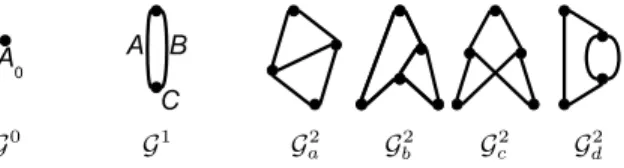
Definition 2.1 ([17]). A level-k generator (see Fig. 2) is a biconnected strict level-k network. Vertices of outdegree 0 and arcs of a level-k generator are called its sides, they are empty if no subtree is hanging from them. We call Sk the set of generators of level at most k, and Sk∗ the set of
level-k generators.
Phylogenetic networks have been defined above such that a level-k generator is a level-k phy-logenetic network (contrary to [17] we allow phylogenetic networks to contain hybrid vertices of outdegree 0). In particular, level-k generators and level-k networks are not allowed to contain vertices whose indegree and outdegree both equal 1.
Fig. 1. A level-2 network N with root ρ and leaf set {a, b, c, d, e, f, g, h, i, j, k}. All unlabeled vertices are split vertices. The gray area is a biconnected component with two hybrid vertices, namely r3
and r4. The arc from r2 to its child is a cut-arc. All arcs are directed downward but orientation is
not displayed for the sake of readability, as in the next figures.
G0 G1 G2 a G 2 b G 2 c G 2 d
Fig. 2. Level-0 generator G0, level-1 generator G1, and level-2 generators: Ga2, Gb2, Gc2 and Gd2.
2.2 Construction Rules
The level-0, respectively level-1, generator is called G0, respectively G1). In [17], the level-2 genera-tors are found by a case analysis which can also be applied to compute the 65 level-3 generagenera-tors [22]. Here we provide rules to compute all level-(k + 1) generators from level-k generators.
Definition 2.2. Let N be is a level-k generator. We define the following partial order N on its
sides: for two sides X and Y of N , Y N X if the source of arc Y (or Y itself, if Y is a vertex)
can be reached from the target of arc X (or X itself, if X is a vertex).
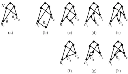
The network R1(N, X, Y ) is obtained by choosing two sides X and Y of N , such that if X = Y then X is not a hybrid vertex, and hanging a new hybrid vertex under X and Y (see Fig. 3).
The network R2(N, X, Y ) is obtained by choosing a side X of N and an arc Y 6 N X of N ,
and putting an arc from X to Y , which creates a new hybrid vertex “inside” arc Y .
Note that sides X and Y have a symmetric role for rule R1 but not for rule R2. When we build R1(N, X, Y ) from N , we say that we apply rule R1 on X and Y (and the same for R2). Note also that in the definition of R1(N, X, X), we only allow X to be an arc, or, in the particular case of N = G0, to be its only node.
Proposition 2.1. Let N be a level-k generator and X and Y two sides of N such that N1 =
R1(N, X, Y ), resp. N2 = R2(N, X, Y ), is well-defined. Then N1, resp. N2, is a level-(k + 1)
gener-ator.
Proof. We prove in Appendix A that in all cases, the rules provide a level-(k + 1) generator. ut
We have seen in Proposition2.1that we can build level-(k+1) generators from level-k generators, it remains to be proved that any level-(k + 1) generator can be obtained in this way.
Proposition 2.2. For any level-(k + 1) generator N , there exists a level-k generator N0, and some sides X and Y of N0 such that N = R1(N0, X, Y ) or N = R2(N0, X, Y ).
(a) (b) (c) (d) (e)
(f) (g) (h)
Fig. 3. Results of applying rules R1 and R2 on a level-2 generator N (a) depending on the type of side (arc or hybrid vertex) where it is applied: R1(N, h1, h2) (b), R1(N, e1, h2) (c), R1(N, e1, e1)
(d), R1(N, e1, e2) (e), R2(N, h2, e1) (f), R2(N, e1, e1) (g), R2(N, e2, e1) (h). In each case, a new
hybrid node, h3 is created.
Proof. The proof works by “reversing the rules” and finding an appropriate target vertex for the
reversed rule. It is detailed in Appendix B. ut
2.3 Bounding the Number of Generators
The rules we have defined can be used to obtain lower and upper bounds on the number of level-k generators.
Proposition 2.3. For k ≥ 1, a level-k generator has at most 3k − 1 vertices and 4k − 2 arcs.
Proof. The unique level-1 generator has two vertices and two arcs. By Proposition2.2, each level-k generator is obtained by applying rule R1 or R2 to a level-(k − 1) generator, hence by k applications of rules R1 or R2. We then notice that each application of rule R1 or R2 just adds at most three vertices and four arcs. The bounds are reached when R2 is repeatedly applied on two different arcs
as in Fig. 3(e). ut
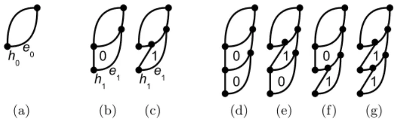
Proposition 2.4. The number gk of level-k generators is at least 2k−1.
Proof. The property is true for k = 0, so we fix k ≥ 1. We define an injection Gk between the
set of integers [0..2k−1− 1] and a set of level-k generators. The generator Gk(a) is build from the binary representation of a using only rule R1. The construction process is illustrated in Fig.4. Let a = Pk−2
i=0 ai2i ∈ [0..2k−1− 1] such that ai ∈ {0, 1}. We start with the level-1 generator G1, then
for i from 0 to k − 2:
(a) (b) (c) (d) (e) (f) (g)
Fig. 4. Construction of 2k−1 non-isomorphic level-k generators : we start from generator G1 (a) and apply R1(G1, e0, h0) to get G2(0) (b), G2(1) = R1(G1, e0, e0) (c), G3(0) = R1(G2(0), e1, h1)
(d), G3(1) = R1(G2(1), e1, h1) (e), G3(2) = R1(G2(0), e1, e1) (f), G3(3) = R1(G2(1), e1, e1) (g).
– let ei be the edge from the highest parent of hi (a simple proof by induction shows that there
always exists one parent of hi under the other).
– change G into R1(G, ei, hi) if ai=1, into R1(G, ei, ei) if ai= 0.
This way, we get for Gk(a) a digraph whose structure is a chain of cycles which encodes the binary
representation of a. Proposition2.1ensures that Gk(a) is a level-k generator. Thus, for each k, we
can build a set {Gk(a), a ∈ [0..2k−1− 1]} of 2k−1 level-k generators. These generators are obviously
non isomorphic, since they are each composed by a specific chain of two kinds of cycles. ut
Proposition 2.5. The number gk of level-k generators is lower than k!250k.
Proof. The previous proposition ensures that the number of arcs of a level-k generator is less than 4k, and its number of hybrid vertices is k, so its number of sides is less than 5k. When applying the kth rule R1 or R2, we choose a pair of sides, that is hybrid vertices or arcs, so there are less than (5k)2 possibilities. Thus gk+1 ≤ 2(5k)2gk< 50k2gk, so finally gk< k!250k. ut
Note that although these bounds are not tight, they give useful information on level-k generators. The lower bound shows that there is an exponential number of level-k generators, which implies, by the decomposition Theorem of Section 3, a great complexity inside the blobs of a network of high level. The upper bound for gk+1 from gk and the fact that g3 = 65 [22] shows that it seems
realistic to generate automatically level-4 and 5 generators at least.
2.4 The Generator Construction Algorithm
We now study how to use rules R1 and R2 in practice to build level-(k + 1) generators knowing the set of level-k generators. Note that different sequences of rules may produce isomorphic level-k generators. Hence, isomorphic level-k generators have to be removed in the process.
Theorem 2.1. There exists a polynomial algorithm which takes as input the set Sk∗ of all level-k generators and outputs the set of all level-(k + 1) generators.
Proof. The algorithm, BuildGenerators, detailed below, works by simply trying to apply rules R1 and R2 on any generator in Sk∗, then removing the isomorphic ones. To prove the polynomial complexity, the main point is the fact that the isomorphism test which is Graph Isomorphism-complete on general digraphs [35], can be done, in our case, in polynomial time [25,27] in the size
of the graph which is polynomial in |Sk∗| by propositions 2.3 and 2.4. The proof is also detailed in
Appendix D. ut
Algorithm 1: BuildGenerators builds the set S of level-(k + 1) generators from the set Sk∗ of level-k generators in polynomial time.
BuildGenerators(Sk∗: set of level-k generators)
S ← ∅
forall level-k generators g in Sk∗do
forall pairs (X, Y ) of sides of g do
if rule R1 can be applied on sides X and Y then g0← R1(g, X, Y )
forall level-(k + 1) generators h in S do
if g0 is not isomorphic to h then S ← S ∪ {g0} if rule R2 can be applied on sides X and Y then
g0← R2(g, X, Y )
forall level-(k + 1) generators h in S do
if g0 is not isomorphic to h then S ← S ∪ {g0} return S
Though graph isomorphism is decidable in polynomial time for graphs of bounded maximum degree, there exists no implementation of this algorithm, which seems difficult to use in prac-tice [23]. Instead, to actually build all level-4 generators from the 65 level-3 generators, we used an exponential time backtracking algorithm which tests isomorphism by trying to identify corre-sponding vertices by going through both input graphs at the same time. Among the 8501 level-4 generators built by applying rule R1 or R2, a total of 1993 are non-isomorphic. The list of these generators, the program to build them, its source and implementation notes are available at http://www.lirmm.fr/~gambette/ProgGenerators.php. Note that the sequence 1,4,65,1993 is not present in the On-Line Encyclopedia of Integer Sequences [31].
3 Generating Level-k Phylogenetic Networks
The concept of generator was introduced in [17] to build restrictions of level-k phylogenetic net-works, called simple, which contain no cut-arc except the trivial ones leading to leaves. We give an explicit composition theorem which shows how generators can be used to build any level-k network, and exhibits the link with the blobbed-tree structure of phylogenetic networks.
Definition 3.1. Given a set Sk of generators of level at most k, and a phylogenetic network N ,
we define the following rules, illustrated in Fig. 5:
– M ergeRootk(G0, G1) is obtained by hanging generators G0 and G1 ∈ Sk under a root.
– Attachk(v, G, N ) is the network obtained by adding an arc from hybrid vertex v ∈ N of outdegree
0 to a copy of a generator G ∈ Sk.
– Attachk(a, G, N ) is the network obtained by subdividing arc a (i.e. adding a vertex of indegree
(a) (b) (c) (d)
Fig. 5. Rules for building a level-k network from generators of level at most k: a phylogenetic network N (a); the network obtained by applying M ergeRootk(G0, G1) (b), Attachk(v, G0, N ) (c),
and Attachk(a, G0, N ) (d).
Note that rule M ergeRootk can be used only once, and that it is used for level-k networks that
are disconnected when removing their root.
Theorem 3.1. N is a level-k network iff there exists a sequence of r ∈ N locations (arcs or hybrid vertices) (`j)j∈[1,r] and a sequence of generators (Gj)j∈[0,r] in Sk, such that:
N = Attachk(`r, Gr, Attachk(. . . Attachk(`2, G2, Attachk(`1, G1, G0)) . . .)),
or N = Attachk(`r, Gr, Attachk(. . . Attachk(`2, G2, M ergeRootk(G1, G0)) . . .)).
Proof. The proof works by induction and is detailed in Appendix C. ut
Theorem 3.1 characterizes level-k networks by a sequence of rules on a finite set of generators. In this form, the characterization does not yield canonicity: two different sequences of rule appli-cations may lead to the same phylogenetic network (typically, by just changing the order in which rules are applied).
However, this characterization is deeply based on a canonical tree decomposition of level-k networks which by lack of space cannot be detailed here, but is illustrated in Figure 6. It enters
Fig. 6. A level-2 phylogenetic network and its canonical decomposition tree: each node of the tree contains a generator of level ≤ k; each arc of the tree is linked to a side of the generator at the source node, and labeled by an integer showing in which order it is attached to the side, if the side is an arc.
counting or efficient exhaustive generation of level-k phylogenetic networks, which would extend currently known results on the number of unicyclic networks and galled trees [32].
4 Level-k Networks and the Coalescent Model with Recombination
In [2], Arenas et al conducted a simulation study to generate a number of realistic phylogenetic networks, according to the coalescent model with recombination, and measure the proportion of these networks contained in different subclasses of phylogenetic networks, among which trees and galled trees, i.e. level-0 and level-1 phylogenetic networks. We extend their study by computing the level of a sample of phylogenetic networks generated by the program Recodon [1]. The Java implementation of a simple biconnected component decomposition algorithm to compute the level is also available at http://www.lirmm.fr/~gambette/ProgGenerators.php.
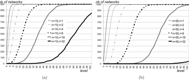
For small levels, the results we obtained are shown in Table1, and an insight on upper levels is given in Fig.7.
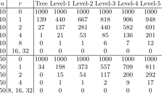
n r Tree Level-1 Level-2 Level-3 Level-4 Level-5 10 0 1000 1000 1000 1000 1000 1000 10 1 139 440 667 818 906 948 10 2 27 137 281 440 582 691 10 4 1 21 53 85 136 201 10 8 0 1 1 6 7 12 10 16, 32 0 0 0 0 0 0 50 0 1000 1000 1000 1000 1000 1000 50 1 34 198 373 557 709 811 50 2 0 15 54 117 200 292 50 4 0 1 1 2 9 17 50 8, 16, 32 0 0 0 0 0 0
Table 1. Number of simulated networks falling in each class as a function of the recombination rate r = 0, 1, 2, 4, 8, 16, and 32 for sample size n = 10 or n = 50.
We observe that phylogenetic networks with a small level, like restricted phylogenetic networks formerly studied (regular, tree-sibling and tree-child, see [2]), cover a small portion of the networks corresponding to the coalescent model with high recombination rates. Still, the proportion of level-2 phylogenetic networks for 10 leaves is greater than the proportion of tree-child networks, but to get similar proportions on 50 leaves we have to consider level-3 networks.
In fact, our results show that level-k phylogenetic networks do not have a blobbed-tree structure in the context of the coalescent model. Instead, most of the simulated networks have all their hybrid vertices inside one same blob. This phenomenon even appears with a small recombination rate, as shown in Fig.8. Thus, for this context, new structures and algorithmic techniques have to be found.
The coalescent model is not suitable to describe all cases of reticulate evolution. For example, a simple model of horizontal gene transfer based on inserting transfer events according to a Poisson distribution, respecting time constraints was given in [8]. The use of phylogenetic networks of bounded level may be more appropriate for this model, or others [28].
(a) (b)
Fig. 7. Level-k phylogenetic networks and the coalescent model with recombination: for recom-bination rates r =1, 2, 4, 8, 16, 32, the number of phylogenetic networks of level-k is shown, for simulations on 10 leaves (a) and on 50 leaves (b).
Fig. 8. Number of reticulations and level of the simulated networks for n = 10 and r = 1. The size of the dot at position (x, y) reflects the number of strict level-x networks with y hybrid vertices.
Acknowledgments
We thank the French ANR projects ANR-06-BLAN-0148-01 (GRAAL) and ANR-08-EMER-011-01 (PhylARIANE) for support. We thank Steven Kelk, Leo van Iersel, Katharina Huber and Matthias Mnich for their comments on earlier versions of this paper. We thank Michael Rao for his help on the isomorphism test for level-k generators, and Gabriel Valiente and Miguel Arenas for sharing their simulated data on the coalescent model.
References
1. Miguel Arenas and David Posada. Recodon: Coalescent Simulation of Coding DNA Sequences with Recombination, Migration and Demography. BMC Bioinformatics 8, 458 (2007).
2. Miguel Arenas, Gabriel Valiente and David Posada. Characterization of Reticulate Networks based on the Coa-lescent with Recombination. Molecular Biology and Evolution 25(12), 2517–2520 (2008).
3. Jaroslaw Byrka, Pawel Gawrychowski, Katharina T. Huber and Steven Kelk. Worst-case Optimal Approximation Algorithms for Maximizing Triplet Consistency within Phylogenetic Networks. Journal of Discrete Algorithms, to appear (2009).
4. Ho-Leung Chan, Jesper Jansson, Tak-Wah Lam and Siu-Ming Yiu.. Reconstructing an Ultrametric Galled Phy-logenetic Network from a Distance Matrix. Journal of Bioinformatics and Computational Biology 4(4), 807–832 (2006).
5. Charles Choy, Jesper Jansson, Kunihiko Sadakane, and Wing-Kin Sung. Computing the Maximum Agreement of Phylogenetic Networks. Theoretical Computer Science 335(1), 93–107 (2005).
6. Gabriel Cardona, Francesc Rossell´o and Gabriel Valiente. Comparison of Tree-Child phylogenetic networks. IEEE/ACM Transactions in Computational Biology and Bioinformatics, to appear (2009).
7. Joost Engelfriet and Vincent van Oostrom. Logical Description of Contex-Free Graph Languages. J. Comput. Syst. Sci. 55(3), 489–503 (1997).
8. Nicolas Galtier. A Model of Horizontal Gene Transfer and the Bacterial Phylogeny Problem. Systematic Biology 56, 633–642, 2007.
9. Philippe Gambette. Who is Who in Phylogenetic Networks: Articles, Authors and Programs.http://www.lirmm. fr/~gambette/PhylogeneticNetworks.
10. Emeric Gioan and Christophe Paul. Split Decomposition and Graph-Labelled Trees: Characterizations and Fully-Dynamic Algorithms for Totally Decomposable Graphs. Submitted (2009).
11. Dan Gusfield and Vikas Bansal. A Fundamental Decomposition Theory for Phylogenetic Networks and Incom-patible Characters. In RECOMB 2005. LNCS, vol. 3500, pp. 217–232. Springer (2005).
12. Dan Gusfield, Satish Eddhu, and Charles Langley. Efficient Reconstruction of Phylogenetic Networks with Constrained Recombination. In Proceedings of the 2003 IEEE Computational Systems Bioinformatics Conference (CSB2003), pp. 363–374 (2003).
13. Verne Grant. Plant Speciation, pp. 300–320, 383–386. Columbia University Press (1971).
14. Mike Hallett and Jens Lagergren. Efficient Algorithms for Lateral Gene Transfers Problems. In Proceedings of the fifth Annual International Conference on Research in Computational Molecular Biology (RECOMB’01), pp. 141–148 (2001).
15. Richard R. Hudson. Properties of the Neutral Allele Model with Intragenic Recombination. Theoretical Population Biology 23, 183–201 (1983).
16. Daniel H. Huson. Split Networks and Reticulate Networks. In Olivier Gascuel and Mike Steel (eds.) Reconstructing Evolution, pp. 247–276. Oxford University Press (2007).
17. Leo van Iersel, Judith Keijsper, Steven Kelk, Leen Stougie, Ferry Hagen, and Teun Boekhout. Constructing Level-2 Phylogenetic Networks from Triplets. In RECOMB 2008. LNCS vol. 4955, pp. 450–462. Springer (2008). 18. Leo van Iersel and Steven Kelk. Constructing the Simplest Possible Phylogenetic Network from Triplets. In
ISAAC 2008. LNCS vol. 5369, pp. 472–483. Springer (2008).
19. Leo van Iersel, Steven Kelk and Matthias Mnich. Uniqueness, Intractability and Exact Algorithms: Reflections on Level-k Phylogenetic Network. To appear in Journal of Bioinformatics and Computational Biology (2009). 20. Jesper Jansson and Wing-Kin Sung. Inferring a Level-1 Phylogenetic Network from a Dense Set of Rooted
Triplets. Theoretical Computer Science 363(1), 60–68 (2006).
21. Iyad A. Kanj, Luay Nakhleh, Cuong Than and Ge Xia. Seeing the Trees and Their Branches in the Network is Hard. Theoretical Computer Science 401, 153–164 (2008).
22. Steven Kelk. http://homepages.cwi.nl/~kelk/lev3gen/.
23. Volker Kaibel and Alexander Schwartz. On the Complexity of Polytope Isomorphism Problems. Graphs and Combinatorics 19(2), 215-230 (2003).
24. C. Randal Linder and Loren H. Rieseberg. Reconstructing Patterns of Reticulate Evolution in Plants. American Journal of Botany 91(10), 1700–1708 (2004).
25. Eugene M. Luks. Isomorphism of Graphs of Bounded Valence Can be Tested in Polynomial Time. Journal of Computer and System Sciences 25(1), 42–65 (1982).
26. Dave MacLeod, Robert L. Charlebois, W. Ford Doolittle, and Eric Bapteste. Deduction of Probable Events of Lateral Gene Transfer through Comparison of Phylogenetic Trees by Recursive Consolidation and Rearrangement. BMC Evolutionary Biology 5, 27 (2005).
27. Gary L. Miller. Graph Isomorphism, General Remarks. In Proceedings of the Ninth Annual ACM Symposium on Theory of Computing (STOC’77), pp. 143–150 (1977).
28. Monique M. Morin and Bernard M. E. Moret. NetGen: Generating Phylogenetic Networks with Diploid Hybrids. Bioinformatics 22(15), 1921–1923 (2006).
29. Bin Ma, Lusheng Wang and Ming Li. Fixed Topology Alignment with Recombination. In CPM 1998, LNCS, vol. 1448, pp. 174–188. Springer (1998).
30. Luay Nakhleh and Tandy Warnow and C. Randal Linder and Katherine St. John. Reconstructing Reticulate Evolution in Species - Theory and Practice. Journal of Computational Biology 12(6), 796–811 (2005).
31. Neil J.A. Sloane. The On-Line Encyclopedia of Integer Sequences. Published electronically at http://www. research.att.com/~njas/sequences/.
32. Charles Semple and Mike Steel. Unicyclic Networks: Compatibility and Enumeration. IEEE/ACM Transactions in Computational Biology and Bioinformatics 3, 398–401 (2004).
33. Thu-Hien To and Michel Habib. Level-k Phylogenetic Network can be Constructed from a Dense Triplet Set in Polynomial Time. In CPM 2009, to appear (2009).
34. Lusheng Wang, Kaizhong Zhang, and Louxin Zhang. Perfect phylogenetic networks with recombination. In Proceedings of the 16th ACM Symposium on Applied Computing (SAC’01), pp. 46–50 (2001).
35. V. N. Zemlyachenko, Nickolay M. Korneenko, and Regina I. Tyshkevich. Graph Isomorphism Problem. Journal of Mathematical Sciences 29(4), 1426–1481 (1985).
Appendix A
We recall Proposition2.1and prove it.
Proposition 4.1. Let N be a level-k generator and X and Y two sides of N such that N1 =
R1(N, X, Y ), resp. N2 = R2(N, X, Y ), is well-defined. Then N1, resp. N2, is a level-(k + 1)
gener-ator.
Proof. Since N1 and N2 are well-defined, sides X and Y meet the requirements imposed in
Def-inition 2.2 for R1 and R2. These definitions ensure that the acyclicity of the graph is preserved. Thus, we just have to show that for any type of sides (arc or hybrid vertex) X and Y (as detailed in Fig. 3), applying rule R1 or R2 always adds split vertices and exactly one hybrid vertex, with outdegree ≤ 1.
We first check what happens when applying rule R1 to get R1(N, X, Y ): – if N = G0, then applying R1 gives the level-1 generator G1.
– if X and Y are distinct hybrid vertices, they have outdegree 0 as they are sides of N , so applying R1 will just give them outdegree 1, and create a new hybrid vertex of outdegree 0 (Fig. 3(b)). – if X is a hybrid vertex, and Y is an arc, then applying R1 gives X outdegree 1, adds a new hybrid vertex of outdegree 0 and creates a new split vertex “inside” Y (whose parent is the upper extremity of Y , and whose children are the lower extremity of Y and the new hybrid vertices created), as shown in Fig. 3(c). By symmetry we also get a valid generator if X is an arc and Y is a hybrid vertex.
– if X and Y are both arcs (possibly the same as in Fig.3(d)) then applying R1 creates two split vertices, one inside X and the other inside Y (Fig. 3(e)).
In all cases R1(N, X, Y ) is obtained from N by adding a hybrid vertex and possibly some split ver-tices. Thus R1(N, X, Y ) meets the definition of a strict level-(k + 1) network. As the transformation preserves biconnectivity, then R1(N, X, Y ) is a level-(k + 1) generator.
We now check what happens when applying rule R2 to get R2(N, X, Y ):
– if X is a hybrid vertex, and Y is an arc, then applying R2 gives X outdegree 1, and creates a new hybrid vertex of outdegree 1 “inside” Y (whose parents are X and the upper extremity of Y , and whose child is the lower extremity of Y ), as shown in Fig. 3(f).
– if X and Y are both arcs (possibly the same, see Fig. 3(g)) then applying R1 creates a split vertex inside X and a hybrid vertex of outdegree 0 inside Y (Fig. 3(h)).
In all cases R2(N, X, Y ) is obtained from N by adding a hybrid vertex and possibly some split vertices so, similarly as above, R2(N, X, Y ) is a level-(k + 1) generator. ut
Appendix B
The proof of Proposition2.2directly follows from Lemma 4.1detailed below. But we first need to define the removal of a hybrid vertex by reversing rules R1 and R2.
Definition 4.1. Let N be a level-(k + 1) phylogenetic network, and v a vertex of N , that is not a child of the root, except for the case where N = G1. We define the R1R2-removal of v, which provides a level-k network N0, in the following way. The vertex v is first removed from the graph with all its adjacent arcs; then, in several cases, arcs are added to the network to maintain connectivity.
(a) the parents of v are distinct hybrid vertices X and Y , then by deleting v, vertices X and Y get outdegree 0, and no other vertex is changed, as shown in Fig. 9(a). If we call N0 the network obtained after deletion then we note N = R1(N0, X, Y ),
(b) a parent of v, say Y , is a hybrid vertex and the other, X, is a split vertex, then, as shown in Fig. 9(b), by deleting v, X, and joining the parent of X to the second child of X (other than v) thanks to arc eX, we get a network N0 such that N = R1(N0, Y, eX),
(c) the parents of v are split vertices X and Y such that X is neither a child nor the parent of Y , cf. Fig. 9(c). Then, by deleting v, X, Y , and joining the parent of X to the second child of X (other than v) thanks to an arc eX, and the parent of Y to the second child of Y (other than v)
thanks to an arc eY, we get a network N0 such that N = R1(N0, eX, eY).
(d) the parents of v are split vertices X and Y where X is the parent of Y , cf. Fig. 9(d). Then, by deleting v, X, Y , and joining the parent of X to the second child of Y (other than v) thanks to an arc eXY, we get a network N0 such that N = R1(N0, eXY, eXY).
(e) v is the only child of the root, then N has to be G1, as shown in Fig.9(e), we remove v and its two incoming arcs to get the level-0 generator N0 = G0 with one vertex A0 and N = R1(N0, A0, A0).
If v has outdegree 1, then three cases arise:
(f ) at least one parent of v, say Y , is a hybrid vertex. Then by deleting v, and joining X to the child of v thanks to arc eX, vertex Y gets outdegree 0 and the degree of no other vertex is changed,
as shown in Fig. 9(f ), we get a network N0 such that N = R2(N0, Y, eX),
(g) both parents of v are different split vertices X and Y , then, as shown in Fig. 9(g), by deleting v, Y , and joining the parent of Y to the second child of Y (other than v) thanks to arc eY, and
joining X to the child of v thanks to arc eX, we get a network N0 such that N = R2(N0, eY, eX).
(h) v only has one parent which is the split vertex X, then, as shown in Fig. 9(h), by deleting v, X, and joining the parent of X to the child of v thanks to arc eX, we get a network N0 such
that N = R2(N0, eX, eX).
(a) (b) (c) (d) (e) (f) (g) (h)
Fig. 9. Different possible cases to “reverse” rules R1 and R2, depending on whether the rule has created an outdegree 0 hybrid vertex (a-e) which corresponds to rule R1 or an outdegree 1 hybrid vertex (f-h) which corresponds to rule R2: gray arcs and vertices are to be deleted to reverse the rule.
Note that, in each case, the nodes of N0 meet the degree requirements stated in the definition of a phylogenetic network. Reusing the names R1 and R2 above is an abuse of notation as we have no guarantee yet, when we write N = Ri(N0, X, Y ) in this definition of reversed rules, that N0 is a generator, nor that X and Y are sides. However, we will only use them in such proper cases.
Lemma 4.1. Let N be a level-(k + 1) generator. There exists a vertex v of N such that the R1R2-removal of v from N gives a level-k generator.
Proof. We prove it by induction. Base case:
Call A0 the only vertex of G0, A and B the two arcs of G1, and C its hybrid vertex. Then we
can check the base cases for k ≤ 1 (see Fig. 2) as G1= R1(G0, A0, A0) (vertex C is R1R2-removed,
we are in case (e)), and for k = 1 we remove hybrid vertices which are not children of the root: G2
a= R1(G1, B, C) (b), Gb2 = R1(G1, B, B) (d), Gc2 = R1(G1, A, B) (c) and Gd2= R2(G1, B, B) (h).
Inductive step:
We now fix k ≥ 2. We suppose that the expected property is true for any level-j generator, with j < k and prove it for level k. So consider a level-(k + 1) generator N . It contains at least three hybrid vertices, so at least one of the three, say v, is not a child of the root. Then, we R1R2-remove it, and obtain a level-k network N0.
We now have to prove that either N0 is a level-k generator, or we can directly choose another hybrid vertex v00 whose R1R2-removal gives a level-k generator.
If N0 is biconnected, then by definition of a generator, it is a level-k generator.
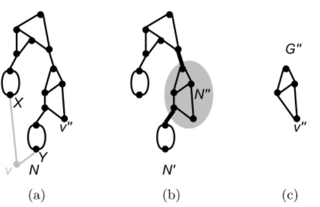
Assume N0 is not biconnected as illustrated in Fig. 10. Let N00 be a biconnected component of N0 which does not contain the root. Note that by definition 4.1, the R1R2-removal of v from N did not create any leaf in N0, therefore N00 is a non-trivial biconnected component, so it hosts at least one hybrid vertex. Either N00 is a level-j generator with 0 < j < k, then we call it G00.
Otherwise, it is not even a level-k phylogenetic network because of the degree requirements. We claim that in this case N00 contains exactly one vertex having both indegree and outdegree 1. Indeed, N00 is only connected by cut-arcs to the rest of N0. As N is biconnected, the presence of biconnected components in N0 results from the R1R2-removal of v. Since v has indegree 2, N0 contains at most two cut-arcs incident to vertices of N00, as shown in Fig. 10(b). One of those cut-arcs leads to the root of N00, as N00 does not contain the root of N0, so there is at most one cut-arc hanging from N00 in N0. This is the only problematic point which impedes N00 from being a generator, as it reflects the presence of an indegree and outdegree 1 vertex when considering N00 by itself. In this case, we consider the level-j generator G00 obtained by deleting this vertex, and connecting its parent to its child in N00.
(a) (b) (c)
Fig. 10. If removing v disconnects the graph, then we find another vertex v00 which can be R1R2-removed to get a level-(k − 1) generator.
In both cases, we apply the induction hypothesis on this level-j generator G00: as j > 0, it contains a hybrid vertex v00, that can be R1R2-removed. Even if the R1R2-removal of v00 from G00 gives a valid level-(j − 1) generator, where biconnectivity is preserved, it remains to prove that the R1R2-removal of v00 from N gives a valid level-(k − 1) generator. Fig. 10 shows that this is not always straightforward: in the depicted case, one parent of v00in G00 is a split vertex and the other one is a hybrid vertex, which corresponds to case (b) for the R1R2-removal of v00, whereas in N , both parents of v00 are split vertices, which corresponds to case (c). Hence we have to show which case of the R1R2-removal applies in N depending on the one applying in the context of G00.
Let X00 and Y00 be the parents of v00 in G00 (we name X00 and Y00 similarly to X and Y in the definition of R1R2-removal). We recall that each case is illustrated in Fig.9.
We first consider case (a). If v00 also has outdegree 0 in N then:
– if both parents of v00 in N are hybrid vertices, then R1R2-remove v00 from N according to case (a).
– if exactly one of the parents of v00 in N is not a hybrid vertex, then R1R2-remove v00 from N according to case (b).
– if no parent of v00 in N is a hybrid vertex, then R1R2-remove v00 from N according to case (c). Otherwise, v00 has outdegree 1 in N then R1R2-remove v00 according to case (f ). Note that it is impossible that neither X00 nor Y00 is the parent of v00 in N : as there is already an arc under v00 in N , there can only be one other arc (leading to v, or cut-arc in N0) hanging from N00 (thus creating a split vertex under one of v00’s parent and over v00) in N .
We now consider case (b). If v00 also has outdegree 0 in N then the same applies as in case (a). Otherwise, v00 has outdegree 1 in N :
– if one of the parents of v00 in N is a hybrid vertex, then R1R2-remove v00in N according to case (f ).
– otherwise R1R2-remove v00 from N according to case (g). We now consider case (c). If v00 also has outdegree 0 in N then:
– if exactly one of the parents of v00 in N is a hybrid vertex, then R1R2-remove v00 from N according to case (b).
– otherwise R1R2-remove v00 from N according to case (c).
Otherwise, v00 has outdegree 1 in N , the same applies as in case (b).
We now consider case (d). If v00 also has outdegree 0 in N then, if X00 and Y00 are still the parents of v00 in N then R1R2-remove v00 from N according to case (d), otherwise:
– if exactly one of the parents of v00 in N is a hybrid vertex, then R1R2-remove v00 from N according to case (b).
– otherwise R1R2-remove v00 from N according to case (c).
Otherwise, v00 has outdegree 1 in N , the same applies as in case (b).
We now consider case (e). If v00 also has outdegree 0 in N then, the case where v00 still has only one parent in N cannot happen (otherwise N would not be biconnected), so:
– if exactly one of the parents of v00 in N is a hybrid vertex, then R1R2-remove v00 from N according to case (b).
Otherwise, v00 has outdegree 1 in N . If v00 still has only one parent in N then R1R2-remove v00 according to case h, otherwise the same applies as in case (b).
We now consider cases (f ) and (g):
– if one of the parents of v00 in N is a hybrid vertex, then R1R2-remove v00in N according to case (f ).
– otherwise R1R2-remove v00 from N according to case (g).
We finally consider case (h): if v00still has only one parent in N then R1R2-remove v00according to case (h), otherwise the same applies as in case (f ).
We can also check in all these cases that R1R2-removing v00 from N maintained the biconnec-tivity ensured when R1R2-removing v00 from G00.
In any case, we have found a hybrid vertex which can be removed to get a level-k generator,
therefore the proposition is true. ut
Appendix C
We recall Theorem3.1and prove it.
Theorem 4.1. N is a level-k network iff there exists a sequence of r ∈ N locations (arcs or hybrid vertices) (`j)j∈[1,r] and a sequence of generators (Gj)j∈[0,r] in Sk, such that:
N = Attachk(`r, Gr, Attachk(. . . Attachk(`2, G2, Attachk(`1, G1, G0)) . . .)),
or N = Attachk(`r, Gr, Attachk(. . . Attachk(`2, G2, M ergeRootk(G1, G0)) . . .)).
Proof. ⇐: This implication is trivially proved by induction, as any sequence of the above rules repeatedly attaches one or two new biconnected components (each containing at most k hybrid vertices) by cut-arcs to the structure already built.
⇒: We prove by induction on the number p of vertices of a level-k phylogenetic network N , that for any k ∈ N, N can be obtained by repeated applications of the Attach rule after a possible initial application of the M ergeRoot rule.
Base case: if p = 1 then the only possible network is G0, which corresponds to not applying any rule (take r = 0 in the theorem) to the level-0 generator G0.
Inductive step: now suppose that all networks with strictly less than p vertices verify the de-sired property, let N be a network with p vertices.
A. If N contains a leaf l, then:
i) either l has at least one grand-parent, say u, then:
• either the parent of u is a split vertex, then delete l, its parent, and connect the grand-parent u to the sibling v of u. The obtained network N0 has less than p vertices, so the induction hypothesis applies, and the observation that
N = Attachk((u, v), G0, N0),
• either the parent of l is a hybrid vertex h, then delete l, and (h, l). The obtained net-work N0 has less than p vertices, so the induction hypothesis applies, and since N = Attachk(h, G0, N0), the desired property is true for N .
ii) Otherwise, l has no grand-parent, that is its parent is the root. Then the network N0 obtained by considering the sibling u of l and the subnetwork rooted at u has less than p vertices, so we can apply the induction hypothesis, from which we have:
• either
N0= Attachk(`r, Gr, Attachk(. . . (1)
Attachk(`2, G2, Attachk(`1, G1, G0)) . . .)),
then
N = Attachk(`r, Gr, Attachk(. . .
Attachk(`2, G2, Attachk(`1, G1, M ergeRootk(G0, G0))) . . .))
• or
N0 = Attachk(`r, Gr, Attachk(. . . (2)
Attachk(`2, G2, M ergeRootk(G1, G0)) . . .)).
then
N = Attachk(`r, Gr, Attachk(. . .
Attachk(`2, G2, Attachk(`0, G1, M ergeRoot(G0, G0))) . . .)),
where `0 is the arc from the root to G0 in M ergeRoot(G0, G0).
B. If N contains no leaf, it only contains a root, split and hybrid vertices.
i) either N is biconnected, then it is a generator, and it has k hybrid vertices or less (as N is level-k), so the expected property is true.
ii) otherwise, N is not biconnected, and N has a hybrid vertex of outdegree 0. Consider its bi-connected component tree. Consider a leaf of this tree, that is one of the “lowest” bibi-connected components. Let C be this biconnected component, i.e. C is a level-k generator. We treat C exactly like leaf l in equations (1) and (2) above, by replacing G0 by C in the decomposition formulas.
u t
Appendix D
We recall Theorem2.1and prove it.
Theorem 4.2. There exists a polynomial algorithm which takes as input the set Sk∗ of all level-k generators and outputs the set Sk+1∗ of all level-(k + 1) generators.
Proof. The algorithm, BuildGenerators, is described in Algorithm 1.
By the proof of Proposition 2.5, rules R1 and R2 are applied at most 50k2|S∗
k| times in the
algorithm. Proposition2.4ensures that |Sk∗| ≥ 2k−1, so k = o(|S∗
k|), and by Proposition2.3the size
of a generator is also polynomial in |Sk∗|. Hence, the number of isomorphism tests is polynomial in |S∗
k|.
To prove that this algorithm is polynomial in the size of the input Sk∗, we prove that the isomorphism test can be done in polynomial time in k.
Digraph isomorphism is Graph Isomorphism-complete [35], which implies that no polynomial algorithm is currently known for this problem in the general case. However, here we restrict to instances where the digraphs have maximal degree 3 in particular, and isomorphism for graphs of bounded maximum degree can be determined in polynomial time [25]. We now show how to polynomially reduce the problem of isomorphism for digraphs of maximum degree 3 and maximum outdegree and indegree 2 to the problem of isomorphism for graphs of bounded degree.
For each digraph D whose vertices all have degree at most 3, outdegree and indegree at most 2, and possibly multiple arcs, we use the gadget introduced by Miller [27] to build a graph G(D) in the following way:
– all vertices of D are vertices of G(D),
– every arc (u, v) of D is transformed into a P4graph u − u0− v0− v, completed with a P2 attached
to u0 and a P3 to v0.
(a) (b)
Fig. 11. A digraph D (a) and the associated undirected graph G(D) (b) by a transformation introduced by Miller [27] which preserves isomorphism and bounded degree.
This construction, illustrated in Fig. 11, is done in a time that is polynomial to the size of the digraph and provides an undirected graph of maximum degree 3. It ensures that D1 is isomorphic