Conceptual engineering design and optimization methodologies using geometric programming

Conceptual Engineering Design and Optimization

Methodologies using Geometric Programming

by

Berk Öztürk

B.S., Massachusetts Institute of Technology, 2016

Submitted to the Department of Aeronautics and Astronautics

in partial fulfillment of the requirements for the degree of

Master of Science in Aeronautics and Astronautics

at the

MASSACHUSETTS INSTITUTE OF TECHNOLOGY

February 2018

© Massachusetts Institute of Technology 2018. All rights reserved.

Author . . . .

Department of Aeronautics and Astronautics

February 1st, 2018

Certified by. . . .

Mark Drela

Professor, Aeronautics and Astronautics

Thesis Supervisor

Accepted by . . . .

Hamsa Balakrishnan

Associate Professor, Aeronautics and Astronautics

Chair, Graduate Program Committee

Conceptual Engineering Design and Optimization

Methodologies using Geometric Programming

by

Berk Öztürk

Submitted to the Department of Aeronautics and Astronautics on February 1st, 2018, in partial fulfillment of the

requirements for the degree of

Master of Science in Aeronautics and Astronautics

Abstract

Geometric programs (GPs) and other forms of convex optimization have recently ex-perienced a resurgence due to the advent of polynomial-time solution algorithms and improvements in computing. Observing the need for fast and stable methods for mul-tidisciplinary design optimization (MDO), previous work has shown that geometric programming can be a powerful framework for MDO by leveraging the mathemati-cal guarantees and speed of convex optimization. However, there are barriers to the implementation of optimization in design. In this work, we formalize how the for-mulation of non-linear design problems as GPs facilitates design process. Using the principles of pressure and boundedness, we demonstrate the intuitive transformation of physics- and data-based engineering relations into GP-compatible constraints by systematically formulating an aircraft design model. We motivate the difference-of-convex GP extension called signomial programs (SPs) in order to extend the scope and fidelity of the model. We detail the features specific to GPkit, an object-oriented GP formulation framework, which facilitate the modern engineering design process. Using both performance and mission modeling paradigms, we demonstrate the ability to model and design increasingly complex systems in GP, and extract maximal engi-neering intuition using sensitivities and tradespace exploration methods. Though the methods are applied to an aircraft design problem, they are general to models with continuous, explicit constraints, and lower the barriers to implementing optimization in design.

Thesis Supervisor: Mark Drela

Acknowledgments

Firstly, I would like to thank Professor Warren Hoburg for giving me the opportunity to work on research that I believe has great potential. He introduced me to geomet-ric programming and welcomed me to the Hoburg Research Group (now the Convex Engineering Group). Under his mentorship, I learned that the most interesting de-signs are the ones we don’t expect, and that challenging current engineering design methods and norms is the most worthwhile objective of optimization. So thank you for the opportunity to do just that.

I am grateful for the many friends I have in the Aerospace Computational Design Lab (ACDL) who have lightened my work hours with their camaraderie. Of this group, the Convex folks reserve a special place. I am lucky to collaborate with such a talented and dedicated group of researchers, and I hope that we will continue to redefine conceptual engineering design.

This thesis would not have been possible without the amazing work Ned Burnell does as the lead developer of GPkit. He never ceases to amaze me with his creativity and energy. The many debates we have had about design philosophy have inspired this thesis, and I’m glad I’ve gotten the opportunity to extensively document many of the ideas that were discussed.

I thank my co-advisors Professor Mark Drela and Bob Haimes, who have taken on the burden of advising me in Woody’s absence. Thank you for your guidance and wisdom, and pushing me to finish this thesis.

I am indebted to cycling for keeping me fit and sane. Cycling has given me opportunities to escape, even as I miss winter training camp to conclude this thesis. MIT Cyclists have been an immutable source of joy in my life, and are near and dear to my heart. Thanks for enabling me.

I would like to thank my long-time friend Johannes Norheim for being a battle-scarred companion through 5 years of MIT. We have been challenged, and our paths have converged and diverged many times, but our friendship has not wavered. My partner Elise Newman has been a ray of sunshine in every weather, and I am looking

forward to our future adventures together.

My parents definitely deserve a mention because I wouldn’t exist without them. The longer I live, the more I understand that I am where I am because of the sacrifices they have made. Deniz, you have been my rock. It has been my privilege to be your brother and watch you grow up, and will be my privilege to help you through your struggles and celebrate your future successes. I am confident you will be more than I have been.

Contents

1 Introduction 13

1.1 Distinguishing between design and optimization . . . 14

1.2 Unifying design and optimization with GP . . . 16

2 Engineering inequalities and intuition, from equalities 19 2.1 Making feasibility sets and boundedness explicit . . . 19

2.2 Defining the design problem . . . 22

2.2.1 Objective functions . . . 22

2.2.2 Functional description: constraining the problem . . . 23

2.3 GP modeling from physics . . . 23

2.3.1 Free and fixed variables: weight and lift model . . . 24

2.3.2 Alternate objectives: more performance metrics . . . 26

2.3.3 More physics for boundedness: thrust and drag model . . . 27

2.4 Limits of GP and convexity, and SP modeling . . . 30

2.4.1 Signomial constraints: fuel volume model . . . 30

2.4.2 Arguments for the signomial equality . . . 32

2.4.3 Completing the model: wing structural model . . . 33

2.5 Results of SimPleAC . . . 34

3 Extensibility of GP 37 3.1 Modularization and improved fidelity: engine model . . . 37

3.1.1 Creating an engine submodel . . . 37

3.1.3 Converting all subsystems into submodels . . . 41

3.2 Mission design and performance modeling form . . . 42

3.2.1 Linking performance models: flight segments . . . 46

3.2.2 Characterizing the environment: atmospheric model . . . 47

3.2.3 Mission objectives . . . 48

3.3 Design exploration through mission design . . . 48

3.4 More modeling improvements before multimission design . . . 51

3.4.1 Environmental effects: engine lapse rate model . . . 52

3.4.2 Making use of sensitivities: engine BSFC model . . . 52

3.5 Multimission design . . . 53

3.5.1 Multimission objective functions . . . 54

3.5.2 Multimission optimization results . . . 55

3.5.3 Potential extensions of multimission design . . . 57

4 Conclusion 59 A Mathematical Framework 61 A.1 Geometric Programming . . . 61

A.2 Signomial Programming . . . 62

B Model Resources 65 B.1 Flight segment model variables . . . 65

List of Figures

1-1 The flow diagrams of two methods of optimization. . . 17 2-1 The 𝑥-𝑦 feasibility set of a simple monomial equality. . . 20 2-2 The 𝑥-𝑦 feasibility set of lower-bounding monomial, and upper-bounding

posynomial. . . 21 2-3 The 𝑥-𝑦 feasibility set of upper-bounding monomial, and upper-bounding

posynomial. . . 21 3-1 Engine MSL power versus weight fits for 𝐾 = 1, 2 posynomial terms

with underlying data. . . 40 3-2 Variable and constraint hierarchy of the SimPleAC model for a single

flight segment. . . 41 3-3 Variable and constraint hierarchy of the SimPleAC static+performance

model for two flight segments. . . 42 3-4 Variable hierarchy of thrust constraint 3.4. . . 46 3-5 The fuel and total weight contours with respect to range and payload. 49 3-6 Fraction of total fuel stored in fuselage with respect to range and payload. 50 3-7 Time cost and time cost index sensitivity contours. . . 50 3-8 BSFC

BSFC𝑚𝑖𝑛 versus

𝑃𝑠ℎ𝑎𝑓 𝑡

𝑃𝑠ℎ𝑎𝑓 𝑡,𝑎𝑙𝑡 data fit. . . 53

3-9 Multimission uni-directional graph, with 𝑁𝑠𝑒𝑔𝑚𝑒𝑛𝑡𝑠= 2and 𝑁𝑚𝑖𝑠𝑠𝑖𝑜𝑛𝑠 = 2. 54

A-1 A signomial inequality constraint and GP approximations about two different points. . . 64 A-2 The signomial equality constraint 𝐶𝐷 = 𝑓 (𝐶𝐿) and its approximation. 64

List of Tables

2.1 Variables introduced in the weight and lift model. . . 25

2.2 Variables introduced to define new performance metrics. . . 26

2.3 Unbounded variables in the weight and lift model. . . 27

2.4 Variables introduced in the thrust and drag model. . . 29

2.5 Unbounded variables in the GP-compatible formulation. . . 29

2.6 Variables introduced in the fuel model. . . 32

2.7 Variables introduced in the wing structural model. . . 34

2.8 Values of free variables in the SimPleAC model. . . 34

2.10 Sensitivities of parameters in the SimPleAC model. . . 35

3.1 Variables of SimPleAC in static+performance modeling, detailed in the variable and constraint hierarchy. . . 43

3.3 Inputs to the design space exploration of the Mission model. . . 49

3.4 A selection of sensitivities to design parameters. . . 51

3.5 Inputs to the M1 and M2 Mission models. . . 55

3.6 Results of the single- and multi-mission solutions. . . 56

Chapter 1

Introduction

Modern engineering design, and particularly aerospace design, has come to rely heav-ily on optimization. Multidisciplinary Design Optimization (MDO) research has stressed the importance of fast and reliable tools for engineering design [13]. However most MDO tools suffer from poor time performance, due to the multimodal1 _nature

of many engineering design problems. Furthermore, these tools act like black boxes since they provide point solutions2 _{without additional information about the design}

problem such as sensitivities, which can provide important engineering insight. In the Convex Engineering Group (CEG), we have sought to improve the en-gineering design process by leveraging the mathematical guarantees and speed of convex optimization. Our primary software product is GPkit [3], an open-source, object-oriented software to help build Geometric Program (GP)-compatible models and interface with solvers. The seminal works in the field of convex optimization ([1],[5]) and much of CEG’s previous work ([7],[9],[11],[18]) have demonstrated that geometric programming and its non-log-convex extension signomial programming are useful for certain kinds of optimization problems, but have yet to formalize why they facilitate design.

The mathematical restrictions on the form of constraints in the GP formulation remain the biggest barriers in using optimization in engineering design. Chapter 2

1_{Multimodal problems have multiple locally optimal solutions.}

2_{A point solution is a design that is optimal for a given mission, but does not consider the} feasibility of other potentially interesting missions.

will show that the form of the GP actually facilitates the design optimization process and engineering understanding, rather than impeding it, through the disciplined use of inequalities to express constraints. Furthermore, GPkit allows for the monitoring of the boundedness of variables in a model, which facilitates the model building process and allows engineers to have properly conditioned models. Hence this thesis will pass on some of the expertise we have developed in the CEG building GP-compatible models from general non-linear physical models.

Chapter 3 will showcase the extensibility of GP. The formulation of the GP as a ‘bag of constraints’ instead of a hierarchical set of relations confers advantages when trying to expand the fidelity and scope of models, especially in the conceptual design stage. Furthermore, the solution to the dual of the GP provides optimal sensitivities3

which allow targeted efforts by engineers to collaboratively improve models.

Chapter 3 will also discuss the features specific to GPkit in facilitating an engi-neering design process that is streamlined and collaborative, and is compatible with modern engineering design methodologies. The modularity of the models, as well as the ability to create vectorized models, variables and constraints allows for a mis-sion design approach that ensures that requirements both at the sub-system and complete-system levels are satisfied.

The features of GP and convex optimization in general will be discussed in the context of an aircraft MDO problem, but the methods discussed are general to other engineering design problems which have explicit, continuous constraints.

1.1 Distinguishing between design and optimization

It is difficult to find definitions of design and optimization that identify the similarities and differences between the terms. To understand why GPs facilitate design, it’s useful to determine what features of optimization create barriers to entry for its use in design.

3_{The (optimal) sensitivity is the local expected fractional change in the objective value of the} optimal solution per fractional change in a variable or constraint value [1].

In the context of this thesis, I will define design as following: To design is to conceive the form and function of something. In the engineering sense, we can think about the form as the configuration or the parametrization. The form usually defines 𝑛, the number of degrees of freedom of the system, which has a direct effect on the size of the feasibility space, as well as the complexity of the problem. On the other hand, the function is the actual purpose of the things being designed. It is oftentimes the aspect of the design that we can quantify (i.e. the performance), and has some physics that can be modeled.

An important aspect of design is that it is a process that explores an 𝑛-dimensional feasible space of possible solutions. We can think about the feasible set of a design as all of the designs that satisfy the functional requirements. But without a clear method of comparing the relative performances of designs, the classical definition of design implies a class of feasibility problems satisfying a set of constraints that act on the designer’s parametrization of the problem.

In this thesis, optimization will assume the following definition: To optimize is to select an element in a set of feasible solutions with the lowest desired objective value. It is also a process, which is sensitive to the elements contained within the set (related to the form), and the choice of objective function (related to the function). In many ways, optimization is a natural extension of design, because it requires an explicit mathematical representation of the form and function.

By these definitions, both design and optimization explore feasible and infeasi-ble sets, but differ in a fundamental way. Design is based on feasibility, whereas optimization seeks optimality. This observation gives insight as to why there is a bar-rier to using optimization in design. The distinction allows design to be performed in non-restrictive mathematical forms, since non-linear feasibility problems are much easier to solve than non-linear optimization problems. Optimization is done in specific mathematical forms; since most problems of interest are complex, computational time is a limited resource. These forms can prove an impediment for designers unfamiliar with optimization to use it.

1.2 Unifying design and optimization with GP

Geometric programming has developed "in response to a need to solve problems in the actual world" [5]. GPs and other convex optimization methods have been in develop-ment since the 1960’s, but have come into the limelight thanks to the developdevelop-ment of polynomial-time algorithms for convex programming [14] and improvements in com-puting. The form of the GP limits its application to certain kinds of design problems, especially since GPs generally require explicit, continuous constraints. But for these problems, GP and convex optimization naturally integrate into the conceptual design process for three primary reasons.

1. Inequalities help engineering understanding.

The mathematical constraints of the GP force designers to have a proper grasp of the fundamental tradeoffs and pressures in a design. Traditionally, physical relations are expressed as equalities. But there is an almost-seamless transition from fundamental physics to GP-compatible inequalities for certain kinds of problems, and the GP-compatible form makes boundedness of variables explicit. This understanding of pressure and boundedness facilitates the conversion of general physical engineering equations into optimization-compatible constraint forms. Certain mathematical restrictions of the GP can be partially overcome through the use of the difference-of-convex (DC) extension of the GP called the Signomial Program (SP). SPs give us the flexibility to model non-log-convex functions, as well as allowing designers to explicitly enforce the tightness of constraints through the use of signomial equalities when the direction of pressure on variables is not clear.

2. Models are extensible and modular.

Models in GP can be made arbitrarily complex. The ‘bag of constraints’ form of the GP means that there is no need to reformulate the optimization scheme as more constraints are added. This makes incremental modeling improvements straight-forward. The traditional engineering design process is split into

con-ceptual, preliminary and critical design segments. GP modeling facilitates this process by allowing ever-increasing levels of complexity.

Gradient-based optimization methods for multimodal, multicomponent systems often involve convergence loops, as shown in Figure 1-1, which have to be re-engineered when new constraints are introduced. Furthermore, the designer has to tune the module for generating new guesses from gradient information, which is unreliable at best. GPs (and the GP approximations of SPs) are solved all-at-once [13], which means that there are no constraint convergence loops to worry about or parameters to tune. The form of the GP facilitates the addition of variables and constraints while extending model capabilities. Please refer to [13] for a more in-depth analysis of various MDO architectures.

A big advantage of the convexity of the GP is the low-cost computation of constraint and variable sensitivities by leveraging Lagrange duality [6]. This helps determine which parts of the model yield the greatest returns in terms of fidelity to improved modeling, so engineers can target their efforts.

3. Models are amenable to mission and multi-mission design, and are compatible with modern engineering design methodologies.

Initialize variables Make a feasible initial guess

Evaluate design Calculate gradients Check optimality condition

Solution Generate new guess

(a) Gradient-based optimization

Initialize variables Make initial guess

Convexify Optimize convex problem Check primal/dual condition

Solution Sensitivities

if DC

if DC & reltol > 𝜖

(b) Convex, and difference-of-convex (DC) op-timization

The design tools available in GPkit make it easy to implement mission design, and build models that are shared between different design problems. Mission design helps engineers gain valuable intuition about the tradeoffs in the perfor-mance of a design, and multi-mission design allows designs to be able to satisfy a variety of missions and mission objectives.

This thesis will methodically demonstrate the advantages of GP in modeling and exploring complex engineering trade spaces.

Chapter 2

Engineering inequalities and

intuition, from equalities

This section will demonstrate how the form of the GP (monomial equalities and posynomial inequalities) helps engineers develop intuition about the direction each variable is pressured by a given objective function. Please refer to Appendices A.1 and A.2 for detailed descriptions of the forms of GPs and SPs respectively. The intuition gained in turn helps formulate constraints that can properly bound each variable in the optimization model. GPkit, CEG’s GP modeling framework, facilitates this process by providing feedback to designers about the boundedness of a model.

A simple aircraft optimization problem named SimPleAC1 _{will be derived to}

demonstrate the intuitive structure of GPs and SPs, and show how we can intro-duce new constraints to bound the feasibility sets of models.

2.1 Making feasibility sets and boundedness explicit

Consider the simple design problem below, where we define a simple bilinear monomial equality with respect to 𝑥 and 𝑦, and constrain the sum of the variables:

1_{‘S’ and ‘P’ have been capitalized to designate that the model will be a ‘signomial program’, and} ‘AC’ is an acronym for ‘aircraft’.

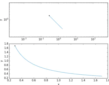
Figure 2-1: The 𝑥-𝑦 feasibility set of a simple monomial equality.

minimize 𝑥

subject to 𝑥 + 𝑦 ≤ 2, 𝑥𝑦 = 1 2

We can draw the feasibility set of the above problem in both linear and log-space, as shown in Figure 2-1. One expects that, given only two variables related through an equality and bounded by an inequality, the feasibility space is a finite line segment in log-space, and a finite exponential function in linear space. The black dot in Figure 2-1 is the global optimum of the feasibility set (𝑥 = 1 − _√1

2, 𝑦 = 1 + 1 √

2).

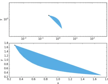
However, if we had decided to impose 𝑥𝑦 ≥ 1

2 instead of 𝑥𝑦 = 1

2, we would get a

new feasibility set as shown in Figure 2-2. Using the GP form, we can always upper-bound posynomials, and lower-upper-bound both posynomials and monomials to get convex feasible sets. Note that the optimal point, which is at 𝑥 = 1 − _√1

2, 𝑦 = 1 + 1 √

2, does

not change when the monomial equality is relaxed. This key observation will allow us to turn the equalities in most physical models into GP-compatible posynomial inequalities. The posynomial equality relaxation is explained in greater detail in [6].

However if we convert the monomial equality to 𝑥𝑦 ≤ 1

2, we will get an unbounded

model, whose feasibility set is shown in Figure 2-3. Since minimizing 𝑥 is our objective, and both variables are only upper-bounded, they both collapse towards numerical

pre-Figure 2-2: The 𝑥-𝑦 feasibility set of lower-bounding monomial, and upper-bounding posynomial.

cision zero, giving the vanishing feasibility set shown in Figure 2-3. This section will demonstrate methods to create GP-compatible models that are adequately bounded to avoid such singularities towards zero or infinity, which for the most part do not exist in real physical models. The models will be created within GPkit [3].

Figure 2-3: The 𝑥-𝑦 feasibility set of upper-bounding monomial, and upper-bounding posynomial.

2.2 Defining the design problem

GPs are amenable to solving a large variety of design problems (see [1] for an ex-tensive number of examples). This thesis uses aircraft design to demonstrate design methodologies for convex optimization since the author’s background is in aerospace engineering. Aircraft epitomize the nature of complex engineering problems. The physical relations describing their motion are nonlinear, and all of their subsystems are coupled through the primary forces in flight (thrust, weight, lift, drag). The goal of the aircraft in question will be to perform a basic ‘ferry’ mission, that is to carry a given payload over a distance while minimizing an objective function.

2.2.1 Objective functions

Objective functions are the way that a designer puts pressure on the variables in an optimization problem. To begin with, we will consider total fuel weight 𝑊𝑓 as

our objective, which will put downward pressure on all of the variables that would cause greater fuel burn, namely drag and weight. We must necessarily lower-bound all variables in the objective function that have positive exponents, and upper-bound all variables with negative exponents.

In many design problems formulated as GPs, many different objectives will put pressure on design in the same direction. For example, an aircraft optimized for fuel weight will look different compared to one that has been designed for total weight or payload-fuel consumption2_{, but each of these objectives will put a downward pressure}

on drag and weight. As such, this model will be able to take in a number of objective functions and be properly constrained and bounded. According to Raymer, an im-portant principle of aircraft design is ‘that there is no such thing as a free lunch!’ [16, pg.26]. An improvement in one objective function will result in reduced performance with respect to others.

2_{Payload-fuel consumption is the ratio of fuel weight to payload weight, a useful efficiency} pa-rameter.

2.2.2 Functional description: constraining the problem

The typical process for designing anything usually involves doing either a component decomposition or a functional decomposition of the problem. In this case, we will think about the functional decomposition to create a basic list of constraints that our aircraft will need to satisfy to be able to capture the tradeoffs in an aircraft design problem. (In Section 3.1.3, we will examine how the component decomposition can help structure larger problems.)

What does an aircraft need to be able to do to deliver payload over a distance?

ˆ It will need to sustain steady level flight, keeping itself and the payload aloft (Section 2.3.1).

ˆ It will need to overcome drag (Section 2.3.3).

ˆ It will need to contain enough fuel to complete its mission (Section 2.4.1).

ˆ It will need to sustain its structural loads (Section 2.4.3).

Note that these are in no way presented in order of importance, which is reflective of the non-hierarchical nature of GPs. In the basic example, we will choose not to model engines, and leave this as an exercise to complete in Section 3.1 to improve the model.

2.3 GP modeling from physics

Optimization model creation often starts haphazardly, with the designer having a vague idea about the set of physics that govern a problem, and some basic assumptions about the configuration. In this section, we will generate variables and constraints with abandon, and think about how to make sure each variable is adequately bounded later. Each subsection is intended to introduce the reader to an important aspect of GP modeling, accompanied by examples in implementation.

2.3.1 Free and fixed variables: weight and lift model

For this particular design problem, we start by modeling weight and lift, since one of the fundamental functions of the aircraft is to stay aloft. The aircraft has weight, which consists of the payload, wing, and fuel weights.

𝑊 ≥ 𝑊𝑝+ 𝑊𝑤+ 𝑊𝑓 (2.1)

Note that we have already had to make determination about the relation between the two sides of the equation. Heavier aircraft burn more fuel, so we are justified to put total weight as greater than the sum of the component weights since 𝑊 will be pressured downward by the objective. Furthermore, we can always add more weight to the aircraft by adding ballast to it, even if this would likely worsen the objective. So we allow for slackness in this constraint, even if we know intuitively that it will almost always be tight as explained in Section 2.2.1.

The aircraft has to sustain steady level flight, so it needs to generate enough lift. We use the naive lift is greater than weight (𝐿 ≥ 𝑊 ) model below for steady level flight:

1 2𝜌𝑉

2_𝑆𝐶

𝐿 ≥ 𝑊𝑝+ 𝑊𝑤+ 0.5𝑊𝑓 (2.2)

where the lift of the aircraft is equal to weight of the aircraft with half-fuel, which is a crude estimate of the average weight of the aircraft throughout the flight. Again, the GP form is seamless here, since lift is related to induced drag, and so it is pressured downward into the posynomial on the right hand side (RHS) of the equation.

We would also like the fully-fueled aircraft to be able to fly at a minimum speed of 𝑉𝑚𝑖𝑛 without stalling, so we add the following constraint:

𝑊 ≤ 1 2𝜌𝑉

2

𝑚𝑖𝑛𝑆𝐶𝐿𝑚𝑎𝑥 (2.3)

Note that, although we could use a monomial equality here, we don’t, because this relation does not need to be tight. It is acceptable that the aircraft is able to fly

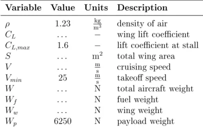
Variable Value Units Description 𝜌 1.23 _mkg3 density of air

𝐶𝐿 . . . − wing lift coefficient

𝐶𝐿,𝑚𝑎𝑥 1.6 − lift coefficient at stall

𝑆 . . . m2 total wing area

𝑉 . . . m

s cruising speed

𝑉𝑚𝑖𝑛 25 m_s takeoff speed

𝑊 . . . N total aircraft weight 𝑊𝑓 . . . N fuel weight

𝑊𝑤 . . . N wing weight

𝑊𝑝 6250 N payload weight

Table 2.1: Variables introduced in the weight and lift model.

at a velocity slower than 𝑉𝑚𝑖𝑛 for a given objective function.

At this point, we have introduced a large set of variables, some of which are input parameters, and the others free variables. The decision of whether to keep variables free or fixed can shape the model development process in all forms of optimization. The decision can be influenced by many factors in a GP, with four in particular that stand out in this model. We set the lift coefficient and takeoff speed to be constants since (I) we would need more detailed modeling to determine their values. Payload weight is set because (II) it would always be unbounded towards zero due to the downward pressure from the objective. A designer may also fix variables (III) if he/she knows their values with certainty (e.g. gravitational acceleration 𝑔) or (IV) the variable is a normalizing coefficient (which we will see in Section 3.1.2). The variables have been defined in Table 2.1, where the fixed variables have associated values. The remaining variables are free variables, to be optimized once the model is appropriately bounded.

Note that the atmospheric density 𝜌 in Table 2.1, and other atmospheric variables in Section 2 are set to be constant. The behavior of these variables with altitude will be modeled in more detail in Section 3.2 when we introduce an aircraft flight profile.

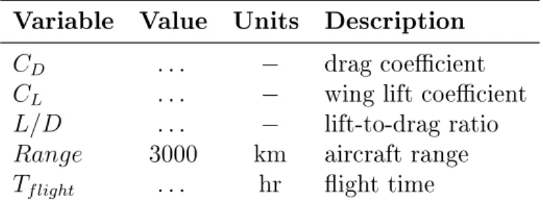
Variable Value Units Description 𝐶𝐷 . . . − drag coefficient

𝐶𝐿 . . . − wing lift coefficient

𝐿/𝐷 . . . − lift-to-drag ratio 𝑅𝑎𝑛𝑔𝑒 3000 km aircraft range 𝑇𝑓 𝑙𝑖𝑔ℎ𝑡 . . . hr flight time

Table 2.2: Variables introduced to define new performance metrics.

2.3.2 Alternate objectives: more performance metrics

As multi-objective designers, we may also be interested in knowing about additional performance metrics that can serve as part of objective functions. A few that are particularly relevant to aircraft will be introduced here.

The time of flight of the aircraft, which is a useful metric to calculate time cost, is simply the aircraft’s range divided by its cruise velocity:

𝑇𝑓 𝑙𝑖𝑔ℎ𝑡 ≥

Range

𝑉 (2.4)

The lift-to-drag ratio is also defined:

𝐿/𝐷 = 𝐶𝐿

𝐶𝐷 (2.5)

The new variables we have introduced are detailed in Table 2.2.

An important note about variables that are potential alternate objectives: these variables must always be lower-bounded (or inverted and upper-bounded) since the general GP is a minimization problem. However, if they are not also upper-bounded, these variables will likely be unbounded for a given model and run off to +∞. This means that performance-quantifying variables will need to be in a monomial form, or must be present in a posynomial objective function as shown in Equation 2.6 for boundedness. We shall see this coming into play in Section 3.2.3.

Objective ≥ 𝑛 ∑︁ 𝑖=1 𝑐𝑖 𝑛 ∏︁ 𝑖=1 𝑣𝑘𝑖,𝑗 (2.6)

2.3.3 More physics for boundedness: thrust and drag model

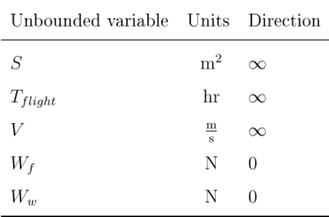
If we attempt to run our current model, we would find that it is unbounded in many variables. The results are shown in Table 2.3.

Unbounded variable Units Direction

𝑆 m2 _∞

𝑇𝑓 𝑙𝑖𝑔ℎ𝑡 hr ∞

𝑉 m_s ∞

𝑊𝑓 N 0

𝑊𝑤 N 0

Table 2.3: Unbounded variables in the weight and lift model.

This is not surprising at all, since none of the defined constraints lower-bound 𝑊𝑓, the objective function. Additionally, without pressure from the objective, any

variables that are not both upper- and lower- bounded will tend to blow up. This is in-dicative usually that more modeling or direct substitutions are required to sufficiently bound the variables.

In this case, we lack a propulsion model which would properly bound fuel weight, velocity, and time of flight. For initial modeling purposes, we assume a naive con-stant brake specific fuel consumption (BSFC) for the ‘engine’ of the aircraft, which is assumed to provide as much thrust as needed. Since 𝑇 ≥ 𝐷:

𝑊𝑓 ≥ 𝑔 × BSFC × 𝑇𝑓 𝑙𝑖𝑔ℎ𝑡× 𝐷𝑉 (2.7)

the fuel weight required is the product of gravitational acceleration, BSFC, time of flight, and the total drag power on the aircraft. The drag is the product of dynamic pressure (1

2𝜌𝑉

2_{), planform area 𝑆, and the coefficient of drag of the aircraft:}

𝐷 ≥ 1 2𝜌𝑉

2_𝑆𝐶

There are yet more relaxed monomial equalities in Equations 2.7 and 2.8. If the pressure on the left hand side (LHS) or RHS of a monomial equality are clear as in these cases, it is a good practice to relax the equality to leave as many degrees of freedom in the design space as possible. The intuition is that we can almost always spend more fuel or have more drag, but we are confident that the constraints will be tight since our objective will suffer as a consequence.

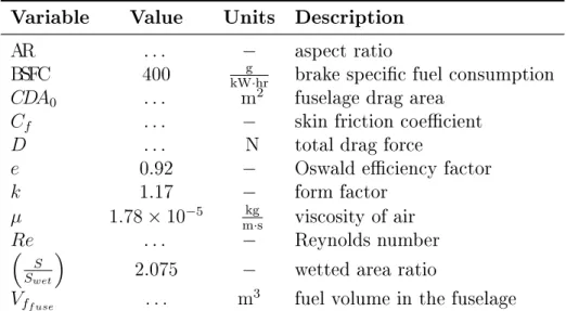
The drag coefficient of the aircraft is assumed to be the sum of the fuselage drag, the wing profile drag, and the wing induced drag coefficients [7]:

𝐶𝐷 ≥ 𝐶𝐷𝑓 𝑢𝑠𝑒+ 𝐶𝐷𝑤𝑝𝑎𝑟 + 𝐶𝐷𝑖𝑛𝑑 (2.9)

The individual components of the drag are represented as monomial equalities, borrowing constraints 2.10 through 2.15 from [7]. The fuselage drag is a function of its drag area 𝐶𝐷𝐴0 and the planform area of the wing:

𝐶𝐷𝑓 𝑢𝑠𝑒 =

𝐶𝐷𝐴0

𝑆 (2.10)

where the 𝐶𝐷𝐴0 is linearly proportional to the volume of fuel in the fuselage:

𝑉𝑓𝑓 𝑢𝑠𝑒 = 𝐶𝐷𝐴0× 10 m (2.11)

Note that we correct the dimensionality of the volume here, since GPkit automat-ically checks units.

The wing profile drag is the product of the form factor, the friction drag coefficient, and the wetted area ratio of the wing [7],

𝐶𝐷𝑤𝑝𝑎𝑟 = 𝑘𝐶𝑓𝑆𝑤𝑒𝑡𝑟𝑎𝑡𝑖𝑜 (2.12)

The Reynolds number of the aircraft wing is approximated

𝑅𝑒 ≤ 𝜌 𝜇𝑉

√︂ 𝑆

𝐴𝑅 (2.13)

Variable Value Units Description

AR . . . − aspect ratio

BSFC 400 _kW·hrg brake specific fuel consumption 𝐶𝐷𝐴0 . . . m2 fuselage drag area

𝐶𝑓 . . . − skin friction coefficient

𝐷 . . . N total drag force

𝑒 0.92 − Oswald efficiency factor

𝑘 1.17 − form factor 𝜇 1.78 × 10−5 _m·skg viscosity of air 𝑅𝑒 . . . − Reynolds number (︁ 𝑆 𝑆𝑤𝑒𝑡 )︁

2.075 − wetted area ratio

𝑉𝑓𝑓 𝑢𝑠𝑒 . . . m

3 _{fuel volume in the fuselage}

Table 2.4: Variables introduced in the thrust and drag model.

Unbounded variable Units Direction

𝑉𝑓𝑓 𝑢𝑠𝑒 m

3 ₀

𝑊𝑤 N 0

Table 2.5: Unbounded variables in the GP-compatible formulation.

assuming a turbulent flat plate flow:

𝐶𝑓 ≥

0.074

𝑅𝑒0.2 (2.14)

The induced drag of the wing is calculated with a span efficiency factor 𝑒, and is a function of the 𝐶𝐿 and aspect ratio AR of the wing.

𝐶𝐷𝑖𝑛𝑑𝑢𝑐𝑒𝑑 =

𝐶2 𝐿

𝜋𝐴𝑅𝑒 (2.15)

The new variables are detailed in Table 2.4.

As shown in Table 2.5, attempting to run the model as is results in both the fuselage fuel volume 𝑉𝑓𝑓 𝑢𝑠𝑒 and the wing weight 𝑊𝑤 still having no lower bounds.

2.4 Limits of GP and convexity, and SP modeling

Even with the demonstrated strengths of GPs in solving certain classes of problems, it is important to recognize that the mathematical framework has limits. The three distinct types of GP-incompatibility in design problems are detailed by Hoburg [6], which are discreteness, quasi-convexity, and multi-modality. Discreteness in the GP can be approached by coupling discrete programming methods such as branch-and-bound into a sequential GP. This is outside of the scope of this thesis. Quasi-convexity and to a certain extent multimodality can be addressed through a non-log-convex ex-tension of GPs called SPs, where certain constraints are expressed as signomial (or difference-of-posynomial) constraints (described in greater detail in Appendix A.2). Even the addition of a single signomial constraint turns the problem from a GP to a SP, which means that the problems loses convexity and all of the mathematical guar-antees associated with it. It takes engineering intuition to recognize where and when improved modeling is worth the loss of the mathematical guarantees. Kirschen [10] describes in greater detail how signomial constraints are often required to capture fundamental design tradeoffs.

2.4.1 Signomial constraints: fuel volume model

In an attempt to put a lower bound 𝑉𝑓𝑓 𝑢𝑠𝑒, we will be adding a fuel volume model

to SimPleAC, where fuel can be stored in the wing or in the fuselage. The fuel volume will be modeled first instead of the wing weight because the wing weight will be a function of the fuel stored in the fuselage. The reason why this model is GP-incompatible is because of the following constraint which follows logically:

𝑉𝑓𝑎𝑣𝑎𝑖𝑙 ≤ 𝑉𝑓𝑤𝑖𝑛𝑔 + 𝑉𝑓𝑓 𝑢𝑠𝑒 (2.16)

The fuel volume available must be less than the sum of the fuel volume available in the wing and the fuselage. It turns out that volumes that ‘contain’ free variables can create signomial constraints. (One way around this is potentially creating fuel fraction variables to denote how much fuel is stored in each volume, but other potential

parametrizations will not be explored here.)

As such, we can continue to develop the model, since it is important for us to capture the fuel distribution between the wing and the fuselage. Fuel weight is going to influence the lift required of the aircraft, so the weight of the fuel is determined using a density parameter 𝜌𝑓.

𝑉𝑓 =

𝑊𝑓

𝜌𝑓𝑔

(2.17)

We need a model of how much fuel volume there is in a wing. Intuitively, we would expect the volume within a wing to be related linearly to its thickness ratio (𝜏) and span (𝑏), and to the square of its chord (𝑐).

𝑉𝑓𝑤𝑖𝑛𝑔 ∝ 𝜏 𝑏𝑐

2 _(2.18)

It is convenient to express relation 2.18 in terms of planform area 𝑆, aspect ratio AR and thickness ratio 𝜏 only. Using the additional relations 𝐴𝑅 = 𝑏2

𝑆 and 𝑆 ∝ 𝑏𝑐, we can express 𝑉𝑓𝑤𝑖𝑛𝑔. 𝑉𝑓𝑤𝑖𝑛𝑔 ∝ 𝜏 (︂ 𝐴𝑅 𝑆 )︂0.5_{(︂ 𝑆} 𝑏 )︂2 ∝(︂ 𝐴𝑅 𝑆 )︂0.5 𝑆2 𝑆𝐴𝑅 ∝ √ 𝑆𝜏 √ 𝐴𝑅 (2.19) 𝑉_𝑓2_{𝑤𝑖𝑛𝑔} ≤ 9 × 10−4 m4×𝑆𝜏 2 𝐴𝑅 (2.20)

Such variable transformations can be useful to have a minimal parametrization of designs. One can solve the minimal optimization problem, and post-process the solution of the problem to get a complete geometry as necessary. The new variables introduced to bound fuel volume are in Table 2.6. (In Equation 2.20, the constant 9 × 10−4 m4 was picked as the coefficient in front of the relation by tuning it after the

Variable Value Units Description 𝜌𝑓 817 _mkg3 density of fuel

𝑔 9.81 m

s2 gravitational acceleration

𝜏 0.12 − airfoil thickness to chord ratio 𝑉𝑓 . . . m3 fuel volume

𝑉𝑓𝑎𝑣𝑎𝑖𝑙 . . . m

3 _{fuel volume available}

𝑉𝑓𝑤𝑖𝑛𝑔 . . . m

3 _{fuel volume in the wing}

Table 2.6: Variables introduced in the fuel model.

2.4.2 Arguments for the signomial equality

This segue will explain and motivate the use of signomial equalities, as described in [15], in SP modeling. Signomial equalities must be used as a last resort. The signomial equality is the only place where the feasibility set of individual GPs within a SP solve are not guaranteed to be subsets of the feasibility set of the SP. This is because the signomial solution algorithm in GPkit flattens the original signomial equality constraint, a concave curve in space in 𝑛-dimensions, onto a line in log-space in 𝑛-dimensions(Method C in [15]) that intersects the original constraint at the optimal point of the last GP solve. This is undesirable, although the final solution of the SP with equalities is guaranteed to be in the feasibility region of the SP. Furthermore, SPs with signomial equalities have been demonstrated to require more GP solves than SPs without signomial equalities. However, there are a few arguments to be made in defense of signomial equalities.

One good use case of the signomial equality is in constraints in which the direction of pressure on free variables is not clear. This ensures the tightness of constraints that may otherwise have unbounded variables. A good example is in atmospheric models. Although the pressure on air viscosity 𝜇 is almost certainly downward since it results in lower drag, the pressure on air density 𝜌 is not clear because of the tradeoffs between aircraft endurance and range.

The second reason is that we are not interested in the ‘feasibility set’ of the at-mosphere, since this has no intuition behind it: at every altitude, the atmospheric quantities can only be be represented by single quantities. Additionally, the

com-putational penalty of implementing signomial equalities in atmospheric models is low, since the monomial approximation to the atmospheric data is not far from the monomial approximations made to the signomial equality. In fact, when we add an atmospheric model to SimPleAC in Section 3.2, we will be implementing signomial equalities to represent both air density 𝜌 and viscosity 𝜇.

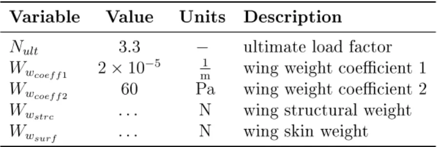
2.4.3 Completing the model: wing structural model

Only one unbounded variable remains, which is wing weight 𝑊𝑤. We can think of

wing weight as having two components, the skin weight that only grows as a function of wing area and the structural weight which is a function of both the geometry and loading. The surface weight expression is straightforward.

𝑊𝑤𝑠𝑢𝑟𝑓 ≥ 𝑊𝑤𝑐𝑜𝑒𝑓 𝑓 2𝑆 (2.21)

We would like wing structural weight to account for the loading distribution and the geometry of the wing. The wing will have to sustain a maximum bending load (we will neglect shear, since the two are coupled) due to maximum takeoff weight, multiplied by an ultimate structural factor 𝑁𝑢𝑙𝑡for maneuvering. I have borrowed the

wing weight model from [7], and adapted it through a structural weight coefficient 𝑊𝑤𝑐𝑜𝑒𝑓 𝑓 1. Note that this equation captures the major trends in wing structural sizing.

We can see this through looking at the partial derivatives of the wing weight with respect to the different free variables. The weight grows with the cube of the span (𝐴𝑅1.5 ₌ 𝑏3

𝑆1.5

𝑐𝑜𝑛𝑠𝑡𝑎𝑛𝑡, derived from the integration of a quadratically increasing bending

moment), linearly with the maximum structural factor 𝑁𝑢𝑙𝑡, and inversely with the

surface area3_{. Using similar partial-derivative based analyses, it is often easy to make}

first-order models for components.

𝑊𝑤𝑠𝑡𝑟𝑐 ≥

𝑊𝑤𝑐𝑜𝑒𝑓 𝑓 1

𝜏 𝑁𝑢𝑙𝑡𝐴𝑅

1.5√︁_(𝑊

0+ 𝜌𝑓𝑔𝑉𝑓𝑓 𝑢𝑠𝑒)𝑊 𝑆 (2.22)

3_{This can be difficult to see, but since 𝑆 ∝ 𝑏𝑐𝑜𝑛𝑠𝑡𝑎𝑛𝑡𝑐 and loading is constant, as area grows, the} thickness of the wing grows as well at a constant 𝜏. So the weight increases linearly with S, and stiffness increases with the cube of S. Integrated over the whole wing this yields a 𝑆−1 _relation.

Variable Value Units Description

𝑁𝑢𝑙𝑡 3.3 − ultimate load factor

𝑊𝑤𝑐𝑜𝑒𝑓 𝑓 1 2 × 10

−5 1

m wing weight coefficient 1

𝑊𝑤𝑐𝑜𝑒𝑓 𝑓 2 60 Pa wing weight coefficient 2

𝑊𝑤𝑠𝑡𝑟𝑐 . . . N wing structural weight

𝑊𝑤𝑠𝑢𝑟𝑓 . . . N wing skin weight

Table 2.7: Variables introduced in the wing structural model.

Equation 2.22 takes into account the root bending moment relief due to presence of fuel and weight in the wings by performing a geometric average of the total weight, and the weight excluding wing fuel and wing weight.

The total wing weight is now lower-bounded by its component weights, and we have introduced the final set of variables in Table 2.7.

𝑊𝑤 ≥ 𝑊𝑤𝑠𝑢𝑟𝑓 + 𝑊𝑤𝑠𝑡𝑟𝑐 (2.23)

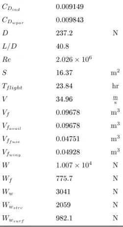
2.5 Results of SimPleAC

The benefits of convex optimization and GP in both solution quality (in terms of mathematical guarantees) and the low-cost computation of sensitivities have been detailed in ([7],[11]), so these benefits will not be featured here. However, the values of the free variables, and the sensitivities of the fixed parameters are presented for the reader.

Table 2.8: Values of free variables in the SimPleAC model.

Free Variables Value Units

(𝐶𝐷𝐴0) 0.004751 m2 𝐴 23.41 𝐶𝐷 0.01928 𝐶𝐿 0.7867 𝐶𝑓 0.004054 𝐶𝐷𝑓 𝑢𝑠𝑒 2.902 × 10 −4

𝐶𝐷𝑖𝑛𝑑 0.009149 𝐶𝐷𝑤𝑝𝑎𝑟 0.009843 𝐷 237.2 N 𝐿/𝐷 40.8 𝑅𝑒 2.026 × 106 𝑆 16.37 m2 𝑇𝑓 𝑙𝑖𝑔ℎ𝑡 23.84 hr 𝑉 34.96 m_s 𝑉𝑓 0.09678 m3 𝑉𝑓𝑎𝑣𝑎𝑖𝑙 0.09678 m 3 𝑉𝑓𝑓 𝑢𝑠𝑒 0.04751 m 3 𝑉𝑓𝑤𝑖𝑛𝑔 0.04928 m 3 𝑊 1.007 × 104 _N 𝑊𝑓 775.7 N 𝑊𝑤 3041 N 𝑊𝑤𝑠𝑡𝑟𝑐 2059 N 𝑊𝑤𝑠𝑢𝑟𝑓 982.1 N

Table 2.10: Sensitivities of parameters in the SimPleAC model.

Sensitivities Value BSFC +1.1 𝑅𝑎𝑛𝑔𝑒 +1.1 𝑊𝑝 +1.1 𝑔 +1.1 (︁ 𝑆 𝑆𝑤𝑒𝑡 )︁ +0.57 𝑘 +0.57 𝑒 -0.53 𝑉𝑚𝑖𝑛 -0.49 𝜏 -0.34 𝑁𝑢𝑙𝑡 +0.31 𝑊𝑤𝑐𝑜𝑒𝑓 𝑓 1 +0.31 𝜌 -0.3 𝐶𝐿,𝑚𝑎𝑥 -0.24

𝑊𝑤𝑐𝑜𝑒𝑓 𝑓 2 +0.15

𝜇 +0.11

Chapter 3

Extensibility of GP

Recalling from Figure 1-1, traditional gradient-based design optimization tools im-plement convergence loops that assume structure within a given design problem. The ‘bag of constraints’ form of the GP means that constraints can be added to the problem without having to restructure the optimization formulation. This property, coupled with the object-oriented modeling framework of GPkit, allows GP compatible models to be continuously extensible. This section will demonstrate common meth-ods used to extend the capability and improve the fidelity of GP- and SP-compatible models.

3.1 Modularization and improved fidelity: engine model

The aircraft currently has an engine that weighs nothing and magically supplies un-limited power. This is obviously unphysical, and requires refinement.

3.1.1 Creating an engine submodel

Before even thinking about modeling, we would like to leverage the object-oriented GPkit models to put the variables describing the engine into a submodel (currently only consisting of the BSFC variable). In the GPkit software, we do this by creating a new class (an object in the Python language) called Engine and creating a setup

method that returns the constraints within it. The Model and Variable objects in the sample code are imported from GPkit.

class Engine ( Model ):

def setup (self):

# Dimensional constants

BSFC = Variable (" BSFC ", 400 , "g /( kw*hr )",

" brake specific fuel consumption ")

constraints = []

return constraints

We allow the SimPleAC model to contain the variables and constraints of the engine as follows:

class SimPleAC ( Model ):

def setup (self):

self. engine = Engine ()

self. components = [self. engine ] ...

return constraints , self. components

This restructuring of the model yields the exact same GP formulation as the unstructured problem, but gives us the flexibility to develop submodels collaboratively and in a disciplined manner.

If we think of an engine as an input-output system, we can determine how it would interact with the SimPleAC system, and create appropriately bounded sets of variables. At the most basic level, an engine provides shaft power, consumes fuel, and has weight. The model is missing both the shaft power and weight description of the engine. If we abstract away the propeller (the relation between shaft power and thrust power) through a propeller efficiency, we can perhaps relate maximum power to weight.

3.1.2 Data-based modeling: engine power vs. weight

We can imagine that, for a specific kind of engine, there is a relation between the maximum shaft power available and the mass of the engine, somewhat related to the cube-square law, which describes the relation between the surface area and volume of objects. And let’s assume that our knowledge of the internal workings of engines is limited, but we have some knowledge of the technology available in the market and have data to support it. Using GPfit [8], we will try to fit the data to find GP compatible relations between engine weight and maximum power. This section will try to highlight the best practices when making data-based models.

To be able to fit the engine power versus weight data, we take several important steps.

ˆ Comb the data. Since we are essentially projecting data with potentially high standard deviation onto a single line, it is important to fit the ranges of data we care about.

ˆ Normalize the data. Normalizing the data by some known quantity is prefer-able, since fits should not be dependent on the units that are used while perform-ing it. This also helps the fit integrate seamlessly into GPkit, since dimensional fits would require units manipulation to avoid errors. The data can be normal-ized by reference quantities (in this case using the maximum power and weight values from the data set).

ˆ Choose the type of fit. In [8], affine (SMA) and implicit softmax-affine (ISMA) functions are proposed and implemented as convex approxima-tions to data. Depending on the behavior of the data, one or the other may be appropriate. For engineering relations that are expected to be smooth, SMA functions are often good approximations. However, if kinks are expected in the functions, ISMA functions can locally adjust the softness of the fit to reduce the error of the fit.

posynomial terms can be changed to better capture the trends in the data. RMS error can be reduced by including more posynomial terms, but only if the variable of interest has downward pressure on it from the objective function (since it is on the greater side of the inequality). Otherwise fits are limited to monomial equalities in 𝑛-dimensions.

After having performed these intermediate steps on the engine data, the relation we obtain for the one-term (monomial) approximation is as follows:

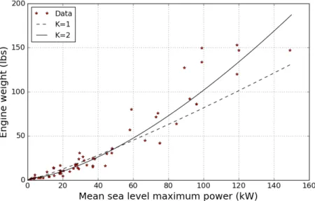
(︂ 𝑊𝑒𝑛𝑔 𝑊𝑒𝑛𝑔,𝑚𝑎𝑥 )︂0.100 = 0.988 (︂ 𝑃𝑠ℎ𝑎𝑓 𝑡 𝑃𝑠ℎ𝑎𝑓 𝑡,𝑚𝑎𝑥 )︂0.117 (3.1) This fit, shown by the dashed line in Figure 3-1, has a root mean square error of 0.414, which has to do both with the quality of the fit and the level of variation in the data. Since engine weight will have downward pressure on it from the objective function, we can easily use a two-term posynomial approximation to improve its error.

Figure 3-1: Engine MSL power versus weight fits for 𝐾 = 1, 2 posynomial terms with underlying data. (︂ 𝑊𝑒𝑛𝑔 𝑊𝑒𝑛𝑔,𝑚𝑎𝑥 )︂1.92 ≥ 4.41 × 10−3 (︂ 𝑃𝑠ℎ𝑎𝑓 𝑡 𝑃𝑠ℎ𝑎𝑓 𝑡,𝑚𝑎𝑥 )︂0.759 + 1.44 (︂ 𝑃𝑠ℎ𝑎𝑓 𝑡 𝑃𝑠ℎ𝑎𝑓 𝑡,𝑚𝑎𝑥 )︂2.90 (3.2)

This relation has an RMS error of 0.346, which is a significant improvement. Both fits are shown with the data in Figure 3-1 for comparison.

With a SMA approximation, adding more than two terms to the fit do not improve its RMS error on the given data, due to the large standard deviation of the data used. As such, we will proceed with the 2-term posynomial fit.

Other constraints in engine model

The cruise shaft power is constrained to be 20% of the maximum shaft power of the engine, to account for engine surge power demands and add engineering realism. This rather arbitrary constraint is removed later when the full mission model is integrated.

𝑃𝑠ℎ𝑎𝑓 𝑡 ≤

1

5𝑃𝑠ℎ𝑎𝑓 𝑡,𝑚𝑎𝑥 (3.3)

3.1.3 Converting all subsystems into submodels

Within this framework, we can modularize the SimPleAC into wing and fuselage modules as well, with very little additional work. This creates the variable and constraint hierarchy as presented in Figure 3-2, which define all of the constraints required for SimPleAC to fly one flight segment.

Aircraft

Wing Fuselage Engine

Figure 3-2: Variable and constraint hierarchy of the SimPleAC model for a single flight segment.

Uni-directional graph structures such as in Figure 3-2 are informative, since they provide an intuitive representation of the way constraints and variables are passed between GPkit models. In this basic framework, variables and constraints from one model can only be called by models that are higher and connected in the diagram. This reconciles the fact that object creation in software engineering is serial, whereas the components of the system being optimized are interconnected. The way the SP

is solved at the end has no hierarchy, but as we will see in Section 3.2 a hierarchi-cal representation will facilitate the vectorization of constraints required for mission design.

3.2 Mission design and performance modeling form

The SimPleAC defined so far works well to demonstrate the capabilities of SPs in helping explore tradeoffs in engineering design. However, often in the design process, we will want to test the performance of a design in different conditions, and/or during different phases of a mission. This requires the vectorization of constraints that relate to the performance of the design. What we’d like to do is to have a single aircraft optimize both its static sizing variables (having to do with the airframe), and its flight performance simultaneously. This requires a major augmentation of the model graph defined in Figure 3-2, into a uni-directional graph as shown in Figure 3-3.

Mission Aircraft Perf. Wing Perf. Atmosphere Engine Perf. Aircraft

Wing Fuselage Engine

Aircraft Perf. Wing Perf. Atmosphere Engine Perf. Segment 2 Segment 1

Figure 3-3: Variable and constraint hierarchy of the SimPleAC static+performance model for two flight segments. Models that include sizing variables are bolded while models that include performance variables are italicized. There are models that con-tain both kinds of variables.

Figure 3-3 represents a model with two flight segments, where the models enclosed in rectangles contain the set of constraints that are vectorized by the number of flight segments, 𝑁𝑠𝑒𝑔𝑚𝑒𝑛𝑡𝑠 = 2. Each one of the performance models contains variables that

change between flight segments. Note that the fuselage is the only subcomponent not to have a performance model. This is because the drag coefficient of the fuselage is

assumed to be constant between flight segments, making it static. A Mission model that links flight segments together has been added, as well as an Atmosphere model, which describes the conditions in which the aircraft operates.

The static aircraft model and the atmospheric state are passed as arguments to multiple performance models within this framework. To transform our previously static model to the performance-static model hierarchy we have identified, we have to determine which variables belong in which node of the graph. Table 3.1 details the full decomposition of the model into its submodels in the format defined by Figure 3-3. This is as simple as identifying which variables we do not expect to change during flight segments, and which ones we do. Note that some of the variables from the previous sections have been renamed (e.g. 𝑇𝑓 𝑙𝑖𝑔ℎ𝑡 → 𝑡𝑚 and 𝑊𝑓 → 𝑊𝑓𝑚) to clarify

their purpose within this framework.

Table 3.1: Variables of SimPleAC in static+performance modeling, detailed in the variable and constraint hierarchy.

Variable Units Description Mission

𝐶 _hr1 hourly cost index

𝑊𝑓𝑚 N total mission fuel

𝑡𝑚 hr total mission time

𝑅𝑎𝑛𝑔𝑒 km aircraft range

𝑊𝑝 N payload weight

𝑡𝑠 hr segment time

𝑅𝑠 km segment range

𝑊𝑓𝑠 N segment fuel burn

𝑊𝑠𝑡𝑎𝑟𝑡 N segment beginning weight

𝑊𝑎𝑣𝑔 N segment average weight

𝑊𝑒𝑛𝑑 N segment end weight

𝑑ℎ 𝑑𝑡 m hr climb rate ℎ m flight altitude 𝑉𝑚𝑖𝑛 m_s takeoff speed Mission/Atmosphere 𝜇 _(m·s)kg dynamic viscosity

𝜇𝑀 𝑆𝐿 _(m·s)kg dynamic viscosity at MSL

𝜌 _mkg3 density of air

𝜌𝑀 𝑆𝐿 _mkg3 density of air at MSL

ℎ m altitude

ℎ𝑡𝑜𝑝 m highest altitude valid Mission/SimPleAC

𝑉𝑓 m3 maximum fuel volume

𝑉𝑓𝑎𝑣𝑎𝑖𝑙 m

3 _{fuel volume available}

𝑊 N maximum takeoff weight

𝑊𝑓 N maximum fuel weight

𝑔 _sm2 gravitational acceleration

𝜌𝑓 _mkg3 density of fuel

Mission/SimPleAC/Engine

𝑃𝑠ℎ𝑎𝑓 𝑡,𝑚𝑎𝑥 kW MSL maximum shaft power

𝑃𝑠ℎ𝑎𝑓 𝑡,𝑟𝑒𝑓 kW reference MSL maximum shaft power

𝑊𝑒 N engine weight

𝑊𝑒,𝑟𝑒𝑓 N reference engine weight

𝜂𝑝𝑟𝑜𝑝 propeller efficiency

Mission/SimPleAC/Fuselage

(𝐶𝐷𝐴0) m2 _{fuselage drag area}

𝐶𝐷𝑓 𝑢𝑠𝑒 fuselage drag coefficient

𝑉𝑓𝑓 𝑢𝑠𝑒 m

3 _{fuel volume in the fuselage} Mission/SimPleAC/Wing

𝐴 aspect ratio

𝑆 m2 _{total wing area}

(︁ 𝑆 𝑆𝑤𝑒𝑡

)︁

wetted area ratio

𝑉𝑓𝑤𝑖𝑛𝑔 m

3 _{fuel volume in the wing}

𝑊𝑤 N wing weight

𝑊𝑤𝑠𝑡𝑟𝑐 N wing structural weight

𝑊𝑤𝑠𝑢𝑟𝑓 N wing skin weight

𝑁𝑢𝑙𝑡 ultimate load factor

𝑊𝑤𝑐𝑜𝑒𝑓 𝑓 1

1

m wing weight coefficient 1 𝑊𝑤𝑐𝑜𝑒𝑓 𝑓 2 Pa wing weight coefficient 2

𝐶𝐿,𝑚𝑎𝑥 lift coefficient at stall

𝑘 form factor

𝜏 airfoil thickness to chord ratio Mission/SimPleACP

𝐶𝐷 drag coefficient

𝐷 N total drag force

𝐿/𝐷 lift-to-drag ratio

𝑅𝑒 Reynolds number

𝑉 m

s cruising speed Mission/SimPleACP/EngineP

BSFC _(hr·kW)g brake specific fuel consumption

𝑃𝑠ℎ𝑎𝑓 𝑡 kW shaft power

𝑇 N propeller thrust

Mission/SimPleACP/WingP

𝐶𝐿 wing lift coefficient

𝐶𝑓 skin friction coefficient

𝐶𝐷𝑖𝑛𝑑 wing induced drag

𝐶𝐷𝑤𝑝𝑎𝑟 wing profile drag

Then, using the variable structure in Table 3.1, we can place the constraints in the appropriate locations. Each constraint should be placed in the model that contains the variable in the constraint that is highest in the level of hierarchy. For example, we can consider the constraint for thrust power in Equation 3.4.

𝑇 × 𝑉 ≤ 𝜂𝑝𝑟𝑜𝑝𝑃𝑠ℎ𝑎𝑓 𝑡 (3.4)

We expect that thrust (𝑇 ) and shaft power (𝑃𝑠ℎ𝑎𝑓 𝑡) variables exist in Engine

Per-formance. Since our model has no model for propeller efficiency (𝜂𝑝𝑟𝑜𝑝), we treat it

as a static parameter in Engine. Velocity (𝑉 ) is a variable in Aircraft Perfor-mance. As a result, the constraint for thrust power would logically reside in the Aircraft Performance model, the highest level in the hierarchy as shown in Fig-ure 3-4. Since this model is vectorized, the constraint would be vectorized by the number of flight segments we create.

Mission Aircraft Perf. Wing Perf. Atmosphere Engine Perf. Aircraft

Wing Fuselage Engine Segment

Figure 3-4: Variable hierarchy of thrust constraint 3.4. The models that contain the variables in the constraint are enclosed in circles. Constraint logically resides in Aircraft Perf.. The vectorization of flight segment performance models in the rectangle has been neglected for clarity.

amenable to vectorization and mission design.

3.2.1 Linking performance models: flight segments

Although the variables in the performance models are vectorized, they can be con-strained against each other. If each of the Aircraft Performance models were operating independently of each other simulating different missions, then they would simply be merged in the bag of constraints of Mission. However, we know that the models are related since the aircraft burns fuel throughout the mission, changing its flight characteristics.

The derivation of the SP-compatible flight segment models has been detailed in [11], and used widely within the CEG in aircraft design. It defines segment start, end and average weights, as well as altitude, and all of its relevant constraints are contained in the Mission model. Please find the full set of variables belonging to the flight segment model in Appendix B.1.

ℎ𝑎𝑣𝑔1 = 1 2∆ℎ1 (3.5) ℎ𝑎𝑣𝑔𝑖 = √︀ ℎ𝑖× ℎ𝑖−1, 𝑖 = 2, ..., 𝑁𝑠𝑒𝑔𝑚𝑒𝑛𝑡𝑠 (3.6)

to define an average altitude variable ℎ𝑎𝑣𝑔 with respect to the segment altitude

change variable ∆ℎ and segment ending altitude ℎ in Section 3.2.2. This adds con-servatism to the density and drag (otherwise, the air density for a flight segment is calculated at the end of the segment, at which the aircraft is at its highest altitude). The cruise altitude (final altitude in every flight segment but the initial segment) has been constrained to be greater than 5000m.

As with most GP approximations, there are limitations to this model. To avoid non-positive altitude change values (∆ℎ), we restrict the aircraft to climb during every segment, and don’t model descents. Furthermore, we have binned the flight segments to equal range segments to avoid the potential lower-unboundedness of the lengths of certain segments.

3.2.2 Characterizing the environment: atmospheric model

We have created a mission and flight segment framework without having a model of the environment in which the aircraft operates. So far, we have assumed that the aircraft flies at a constant altitude (sea level) for a single mission segment, and is subject to the same air density and viscosity. An atmospheric model is essential to capturing the tradeoffs between flight altitude, engine performance, and lift and drag characteristics. This simplification is overcome through vectorization.

Tao’s atmosphere fits [17] have been borrowed for this purpose. These are 2-term softmax-affine fits of the atmospheric quantities of interest (𝜌 and 𝜇 in this thesis) with respect to altitude. The constraints are guaranteed to be tight through signomial equalities, as explained in Section 2.4.2. The relations are valid between 0-10000m of altitude.

environmental variables are inextricably coupled to performance. Another good ex-ample of environmental modeling in GP is performed by Burton [4], where wind speeds are integrated into a loitering aircraft optimization problem.

3.2.3 Mission objectives

Recalling from Section 2.3.2, upper-unbounded performance metrics often have to reside in the objective function to be bounded. We combine mission fuel 𝑊𝑓𝑚 and

mission time 𝑡𝑚into a composite objective function through a cost index 𝐶 for

bound-edness,

Objective ≥ 𝑊𝑓

1

N + C × 𝑡𝑚 (3.7)

and divide 𝑊𝑓𝑚 by newtons to achieve uniform units (non-dimensional). Another

method to achieve proper boundedness is to add an arbitrary large upper bound. However this will result in the bounding constraint being tight and giving unphysical results, and so this thesis will implement the objective in Equation 3.7 instead. Cost index C is defined as a separate parameter so that we can observe the sensitivity of the variable post-optimization.

3.3 Design exploration through mission design

There are a few interesting methods that we can use to explore potential designs using GPs. So instead of showing the optimum of the SimPleAC for a single mission, leveraging the speed of convex optimization, we can map out the entire design space with respect to mission parameters. Please refer to [9] for details on the computational advantages of the GP and SP compared to other non-linear optimization methods.

In this case, the SimPleAC has been optimized (for 𝑁𝑠𝑒𝑔𝑚𝑒𝑛𝑡𝑠= 4) over a range of

payload weight (1000-10000 N) and range (1000-5000km), and the mission fuel weight and total weight have been plotted in contour plots in Figure 3-5. Note that every point in the design space represents a fully optimized aircraft. The full list of inputs

Constants Value Units Description 𝑅𝑎𝑛𝑔𝑒 [1000-10000] km aircraft range 𝑊𝑝 [1000-5000] N payload weight

𝐶 120 _hr1 hourly cost index 𝑇 /𝑂𝑓 𝑎𝑐𝑡𝑜𝑟 2 takeoff thrust factor 𝑉𝑚𝑖𝑛 25 m_s takeoff speed

ℎ𝑐𝑟𝑢𝑖𝑠𝑒 5000 m minimum cruise altitude

Table 3.3: Inputs to the design space exploration of the Mission model.

Figure 3-5: The fuel and total weight contours with respect to range and payload.

to the Mission model are detailed in Table 3.3

In Section 2.4.1 we had to weigh whether or not it was worth losing the math-ematical guarantees of convexity to be able to model fuel storage. Now we can use our SP model to understand the tradeoffs in fuel storage, and when it is beneficial to store fuel in the wing versus the fuselage.

Figure 3-6 shows how designs for different range and payload requirements allocate fuel differently within the aircraft. As the mission range increases for a given payload weight (upward movement on the graph), more and more fuel is allocated within the fuselage as a proportion of total fuel. Since fuselage fuel volume is directly related to increased fuselage drag, it is logical that no fuel is put in the fuselage until the fuel volume constraint in the wing becomes tight. And this is the behavior that is observed, since no fuel is allocated in the fuselage towards the lower right of the graph. For composite objective functions, it can be difficult to have intuitions about how sensitivities to parameters can affect the design, since the parameters act on multiple

Figure 3-6: Fraction of total fuel stored in fuselage with respect to range and payload.

Figure 3-7: Time cost and time cost index sensitivity contours. We can gain intu-ition about the relative importance of different components of composite objective functions by showing both the costs and their sensitivities together.

variables of interest. A way to attempt to decouple these is to plot both the cost of a variable in the objective and its relevant sensitivity next to each other, as shown in Figure 3-7. Taking a look at point [4000N,3500km], we can follow the time cost (2 × 103) contour to see all of the missions with the same time cost as this mission

(same average flight speed), and see how the fraction of time cost versus total cost varies through the sensitivity to the time cost index. This can help a designer gain intuition about the relative importance of different components of cost.

Variable/Model Sensitivity Variable description Mission

𝑅𝑎𝑛𝑔𝑒 +1.1 aircraft range

𝑉𝑚𝑖𝑛 -0.67 takeoff speed

𝐶 +0.46 hourly cost index

𝑊𝑝 +0.45 payload weight

ℎ𝑐𝑟𝑢𝑖𝑠𝑒 +0.12 minimum cruise altitude

Mission/SimPleAC

𝑔 +0.54 gravitational acceleration

𝜌𝑓 -0.042 density of fuel

Mission/SimPleAC/Engine

𝜂𝑝𝑟𝑜𝑝 -0.65 propeller efficiency

𝑃𝑠ℎ𝑎𝑓 𝑡,𝑟𝑒𝑓 -0.067 reference MSL maximum shaft power

𝑊𝑒,𝑟𝑒𝑓 +0.044 reference engine weight

Mission/SimPleAC/Wing (_𝑆𝑆

𝑤𝑒𝑡) +0.45 wetted area ratio

𝑘 +0.45 form factor

𝐶𝐿,𝑚𝑎𝑥 -0.33 lift coefficient at stall

𝑒 -0.17 Oswald efficiency factor

𝑊𝑤𝑐𝑜𝑒𝑓 𝑓 2 +0.12 wing weight coefficient 2

𝜏 -0.11 airfoil thickness to chord ratio

𝑁𝑢𝑙𝑡 +0.07 ultimate load factor

𝑊𝑤𝑐𝑜𝑒𝑓 𝑓 1 +0.07 wing weight coefficient 1

Mission/SimPleACP/EngineP

𝐵𝑆𝐹 𝐶 [ +0.16 +0.14 +0.14 +0.14 ] brake specific fuel consumption

Table 3.4: A selection of sensitivities to design parameters.

3.4 More modeling improvements before

multimis-sion design

There are still significant weaknesses in the model relating to the engine of the model that require improvement before we can perform multimission design in Section 3.5. We can see this by observing the sensitivities in Table 3.4.

As we can see, variables internal to the engine model, such as BSFC and 𝜂𝑝𝑟𝑜𝑝

have large sensitivities (0.59 [cumulative] and -0.65 respectively). The objective of the model is as sensitive to these variables as mission input variables such as range and payload, so these variables require refinement.