Derivatives with respect to metrics and applications: Subgradient Marching Algorithm

HAL Id: hal-00360971

https://hal.archives-ouvertes.fr/hal-00360971

HAL is a multi-disciplinary open access

archive for the deposit and dissemination of sci-entific research documents, whether they are pub-lished or not. The documents may come from teaching and research institutions in France or abroad, or from public or private research centers.

L’archive ouverte pluridisciplinaire HAL, est destinée au dépôt et à la diffusion de documents scientifiques de niveau recherche, publiés ou non, émanant des établissements d’enseignement et de recherche français ou étrangers, des laboratoires publics ou privés.

Derivatives with respect to metrics and applications:

Subgradient Marching Algorithm

Fethallah Benmansour, Guillaume Carlier, Gabriel Peyré, Filippo

Santambrogio

To cite this version:

Fethallah Benmansour, Guillaume Carlier, Gabriel Peyré, Filippo Santambrogio. Derivatives with respect to metrics and applications: Subgradient Marching Algorithm. Numerische Mathematik, Springer Verlag, 2010, 116 (3), pp.357-381. �hal-00360971�

Derivatives with Respect to Metrics and Applications:

Subgradient Marching Algorithm

F. Benmansour, G. Carlier, G. Peyr´e, F. Santambrogio ∗ January 8, 2009

Abstract

This paper describes the Subgradient Marching algorithm to compute the deriva-tive of the geodesic distance with respect to the metric. The geodesic distance being a concave function of the metric, this algorithm computes an element of the subgradient

in O(N2

log(N )) operations on a discrete grid of N points. It performs a front propaga-tion that computes the subgradient of a discrete geodesic distance. Equipped with this Subgradient Marching, a Riemannian metric can be designed through an optimization process. We show applications to landscape modeling and to traffic congestion. Both applications require the maximization of geodesic distances under convex constraints, and are solved by subgradient descent computed with our Subgradient Marching. We also show application to the inversion of travel time tomography, where the recovered metric is the local minimum of a non-convex variational problem involving geodesic distances.

Keywords: Geodesics, Eikonal equation, subgradient descent, Fast Marching Method, traffic congestion, travel time tomography.

1

Introduction

1.1 Riemannian Metric Design

The shortest path between a pair of points for a given Riemannian metric defines a curve that tends to follow areas where the metric is low. It is an object of primary interest in both pure mathematics and applied fields. For instance, as far as applications are concerned, such minimal paths are used intensively in computer vision and medical image analysis to perform segmentation of objects and extraction of tubular vessels [8]. The metric is designed to be low around the boundary of organs and vessels so that shortest paths follow these salient features.

In some applications, the Riemannian metric is the object of interest, and should be computed from a set of constraints or criteria. Some of these constraints might involve the length of geodesic curves between sets of key points, and these geodesic distances should be maximized or minimized. As shown in this paper, the maximization of geodesic lengths leads to convex problems, whereas the minimization of the distance leads to a non-convex problem. A global (for maximization) or local (for minimization) solution to these metric design problems can be found using a subgradient descent.

∗_{CEREMADE, UMR CNRS 7534, Universit´e Paris-Dauphine, Pl. de Lattre de Tassigny, 75775 Paris Cedex 16,}

This paper proposes the first algorithm to compute such a subgradient of the geodesic distance with respect to the metric. It can thus be used as a building block for an opti-mization procedure that computes an optimal metric according to criteria on the length of the geodesic curves.

1.2 Geodesic Distances.

Riemannian metric. An isotropic Riemannian metric ξ on a domain Ω_{⊂ R}d_{defines a}

weight ξ(x) that penalizes a curve γ(t) passing through a point x = γ(t)∈ Ω. The length of the curve according to ξ is

Lξ(γ) =

Z T

0 |γ

′_{(t)|ξ(γ(t))dt. (1.1)}

This metric ξ defines a geodesic distance dξ(x0, x) that is the minimal length of rectifiable

curves joining two points x0, x∈ Ω

dξ(x0, x) = min γ(0)=x0,γ(1)=x

Lξ(γ). (1.2)

The distance map

Uξ(x) = dξ(x0, x) (1.3)

to the starting point x0 is a function of the metric ξ, where we have drop the dependence

with respect to x0 for simplicity. The mapping ξ7→ Uξ(x) is the one we wish to maximize

or minimize in this paper, where x0 and x are fixed points.

The geodesic curve γ joining x1to x0 is the solution of an ordinary differential equation

that corresponds to a gradient descent of_Uξ

dγ(s)

ds =−gradγ(s)U

ξ _{and γ(0) = x}

1, (1.4)

where grad_xUξ _{∈ R}d _{is the usual gradient of the function x 7→ U}ξ_{(x). This should}

not be confused with the subgradient with respect to the metric defined in the following paragraph.

Geodesic subgradient. The design of a metric through the maximization or minimiza-tion of dξ(x0, x) requires to compute the gradient g =∇ξUξ(x) of the mapping ξ7→ Uξ(x).

For any location y _{∈ Ω, g(y) tells how much the geodesic distance between x}0 and x is

sensitive to variations on ξ(y).

In the continuous framework of (1.1) and (1.2), a small perturbation ξε = ξ +εh defines

a geodesic distance map_Uξε(x) between x and x

0, that can be differentiated with respect

to ε at ε = 0 d dεU ξε (x)  ε=0 = Z γ h d_H1= Z 1 0 h(γ(t))_|γ′(t)_|dt, (1.5)

where the curve γ is the geodesic from x0to x according to the metric ξ. If γ is unique, this

shows that ξ_{7→ U}ξ_{(x) is differentiable at ξ, and that the gradient g is a measure supported}

along the curve γ. In the case where this geodesic is not unique, this quantity may fail to be differentiable. Yet, the map ξ_{7→ U}ξ_{(x) is anyway concave (as an infimum of linear}

quantities in ξ) and for each geodesic we get an element of the super-differential through Equation (1.5). In the sequel we will often refer to subgradients and subdifferentials for the concave function ξ_{7→ U}ξ_{(x) instead of superdifferentials and supergradients, this slight}

The extraction of geodesics is quite unstable, especially for metrics such that x and x1

are connected by many curves of length close to the minimum distance dξ(x0, x). It is thus

unclear how to discretize in a robust way the gradient of the geodesic distance directly from the continuous definition (1.5). This paper proposes an alternative method, where g is defined unambiguously as a subgradient of a discretized geodesic distance. Furthermore, this discrete subgradient is computed with a fast Subgradient Marching algorithm.

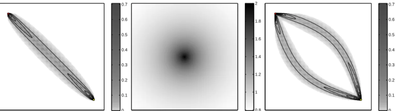
Figure 1 shows two examples of subgradient computations. Near a degenerate con-figuration, we can see that the subgradient g might be located around several minimal curves. 0 0.1 0.2 0.3 0.4 0.5 0.6 0.7 0.8 1 1.2 1.4 1.6 1.8 2 0 0.1 0.2 0.3 0.4 0.5 0.6 0.7

Figure 1: On the left, _∇ξU(x1) and some of its iso-levels for ξ = 1. In the middle, a non

constant metric ξ(x) = 1/(1.5− exp(−||c − x||)), where c is the center of the image. On the right, an element of the superdifferential of the geodesic with respect to the metric shown in the middle figure.

Anisotropic metrics. The geodesic distance and its subgradient can be defined for more complicated Riemannian metric ξ that depends both on the location γ(t) of the curve and on its local direction γ′_(t)/|γ′_{(t)|. The algorithm presented in this paper extends to this}

more general setting, thus allowing to design arbitrary anisotropic Riemannian metric. We decided however to restrict our attention to the isotropic case, that has many practical applications.

1.3 Previous Works and Contributions

Geodesic distance computation. The estimation of distance maps _Uξ _{has been}

in-tensively studied in numerical analysis and can be approximated on discrete grid of N with the Fast Marching Method of Sethian [13], and Tsitsiklis [14] in O(N log(N )) opera-tions. This algorithm has opened the door to many application in computer vision where the minimal geodesic curves extracts image features, see for instance [13, 8]. Section 2 recalls the basics of the discretization of geodesic distance and Section 2.3 details the front propagation procedure underlying the Fast Marching method.

Geodesic distance optimization. The optimization of _Uξ _{with respect to ξ is much}

less studied. It is however an important problem in some specific fields, such as for landscape design, traffic congestion and seismic imaging. In these applications, the metric ξ is optimized to meet certain criteria, or is recovered by optimization from a few geodesic distance measures.

This paper tackles directly the problem of optimizing quantities involving the distance function_Uξ _{by computing a subgradient ∇}

point x. The Subgradient Marching algorithm is described in Section 3. It follows the optimal ordering used by the Fast Marching, making the overall process only O(N2_{log(N ))}

to compute a subgradient of the maps ξ7→ Uξ_{(x) for all the grid points x.}

This Subgradient Marching computes an exact subgradient of the discrete geodesic distance, so that it can be used to minimize variational problems involving geodesic dis-tances. We believe it is important to first discretize the problem of interest and perform an exact minimization of the discrete problem. As far as geodesic quantities are involved, discretizing optimality condition of a continuous functional is indeed highly unstable. Landscape design. Shape design requires the modification of the Riemannian metric defined by the first fundamental form of the surface. Minimization of geodesic length distortion is a well studied criterion to perform surface flattening and shape comparison, see for instance [3].

This paper tackles directly the problem of optimizing a Riemannian metric ξ. The example of landscape design using a fixed amount of resources is studied in Section 4.1. The length of geodesics is maximized under local and global constraint on the metric. This problem has a unique solution that can be found using a subgradient computed with our Subgradient Marching algorithm.

An application to travel time tomography is shown in Section 4.3. A subgradient descent allows one to find a local minimum of a variational energy involving geodesic distances.

Traffic congestion. A continuous generalization of the Wardrop equilibria [15], origi-nally proposed in [5], involves the maximization of a concave functional depending on the geodesic distances between landmarks. A subgradient descent approximates this continu-ous solution and [1] describes an algorithm that makes use of our Subgradient Marching. Section 4.2 recalls basic facts of this congestion approximation and shows some numerical examples.

Seismic imaging. Seismic imaging computes an approximation of the underground from few surfaces measurements [6, 11]. This corresponds to an ill posed inverse problem that is regularized using smoothness prior information about the ground and simplifying as-sumption about wave propagation. Discarding multiple reflexions, the first arrival time of a pressure wave corresponds to the geodesic distance to the source, for a Riemannian metric ξ that reflects the properties of the underground.

The recovery of ξ from a few measurements dξ(xi, xj) between sources xi and sensors

xj corresponds to travel time tomography. A least square recovery of ξ involve the

opti-mization of the geodesic distance. It has been carried over using for instance adjoint state methods [6, 11] that involve many computations of the geodesic map _Uξ _{for a varying}

metric ξ. Our Subgradient Marching algorithm allows to find a local minimum of the regularized least square energy using a descent method.

2

Discrete Geodesic Distances

2.1 Discretization

Eikonal Equation Our approach to minimize geodesic distances first defines a discrete geodesic distance _Uξ_{, solution of a discretized partial differential equation. A discrete}

x

0

x

1

x

0

x

1

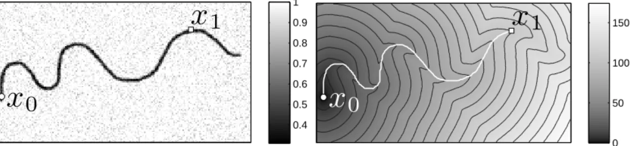
Figure 2: Example of the minimal path computation using the Fast Marching algorithm. On the left: the metric ξ. On the right: The minimal action mapU and the minimal path linking x1 to x0.

variational problems involving geodesic distances. This is a general framework that could be extended to a larger class of non-linear partial differential equations.

The geodesic map_Uξ_{(x) defined in (1.3) is the unique viscosity solution of the Eikonal}

non-linear PDE (see [10])

(

k∇Uξ_{(x)k = ξ,}

Uξ_(x 0) = 0.

(2.1) The computation ofUξ_{(x) thus requires the discretization of (2.1) so that a numerical}

scheme captures the viscosity solution of the equation.

Upwind Discretization In the following, we describe the computation in 2D and as-sume that the domain is Ω = [0, 1]2, although the scheme carries over for an arbitrary domain in any dimension.

We will also drop the dependence on ξ and x0 of the distance mapUξ=U to ease the

notations. The geodesic distance map Uξ _{is discretized on a grid of N = n× n points, so}

thatUi,j for 0≤ i, j < n is an approximation of Uξ(ih, jh) where the grid step is h = 1/n.

The metric ξ is also discretized so that ξi,j = ξ(ih, jh).

Classical finite difference schemes do not capture the viscosity solution of (2.1). Upwind derivative should be used instead

D1Ui,j := max{(Ui,j− Ui−1,j), (Ui,j− Ui+1,j), 0}/h,

D2Ui,j := max{(Ui,j− Ui,j−1), (Ui,j− Ui,j+1), 0}/h.

As proposed by Rouy and Tourin [12], the discrete geodesic distance map _{U = (U}i,j)i,j is

found as the solution of the following discrete non-linear equation that discretizes (2.1) D_{U = ξ where DU}i,j=

q

D1Ui,j2 + D2Ui,j2 . (2.2)

Rouy and Tourin [12] showed that this discrete geodesic distanceU converges to Uξ _when

h tends to 0.

Figure 2 shows an example of a discrete geodesic distance map _{U. The metric ξ has a} low value along a black curve, so that the geodesic curves tends to follow this feature. An example of geodesic curve is shown on the right, that is obtained by a numerical integration of the ordinary differential equation (1.4).

2.2 Concavity of the Geodesic Distance

To solve variational problems involving the geodesic distance dξ(x0, x), for x = (ih, jh),

one would like to differentiate with respect to ξ the discrete distance map Ui,jξ , obtained

by solving (2.2). Actually, this is not always possible, since the mapping ξ 7→ Ui,jξ is not

necessary smooth. The following proposition proves that _Ui,jξ is a concave function of ξ and this allows for superdifferentiation (the correspondent of subdifferential for concave functions instead of convex).

Proposition 2.1. For a given point (i, j), the functional ξ _{7→ Ui,j}ξ is concave. Proof. In the following we drop the dependence on (i, j) and note _Uξ _=Uξ

i,j. Thanks to

the homogeneity, it is sufficient to prove super-additivity. We want to prove the inequality Uξ1+ξ2

≥ Uξ1 +_Uξ2

.

Thanks to the comparison principle of Lemma 2.2 below, it is sufficient to prove that ξ1+

ξ2 ≥ D(Uξ1+Uξ2), where the operator D is defined in (2.2). This is easily done if we notice

that the operator D is convex (as it is a composition of the function (s, t) _7→ √s2_{+ t}2_,

which is convex and increasing in both s and t, and the operator D1 and D2, which are

convex since they are produced as a maximum of linear operators) and 1−homogeneous, and hence it is subadditive, i.e. it satisfies D(u + v)_{≤ Du + Dv.}

Lemma 2.2. If ξ ≤ η, then Uξ_{≤ U}η_.

Proof. Let us suppose at first a strict inequality ξ < η. Take a minimum point forUη_{− U}ξ

and suppose it is not the fixed point x0. Computing D and using sub-additivity we have

η = DUη _{≤ D(U}η_{− U}ξ_{) + DU}ξ _{= D(U}η _{− U}ξ_{) + ξ,}

which gives D(_Uη_−Uξ_{)≥ η−ξ > 0. Yet, at minimum points we should have D(U}η_−Uξ_{) =}

0 and this proves that the minimum is realized at x0, which impliesUη− Uξ ≥ 0.

To handle the case ξ ≤ η without a strict inequality, juste replace η by (1 + ε)η and notice that the application η_{7→ U}η _{is continuous.}

2.3 Fast Marching Propagation

The Fast Marching algorithm, introduced by Sethian in [13] and Tsitsiklis in [14], allows to solve (2.2) in O(N log(N )) operations using an optimal ordering of the grid points. This greatly reduces the numerical complexity with respect to iterative methods, because grid points are only visited once.

We recall the basic ideas underlying this algorithm, because our Subgradient Marching computation of_∇ξUξ(x) makes use of the same ordering process.

The values of U may be regarded as the arrival times of wavefronts propagating from the source point x0 with velocity 1/ξ. The central idea behind the Fast Marching method

is to visit grid points in an order consistent with the way wavefronts propagates.

In the course of the algorithm, the state of a grid point (i, j) passes successively from

Far (no estimate of_Ui,j is available) to Trial (an estimate ofUi,j is available, but it might

not be the solution of (2.1)) to Known (the value of _Ui,j is fixed and solves (2.1)). The

set of Trial points forms an interface between Known points (initially the point x0 alone)

and the Far points. The Fast Marching algorithm progressively propagates this front of