HAL Id: hal-00940830
https://hal.archives-ouvertes.fr/hal-00940830
Submitted on 11 Feb 2014
HAL is a multi-disciplinary open access
archive for the deposit and dissemination of
sci-entific research documents, whether they are
pub-lished or not. The documents may come from
teaching and research institutions in France or
abroad, or from public or private research centers.
L’archive ouverte pluridisciplinaire HAL, est
destinée au dépôt et à la diffusion de documents
scientifiques de niveau recherche, publiés ou non,
émanant des établissements d’enseignement et de
recherche français ou étrangers, des laboratoires
publics ou privés.
Probabilistic Place Recognition with Covisibility Maps
Elena Stumm, Christopher Mei, Simon Lacroix
To cite this version:
Elena Stumm, Christopher Mei, Simon Lacroix. Probabilistic Place Recognition with Covisibility
Maps. IEEE/RSJ International Conference on Intelligent Robots and Systems (IROS), Nov 2013,
Tokyo, Japan. pp.4158 - 4163. �hal-00940830�
Probabilistic Place Recognition with Covisibility Maps
Elena Stumm
1, Christopher Mei
1and Simon Lacroix
1Abstract— In order to diminish the influence of pose choice during appearance-based mapping, a more natural repre-sentation of location models is established using covisibility graphs. As the robot moves through the environment, visual landmarks are detected, and connected if seen as covisible. The introduction of a novel generative model allows relevant subgraphs of the covisibility map to be compared to a given query without needing to normalize over all previously seen locations. The use of probabilistic methods provides a unified framework to incorporate sensor error, perceptual aliasing, decision thresholds, and multiple location matches. The system is evaluated and compared with other state-of-the-art methods.
I. INTRODUCTION
The desire for long-term, autonomous navigation in un-mapped environments is becoming increasingly important for a variety of mobile robotic platforms and applications [1], [2]. In order to make this task feasible, the navigation platform must be extremely robust to errors, even in un-expected, dynamic, and possibly self-similar environments. This paper focuses on visual place recognition for mobile robots, building on the works of [3], [4] by establishing generative location models using covisibility maps.
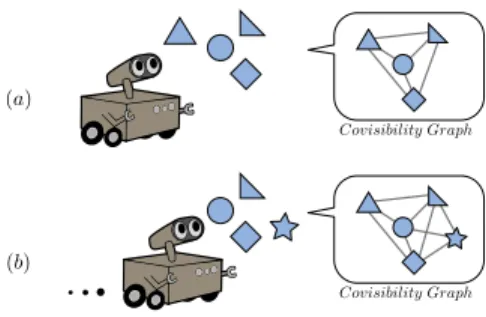
Ideas inspired from the text-document retrieval field (see [5] for an overview) are used to find previously seen locations which match a query observation. Locations are represented by a bag-of-words model, with words provided by quantized visual features and places used analogously to documents, as is common in recent literature [4], [6], [7], [8]. However, unlike typical pose-based implementations which rely on single-image location models, relevant “virtual locations” are retrieved as subgraphs from a covisibility graph at query time, therefore dubbed a dynamic bag-of-words approach [3]. This covisibility graph is constructed as the robot explores the environment, by noting which landmarks are observed together in a graph structure. The basic mapping concept is depicted in Fig. 1. By working with this covisibility graph, a more truthful, continuous rep-resentation of the environment is used, rather than a discrete selection of arbitrary poses from the robot’s trajectory. Places are now defined using direct properties of the environment (landmarks), and become less dependent on variations in trajectory while eliminating the problem of pose selection.
Once the virtual locations are retrieved, a probabilistic framework is used to identify any potential matches between the query and previously seen locations. Development of a proper generative model is a key factor for providing useful results, especially in challenging environments. In
1
CNRS; LAAS; 7 avenue du colonel Roche, F-31077 Toulouse, France ; Universit´e de Toulouse ; UPS, INSA, INP, ISAE; LAAS; F-31077 Toulouse, France ;{stumm, cmei, simon} at laas.fr
Fig. 1. As the robot moves, it makes observations, detects landmarks, and notes which ones were seen together in a graph structure. Here you can see a simple example of two steps as a robot moves forward through the environment, and the resulting covisibility graph.
the context of performing loop-closure during SLAM, an incorrect match is capable of causing large mapping errors [9], so therefore the described framework must have a very low false positive rate. In this paper, a rigorous probabilistic method allows for inherent confidence thresholds, and can handle problematic situations such as self-similar locations (perceptual aliasing) by understanding the likelihood of scene elements. The method developed here can additionally cope with erroneous maps which may contain more than one instance of the same location (for example if previous place recognition fails), due to the fact that it does not need to normalize probabilities across all previously seen locations. This method can take advantage of the covisibilty structure to asses several reprsentations of the same scene in order to find the best match and increase precision and recall characteristics.
The next section discusses the relevant background re-search, and current state-of-the-art work. Then the following two sections provide details on the covisibility framework and probabilistic approach. Finally, some test results and comparisons with previous work will be introduced.
II. RELATEDWORK
In recent years, appearance-based loop-closure and map-ping has been brought to the forefront since the introduction of visual bag-of-word techniques [6] and the popular FAB-MAP (Fast Appearance-Based Mapping) implementations [1], [4]. In these, an image is represented by a set (or bag) of quantized local image descriptors (or words) belonging to a predefined dictionary. This representation is easy to work with and fairly robust in the presence of lighting changes, view-point changes, and dynamic environments. Relevant images can be retrieved quickly using an inverted index system [6], and possibly matched to a query using word-frequency scoring techniques such as TF-IDF (Term
Frequency - Inverse Document Frequency [6]) [3], [7], [8] or probabilistic models [4], [10].
The formulation of a generative model for place recogni-tion in FAB-MAP [4] is fundamental work on the topic. This allows for a natural and intuitive way to incorporate dynamic environments and perceptual aliasing, without needing to tune extra parameters to reduce false positives. Additionally, decision thresholds for matching locations become clear probabilities. Discriminative models have also been shown to produce good results without knowledge of hidden vari-ables [10], however at the risk of unclear thresholds and heavy reliance on training data.
Inclusion of such place recognition techniques has en-abled significant improvements in long-term localization and mapping, employed in datasets up to distances of 1000 km, containing drastic lighting changes and many self-similar locations which cause perceptual aliasing [1], [2].
Impressive as these systems are, there is still room for im-provement in terms of how locations are modeled. Abstrac-tion from single image locaAbstrac-tion models has been addressed in the work of [2], [3], [11], [12]. Location models built using specific poses in the robot’s trajectory imply that the robot must visit the same arbitrary pose in order to recognize any relevant loop-closures. CAT-SLAM [2] moves towards a con-tinuous representation, but requires local metric information. In [11] and [12] comparisons are made with sequences based on time, under the assumption that the speed remains fairly consistent. The work of [3] dynamically queries location models as cliques from a covisibility graph of landmarks which are connected if seen together. These location models are then based on the underlying environmental features, rather than the discretization of the robot’s trajectory in the form of individual images, or sequences of images in time. This paper describes an appearance-based method in which dynamic virtual locations are retrieved as cliques from a covisibility graph of landmarks, and then a Bayesian framework is used to asses place recognition.
III. THECOVISIBILITYFRAMEWORK
This section outlines how the environment is represented as a graph of visual landmarks, where covisibility defines connectivity. Subsequently, the notion of virtual locations is presented, with a description of how they are retrieved from the graph at query time. These concepts originate in the work of [3], with an explanation given here for completeness. Note that one significant difference in this work is that overlapping virtual locations are now permissible, giving even further abstraction from discrete location choice. Eval-uation of overlapping virtual locations is feasible because of the probabilistic framework which will be discussed in section IV-B.
A. Creating a Covisibility Map
A covisibility map,Mt, is an undirected graph, with nodes
representing landmarks (distinct visual features), and edges representing covisibility between each landmark.
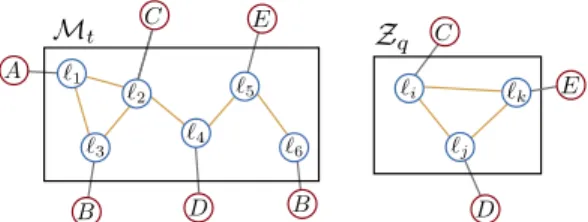
Fig. 2. The covisibility map,Mt, is shown on the left, and the current query observation, Zq on the right. The figure also depicts which word (represented as A, B, C, D or E) is associated with each landmark, ℓi.
As each image is processed, a set of visual features, ℓi,
are detected and represented by a vectorial descriptor such as SIFT [13] or SURF [14]. The landmark is furthermore associated with a quantized visual word, which is taken by the closest match in a pre-trained visual dictionary, V [6]. Thus, each image provides a set of words, which represent an observationZt, which is able to maintain some invariance to
view-point and lighting changes. Between subsequent image frames, some features are tracked, and then represented as the same landmark, ℓi. A simple example of a covisibility
map and query observation can be seen in Fig. 2.
The current map, Mt, is updated as information from
each new image is processed. The map is implemented as a sparse clique matrix, Ct, with each column representing
an observation Zt, and each row representing a particular
landmark, ℓi. Therefore the value in row r, and column c
indicates whether or not landmark ℓrwas seen in observation
Zc. An adjacency matrix, At, for the covisibililty graph can
simply be found by taking At = H(CtCtT) (with H(·)
being the element-wise unit step function), but is not needed explicitly in this work.
In addition to these matrices, an inverted index between visual words and observations is maintained, for efficient look-up during the creation of virtual locations [6].
In the simple example of Fig. 2, if at time k there are4 ob-servations (Z1 = {ℓ1, ℓ2, ℓ3}, Z2 = {ℓ2, ℓ4}, Z3 = {ℓ4, ℓ5},
andZ4= {ℓ5, ℓ6}), then the clique matrix, adjacency matrix,
and inverted index are given by:
C4= 1 0 0 0 1 1 0 0 1 0 0 0 0 1 1 0 0 0 1 1 0 0 0 1 A4= 1 1 1 0 0 0 1 1 1 1 0 0 1 1 1 0 0 0 0 1 0 1 1 0 0 0 0 1 1 1 0 0 0 0 1 1 A : {Z1} B : {Z1,Z4} C : {Z1,Z2} D : {Z2,Z3} E : {Z3,Z4}
B. Retrieving Relevant Virtual Locations
At query time, virtual locations similar to the query image need to be retrieved from the covisibility graph, in order to be compared as a potential match. The idea is to find any clusters of landmarks in the map, which may have generated the given query. Because new virtual locations are drawn from the graph for each specific query, they are more closely linked to the actual arrangement of landmarks in the environment than individual images would be. This provides a more adaptable solution to place recognition, compared to methods which rely on pose-based location models. Defining places using covisibility avoids the need for time-based image groupings which rely on prior motion knowledge [11] or more exhaustive key frame detection [15].
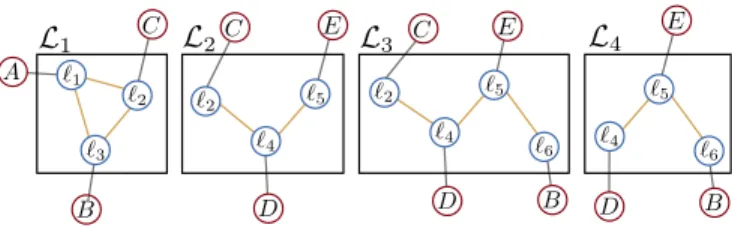
Fig. 3. Given the queryZq= {C, D, E} and covisibility map Mt(both shown in Fig. 2), will produce four virtual locations,L1,L2,L3 &L4.
The process of finding relevant virtual locations will now be described, with the aid of Figures 2 and 3, and the simple example introduced in section III-A:
• Using the inverted index, a list of observation cliques
(columns in Ct), containing words from the current
query observation, Zq, can be found. In the example,
Zq = {C, D, E}, and so the relevant observation
cliques are{Z1,Z2,Z3,Z4}.
• Then, these clusters are extended to strongly connected cliques (sharing a certain percentage of covisible land-marks). This covisibility parameter represents the proba-bility of re-observing landmarks between images. Refer to [3] for a discussion on the influence of this parameter. This will extend clique Z2 to Z3, clique Z3 to Z2 &
Z4, cliqueZ4toZ3(which all co-observe 50% of their
landmarks), and Z1 with nothing (because it doesn’t
share enough landmarks with any other cliques).
• The result is sets of landmarks/words, which in
turn, provide models for a set of virtual locations, {L1,L2, . . . ,LM}. Four virtual locations are produced
for the given example, and are shown in Fig. 3.
• Note that this set of virtual locations provides a direct match to the query, despite the fact that those landmarks were never directly covisible in any observation.
IV. THEPROBABILISTICFRAMEWORK
Once found, each virtual location needs to be evaluated, to determine if it matches the query or not. This is done by calculating the posterior probability under a Bayesian framework. Developing a probabilistic model is critical for providing system reliability. Since any incorrect matches can cause fundamental errors in the map [9], a certain level of confidence is required when making decisions about data associations. Obtaining the corresponding probabilities through a generative model provides the means to do this, while naturally incorporating aspects such as sensor error, perceptual aliasing, and dynamic environments. Rather than assuming a fixed number of independent and discrete loca-tions in the world ([1], [2], [3], [7]), the model described here allows overlapping and duplicate locations.
The posterior probability of a virtual location can be found using Bayes’ rule:
P(Li|Zq) =
P(Zq|Li)P (Li)
P(Zq)
(1)
whereLi is a particular virtual location, andZq is the query
observation given by a set visual words {z1, z2, . . . , zN}.
2 e1 |V| z2 z1 z|V| e e
Fig. 4. Graph of the observation model, with observed variables shaded in gray. A location consists of a set of visual elements en, which are then observed by an imperfect sensor, giving measurements zn.
The result can be used to infer whether a location has already been observed, thus determining if loop closure has occurred. A loop closure event can be used to gather semantic information and provide data association between visual features.
For classification tasks, only the class which maximizes the posterior is desired, meaning that normalization is not required [5]. However, in our application, a normalized probability is needed for making decisions with a high degree of certainty. In addition, there may be more than one virtual location which matches the query; for instance if a previous loop closure was missed. Thus, simply finding the maximizing argument is not enough, adding significant complexity to the problem, as calculating the normalization term is computationally expensive and requires care to ensure samples are representative.
The following sections will now outline the calculation of each probability in (1); section IV-A will cover the likelihood term, section IV-B will cover the normalization term, and section IV-C will cover the prior.
A. Calculating the Observation Likelihood, P(Zq|Li)
The query observation, Zq, is represented as a binary
word-existence-vector of length equal to the number of words in the visual dictionary,V:
hz1q, zq
2, . . . , z
q
|V|i
And the observation of a virtual location,ZL, is represented
analogously as: hzL 1, z L 2, . . . , z L |V|i
Note that the negative information (lack of a word) is explicitly considered; however frequency information (word count) is removed from the observations. Ignoring word frequencies is justified by the fact that features tend to appear in bursts, where most of the information is provided by the presence (or lack of presence) of the word, rather than the number of occurrences of the word [16].
The observation likelihood is found under a Naive-Bayes assumption, where the likelihood of each of the individual visual words, zn, are assumed to be independent given the
virtual location, Li. This reduces the term to a product of
individual word likelihoods given in (2a).
The observation model includes an existence layer for underlying scene elements, as is also done in [4] (see Fig. 4 for reference). In this case, en is introduced as a hidden
layer, which represents the true existence of scene elements generated by Li. The observations zn represent (possibly
The observation likelihood can therefore be written using the sum rule of probability as (2b), which simplifies to (2c) under the assumption that detection is independent of location: P(zn|en=α, Li) = P (zn|en=α) (see Fig. 4) [4].
P(Zq|Li) ≈ |V| Y n=1 P(znq|Li) (2a) = |V| Y n=1 X α∈{0,1} P(zq n|en=α, Li)P (en=α|Li) (2b) = |V| Y n=1 X α∈{0,1} P(zq n|en=α)P (en=α|Li) (2c)
The term P(zn|en=α) represents the sensor detection
probabilities. For example, the false negative probability of missing an element which exists, P(zn=0|en=1); and the
false positive probability of observing an element which doesn’t exist, P(zn=1|en=0), can be empirically estimated
using extracted features from representative images. Finally, the likelihood of a particular element existing in the location, P(en=α|Li), is estimated from the observation
we have of the virtual location, ZLi, the sensor model and
prior knowledge about how common the element is [17]. P(en=α|Li) = P (en=α|znL) (3a) = P(z L n|en=α)P (en=α) P(zL n) (3b) = P(z L n|en=α)P (en=α) X β∈{0,1} P(zL n|en=β)P (en=β) (3c)
Although the complexity scales with the number of words in the vocabulary, the sparse nature of observations can be used to greatly reduce computation in most cases. Note that the model could be further extended to remove the conditional independence assumption between words, for instance by using a Chow-Liu tree as done in [4]. Doing so would improve results in the presence of slight scene changes, but for simplicity has not been implemented here. See [4] for a thorough analysis of such observation models. B. Calculating the Normalization Term, P(Zq)
Calculation of the P(Zq) term is rarely done in practice,
as most applications only require maximizing the probability, meaning that normalizing the probabilities is not required. True probabilities, and therefore normalization, are necessary for dealing with perceptual aliasing, and making reliable decisions and data associations. The main difficulty in doing this lies in the fact that a model is needed for unknown locations, which we will approximate using location samples. The approach to estimating this term is to calculate P(Zq| ¯Li) (the likelihood of Zq given any other location),
and then marginalize to find P(Zq):
P(Zq) = P (Zq|Li)P (Li) + P (Zq| ¯Li)P ( ¯Li) (4)
P(Zq| ¯Li) is calculated analogously to P (Zq|Li) but using
a set of sample locations from a previously recorded dataset to estimate ¯Li.
This approach is different from that used in other place recognition frameworks such as FAB-MAP [4]. The differ-ence is that in other works, probabilities are summed over all locations in the map, plus an unknown location:
P(L1|Zq) + P (L2|Zq) + . . . + P (Lu|Zq) = 1 (5)
whereas in this work,
P(Li|Zq) + P ( ¯Li|Zq) = 1 (6)
for eachLiseparately. Equation (5) is based on an underlying
assumption that each location is only represented once, thereby assuming no loop closures will be missed, and that the map is accurate. As previously mentioned, there may in fact be more than one match to the query. This can happen when a previous loop closure is missed – leaving two or more representations of the location in the covisibility map, or if there are overlapping virtual locations such as described in section III-B. In addition, images immediately surrounding the query do not need to be removed from consideration as commonly done ([1], [7]), since these local matches will not steal probability mass from others. Another benefit of this technique is that probabilities no longer need to be normalized over all locations in the map, leaving room for efficiency improvements over other techniques. The consequences of improper normalization are illustrated at the end of section V.
C. Calculating the Location Prior, P(Li)
The location prior is estimated without the use of any motion prediction models. This is in part due to the fact that this work is meant to be kept robust to unpredictable movements and kidnapped robot situations. In practice, the effect of this prior is not especially strong, and it is therefore not a critical parameter. This is evident when comparing the order of magnitude of the observation likelihood (a product of probabilities over thousands of visual words) to that of a location prior. The weak influence of this term is also documented in [4]. Therefore most of the prior probability is assigned to unobserved locations, conservatively favoring unobserved locations (to avoid false positives). In future work, other cues could be used to more accurately estimate the location prior; such as global visual features or additional sensory information.
V. EXPERIMENTALEVALUATION
In order to evaluate the performance of the proposed framework, datasets of image streams tagged with the real position information are used to investigate precision and recall characteristics. As the image sequence progresses, the current image can be extended to its covisible range (in the same manner as virtual locations are extended) and used as a query to search for matches within the covisibility map from the same time step. This method of query expansion provides more context and suppresses false positives. It is similar to
City Centre Begbroke
Fig. 5. Example images from the Begbroke and City Centre sequences. concepts used in text and image retrieval [18], but can take advantage of covisibility to greatly simplify the expansion process. The results of other approaches (namely [3] and [4]) are used as benchmarks, and therefore evaluation is done here using datasets from these works.
The image sequence used in the work of [3] will be referred to here as the Begbroke sequence. It consists of 1 km of outdoor trajectory from a forward facing camera, with roughly 0.3 m image spacing (see Fig. 5 for example images). The sequence consists of three loops, and therefore provides many loop closures. This particular sequence is relatively difficult for loop-closure-detection, due to a mini-mal amount of distinguishing features (consisting mostly of paved paths, grass, and trees).
Urban datasets from [4], referred to as the New College and City Centre sequences, provide many challenging ex-amples of dynamic elements and perceptual aliasing. These two datasets cover approximately 2 km each, with left and right facing images provided at 1.5 m intervals (see Fig. 5 for example images).
For this evaluation, loop closures are defined to be positive if within a given radius of the query image (the spanned distance of the query images for these tests). Precision and recall are calculated by thresholding the posterior probability given by (1) and comparing the poses of cliques in the identified virtual locations with the ground truth. Any virtual location which contains cliques within the given radius of ground truth are considered as true positives.
When evaluating the Begbroke sequence, images from City Centre dataset are used to provide sample locations to the system. Similarly, during evaluation of the City Centre sequence, images from the New College dataset are used. In addition, the visual dictionary provided with the datasets from [4] is used across all systems. This indicates that collecting samples and training images that will work in a variety environments is feasible.
Tests were made using three systems: the one described in this paper (referred to here as COVISMAP), the Naive-Bayes implementation of FAB-MAP1.0 [4], and the dynamic bag of words system presented in [3]. The precision-recall results are shown in Fig. 6. In all tests, no data associations were made between landmarks as a result of loop closures, local matchings were allowed, and the same samples were provided to each system. Parameters are kept the same across different datasets, with the exception of the covisibility pa-rameter, due to the change in image spacing and orientation between the two datasets. An example of a query and a
(a) Precision-recall for the Begbroke sequence.
(b) Precision-recall for the City Centre sequence.
Fig. 6. Precision-recall results are shown for the system described in this paper (COVISMAP), Naive-Bayes FAB-MAP [4], and the dynamic bag-of-words approach with TF-IDF scoring [3].
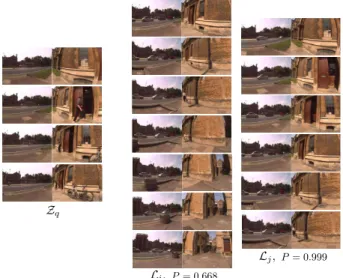
Fig. 7. Examples of a query and a few resulting virtual locations from the City Centre sequence, with posterior probabilities listed below.
couple of the resulting virtual locations from the City Centre dataset are shown in Fig. 7, with the corresponding match probabilities given by the framework of this paper shown below.
To clarify, the performance presented here for FAB-MAP on the City Centre dataset is different than that of the original publication [4] for several reasons. Firstly, the images used for sample locations are different, in order to keep a consistent comparison between systems. Secondly, the ground truth is determined by a radius from the query image, rather than hand-labeled; often including images which are close by, but not a visual match. Finally, in [4], the prior probability of images immediately preceding the query image
image from first loop image from second loop
image from third loop: (previous position) image from third loop:
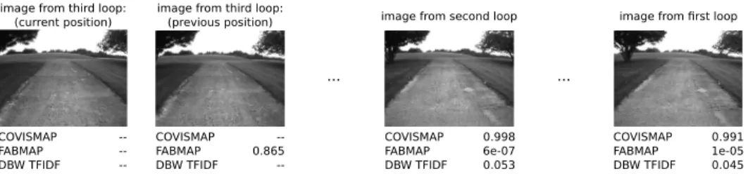
(current position) COVISMAP FABMAP DBW TFIDF 0.991 1e-05 0.045 COVISMAP FABMAP DBW TFIDF 0.998 6e-07 0.053 COVISMAP FABMAP DBW TFIDF --0.865 --COVISMAP FABMAP DBW TFIDF --... ...
Fig. 8. Example of a location from the Begbroke sequence which is passed several times, and the matching scores resulting from a query generated during the third pass. Scores are shown for the system described in this paper (COVISMAP), Naive-Bayes FAB-MAP [4], and the dynamic bag-of-words approach with TF-IDF scoring [3]. Images which are part of the query are not given scores and indicated with dashes - - (including those added by query expansion). Therefore only the FAB-MAP system provides a score for the image next the query position here, since each image represents a distinct location. were artificially set to zero to eliminate competition between
local and further matches, but this was not done here. Fig. 8 compares matching scores for a repeatedly ob-served location for the different algorithms. The benefit of probabilistic methods are especially clear when looking at the thresholds used to determine matches; Fig. 8 shows that the COVISMAP and FAB-MAP formulations provide meaningful scores representing probabilities in the range [0, 1], whereas the TF-IDF approach provides scores which require unintuitive and possibly varying thresholds. Fur-ther advantages are also evident from Fig. 8, where FAB-MAP fails to give high scores when the same location is passed several times. This is due to the fact that FAB-MAP probabilities must be normalized across all locations, meaning that the probability mass can be split across several representations of the same location in the map.
VI. CONCLUSION
This article has proposed a framework for appearance-based place recognition and loop closure. It uses a represen-tation that builds a map using the covisibility of landmarks, in order to reduce the influence of pose choice when modeling locations. A dynamic bag-of-words scheme provides relevant virtual locations to the query. The virtual locations pro-vide representations of places, which can comprise multiple images containing covisible elements, and may overlap, allowing for a more continuous progression of locations. Once retrieved, these virtual locations are evaluated using Bayesian reasoning to asses which places may have already been seen before. The system can model perceptual aliasing, sensor error, and also redundant locations in the map due to the derived normalization methods, thus providing the means for increased reliability.
Testing of the framework has been done, in order to evaluate performance and compare with other methods. The results compare well with the state-of-the-art, but more work needs to be done with a variety of datasets to confirm reliability and provide a more thorough assessment.
Potential future work includes extending the probabilistic model to remove assumptions such as the Naive-Bayes ap-proximation, and incorporating other sources of information into the model such as global image attributes. Another interesting continuation is to investigate further uses of the covisibility graph, such as learning how to use structural in-formation in the graph to infer types of places and correlation between places in the map.
REFERENCES
[1] M. Cummins and P. Newman, “Appearance-only SLAM at large scale with FAB-MAP 2.0,” The Int. Journal of Robotics Research, Aug. 2011.
[2] W. Maddern, M. Milford, and G. Wyeth, “CAT-SLAM: probabilistic localisation and mapping using a continuous appearance-based trajec-tory,” The Int. Journal of Robotics Research, Apr. 2012.
[3] C. Mei, G. Sibley, and P. Newman, “Closing loops without places,” in IEEE Int. Conf. on Intelligent Robots and Systems, Taipai, Taiwan, 2010.
[4] M. Cummins and P. Newman, “FAB-MAP: Probabilistic localization and maping in the space of appearance,” The Int. Journal of Robotics Research, Jun. 2008.
[5] C. D. Manning, P. Raghavan, and H. Sch¨utze, Introduction to Informa-tion Retrieval. New York, USA: Cambridge University Press, 2008. [6] J. Sivic and A. Zisserman, “Video google: A text retrieval approach to object matching in videos,” IEEE Int. Conf. on Computer Vision, 2003.
[7] A. Angeli, D. Filliat, S. Docieux, and J.-A. Meyer, “A fast and incremental method for loop-closure detection using bags of visual words,” IEEE Trans. on Robotics, Special Issue on Visual SLAM, Oct. 2008.
[8] T. Botterill, S. Mills, and R. Green, “Bag-of-words-driven, single-camera simultaneous localization and mapping,” Journal of Field Robotics, Mar./Apr. 2011.
[9] T. Bailey and H. Durrant-Whyte, “Simultaneous localization and mapping (SLAM): part II,” Robotics Automation Magazine, IEEE, vol. 13, no. 3, pp. 108–117, Sept. 2006.
[10] C. Cadena, D. G´alvez-L´opez, J. D. Tard´os, and J. Neira, “Robust place recognition with stereo sequences,” IEEE Trans. on Robotics, Aug. 2012.
[11] D. G´alvez-L´opez and J. D. Tard´os, “Bags of binary words for fast place recognition in image sequences,” IEEE Trans. on Robotics, vol. 28, no. 5, pp. 1188–1197, Oct. 2012.
[12] M. J. Milford and G. F. Wyeth, “SeqSLAM: Visual route-based navigation for sunny summer days and stormy winter nights,” in IEEE Int. Conf. on Robotics and Automation, St. Paul, USA, 2012. [13] D. G. Lowe, “Object recognition from local scale-invariant features,”
IEEE Int. Conf. on Computer Vision, 1999.
[14] H. Bay, A. Ess, T. Tuytelaars, and L. Van Gool, “SURF: Speeded Up Robust Features,” Computer Vision and Image Understanding, 2008. [15] A. Ranganathan and F. Dellaert, “Bayesian surprise and landmark
detection,” in IEEE Int. Conf. on Robotics and Automation, Kobe, Japan, 2009.
[16] K.-M. Schneider, “On word frequency information and negative ev-idence in naive Bayes text classification,” in Advances in Natural Language Processing. Springer, 2004.
[17] A. Glover, W. Maddern, M. Warren, S. Reid, M. Milford, and G. Wyeth, “OpenFABMAP: An open source toolbox for appearance-based loop closure detection,” in IEEE Int. Conf. on Robotics and Automation, St. Paul, USA, 2012.
[18] O. Chum, J. Philbin, J. Svic, M. Isard, and A. Zisserman, “Total recall: Automatic query expansion with a generative feature model for object retrieval,” in IEEE Int. Conf. on Computer Vision, Rio de Janeiro, Brazil, 2007.