HAL Id: hal-02989943
https://hal.archives-ouvertes.fr/hal-02989943
Submitted on 5 Nov 2020
HAL is a multi-disciplinary open access
archive for the deposit and dissemination of
sci-entific research documents, whether they are
pub-lished or not. The documents may come from
teaching and research institutions in France or
abroad, or from public or private research centers.
L’archive ouverte pluridisciplinaire HAL, est
destinée au dépôt et à la diffusion de documents
scientifiques de niveau recherche, publiés ou non,
émanant des établissements d’enseignement et de
recherche français ou étrangers, des laboratoires
publics ou privés.
Synthetic nebular emission from massive galaxies II:
ultraviolet-line diagnostics of dominant ionizing sources
Michaela Hirschmann, Stéphane Charlot, Anna Feltre, Thorsten Naab, Rachel
Somerville, Ena Choi
To cite this version:
Michaela Hirschmann, Stéphane Charlot, Anna Feltre, Thorsten Naab, Rachel Somerville, et al..
Synthetic nebular emission from massive galaxies II: ultraviolet-line diagnostics of dominant ionizing
sources. Monthly Notices of the Royal Astronomical Society, Oxford University Press (OUP): Policy
P - Oxford Open Option A, 2002, 000, pp.1 - 22. �10.1093/mnras/stz1256�. �hal-02989943�
arXiv:1811.07909v1 [astro-ph.GA] 19 Nov 2018
Synthetic nebular emission from massive galaxies II:
ultraviolet-line diagnostics of dominant ionizing sources
Michaela Hirschmann
1,2⋆, St´
ephane Charlot
1, Anna Feltre
1,3, Thorsten Naab
4,
Rachel S. Somerville
5,6, Ena Choi
7,
1Sorbonne Universit´es, UPMC-CNRS, UMR7095, Institut d’ Astrophysique de Paris, F-75014 Paris, France 2University of Vienna, Institute for Astronomy, T¨urkenschanzstrasse 17, 1180 Vienna, Austria
3Univ. Lyon, Univ. Lyon1, ENS de Lyon, CNRS, Centre de Recherche Astrophysique de Lyon, UMR5574, 69230 Saint-Genis-Laval, France 4Max-Planck-Institute for Astrophysics, Karl-Schwarzschild-Strasse 1, 85741 Garching, Germany
5Department of Physics and Astronomy, Rutgers, The State University of New Jersey, NJ 08854, USA 6Center for Computational Astrophysics, Flatiron Institute, 162 5th Ave, New York, NY 10010, USA 7Department of Astronomy, Columbia University, New York, NY 10027, USA
Accepted ???. Received ??? in original form ???
ABSTRACT
We compute synthetic optical and ultraviolet (UV) emission-line properties of galaxies in a full cosmological framework by coupling, in post-processing, new-generation nebular-emission models with high-resolution, cosmological zoom-in simu-lations of massive galaxies. Our self-consistent modelling accounts for nebular emis-sion from young stars and accreting black holes (BHs). We investigate which optical-and UV-line diagnostic diagrams can best help to discern between the main ionizing sources, as traced by the ratio of BH accretion to star formation rates in model galax-ies, over a wide range of redshifts. At low redshift, simulated star-forming galaxgalax-ies, galaxies dominated by active galactic nuclei and composite galaxies are appropriately differentiated by standard selection criteria in the classical [O iii]λ5007/Hβ versus [N ii]λ6584/Hα diagram. At redshifts z & 1, however, this optical diagram fails to discriminate between active and inactive galaxies at metallicities below 0.5Z⊙. To
robustly classify the ionizing radiation of such metal-poor galaxies, which dominate in the early Universe, we confirm 3 previous, and propose 11 novel diagnostic dia-grams based on equivalent widths and luminosity ratios of UV emission lines, such as EW(O iii] λ1663) versus O iii] λ1663/He ii λ1640, C iii] λ1908/He ii λ1640 versus O iii] λ1663/He ii λ1640, and C iv λ1550/C iii] λ1908 versus C iii] λ1908/C ii] λ2326. We formulate associated UV selection criteria and discuss some caveats of our re-sults (e.g., uncertainties in the modelling of the He ii λ1640 line). These UV diagnostic diagrams are potentially important for the interpretation of high-quality spectra of very distant galaxies to be gathered by next-generation telescopes, such as the James Webb Space Telescope.
Key words: galaxies: abundances; galaxies: formation; galaxies: evolution; galaxies: general; methods: numerical
1 INTRODUCTION
The emission from interstellar gas contains important information about the nature of ionizing sources in a galaxy. In particular, optical nebular emission lines are traditionally used to estimate whether ionization is dom-inated by young massive stars (tracing the star
for-⋆ E-mail: [email protected]
mation rate, hereafter SFR), an active galactic nucleus (hereafter AGN) or evolved, post-asymptotic giant branch
(hereafter post-AGB) stars (e.g., Izotov & Thuan 1999;
Kobulnicky et al. 1999;Kauffmann et al. 2003;Nagao et al. 2006;Kewley & Ellison 2008;Morisset et al. 2016). In fact, the intensity ratios of strong emission lines, such as Hβ, [O iii]λ5007, Hα and [N ii]λ6584, exhibit well-defined correlations, characteristic of different ionizing sources. One of the most widely used line-ratio diagnostic
dia-grams, originally defined byBaldwin et al.(1981, hereafter
BPT) andVeilleux & Osterbrock(1987) in that defined by
the [O iii]λ5007/Hβ and [N ii]λ6584/Hα (hereafter simply [O iii]/Hβ and [N ii]/Hα) ratios. This diagram has proven useful to identify the nature of the ionizing radiation in large
samples of galaxies in the local Universe (e.g.Kewley et al.
2001;Kauffmann et al. 2003), but its applicability at high redshift is still unclear. Based on a sample of about 50 star-forming galaxies and 10 confirmed AGN at z ∼ 2.3,
Coil et al.(2015) find that the local AGN/star-forming (SF) galaxy classification in the [O iii]/Hβ–[N ii]/Hα diagram robustly separates these populations in the distant Uni-verse. However, the apparent evolution of the [O iii]/Hβ ratio over cosmic time identified in several observational
studies challenges this conclusion (e.g.,Shapley et al. 2005;
Lehnert et al. 2009; Yabe et al. 2012; Steidel et al. 2014;
Shapley et al. 2015;Strom et al. 2017). In addition, at the very low metallicities expected in the youngest galaxies at
high redshifts (e.g., Maiolino et al. 2008), emission-line
ra-tios for SF- and AGN-dominated models tend to occupy
sim-ilar regions of the [O iii]/Hβ–[N ii]/Hα diagram (Feltre et al.
2016). Thus, even if optical emission lines will be
measur-able out to redshifts of several using the future James Webb
Space Telescope (JWST), their usefulness to constrain the
nature of ionizing sources in the early universe is uncertain. In recent years, interest has grown in ultraviolet (UV) nebular emission lines, such as C iii] λ1908, C iv λ1550 and He ii λ1640 lines, which can be routinely detected in star-forming galaxies at low redshift with the Hubble Space
Tele-scope and at higher redshift with near-infrared
spectro-graphs (e.g., Pettini & Pagel 2004; Hainline et al. 2009;
Steidel et al. 2014; Shapley et al. 2015; Erb et al. 2010;
Hainline et al. 2011; Stark et al. 2014, 2015; Berg et al. 2016; Vanzella 2016; Senchyna et al. 2017; Talia 2017;
Laporte et al. 2017). UV emission lines tend to be partic-ularly prominent in metal-poor, actively star-forming dwarf
galaxies at all redshifts (e.g., Stark et al. 2014;Berg et al.
2016; Senchyna et al. 2017). This is because metal-poor gas cools less efficiently than metal-rich gas, leading to higher electron temperatures and stronger collisionally ex-cited emission lines, while metal-poor stars are also hot-ter and have harder ionizing spectra than metal-rich ones
(e.g., Schaller et al. 1992; Schaerer 2003). This makes UV
emission lines attractive tracers of the ionizing radiation in metal-poor galaxies, which will be observable with JWST at redshifts way into the reionization epoch, between z ∼ 15 (Planck Collaboration 2016) and z ∼ 6 (e.g. Fan et al.
2006). Yet, to date, the dependence of these lines on the
nature of the ionizing radiation in galaxies has been far less studied than that of optical lines, and never in a cosmolog-ical context.
In a pioneering study, Feltre et al. (2016) explored
the UV emission-line properties of photoionization mod-els of SF- and AGN-dominated galaxies and proposed new line-ratio diagnostic diagrams to discriminate between the two populations, such as C iii] λ1908/He ii λ1640 ver-sus C iv λ1550/He ii λ1640 diagram. This approach (see also
Nakajima et al. 2018) relies on a blind exploration of the wide parameter space of photoionization models (ionization parameter, element abundances, depletion of metals on to dust grains, stellar and AGN properties, etc.). While highly instructive, it also presents some drawbacks: the results may
be affected by parameter combinations not found in nature; the combined effects of star formation and nuclear activity
in a ‘composite’ galaxy were not explored;1 and the
con-clusions drawn about line-ratio diagnostic diagrams do not incorporate the potential evolution of galaxy properties with cosmic time.
In this context, modelling nebular emission from galax-ies in a full cosmological framework could provide valu-able insight into the connection between observed emis-sion lines and the underlying ionizing-source properties as a function of cosmic time. Yet, fully self-consistent mod-els of this kind are currently limited by the performance of cosmological radiation-hydrodynamic simulations and in-sufficient spatial resolution on scales of individual ionized regions around stars and AGN. As an alternative, some studies proposed the post-processing of cosmological hydro-dynamic simulations and semi-analytic models with pho-toionization models to compute nebular emission of
galax-ies in a cosmological context (Kewley et al. 2013;Orsi et al.
2014;Shimizu et al. 2016;Hirschmann et al. 2017). For ex-ample, by combining chemical enrichment histories from cos-mological simulations with photoionization models of SF
galaxies, Kewley et al. (2013) proposed modified,
redshift-evolvingcriteria in the [O iii]/Hβ–[N ii]/Hα diagram to
se-lect SF galaxies while accounting for the predicted cosmic evolution of [O iii]λ5007/Hβ. Despite this progress, no study so far has either considered a full differentiation between SF, composite and AGN-dominated galaxies, or investigated the potential usefulness of UV emission lines for the classifica-tion of ionizing sources over cosmic time.
In this paper, we close this gap by appealing to the
methodology introduced by Hirschmann et al. (2017) to
model in a self-consistent way the emission from differ-ent gas compondiffer-ents ionized by differdiffer-ent sources in sim-ulated galaxies. This is achieved by coupling
photoion-ization models for AGN (Feltre et al. 2016), young stars
(Gutkin et al. 2016) and post-AGB stars (Hirschmann et al.
2017) with cosmological hydrodynamic simulations. The
re-sulting models reproduce observations of galaxies in vari-ous optical BPT diagrams involving the Hβ, [O iii]λ5007, [O i]λ6300, Hα, [N ii]λ6584 and [S ii]λλ6717, 6731 (hereafter simply [S ii]λ6724) lines, at both low and high redshifts, and accounting for the observed evolutionary trend in [O iii]/Hβ (Hirschmann et al. 2017). Our methodology, which by de-sign captures SF, composite and AGN-dominated galaxies in a full cosmological framework, provides a unique means of answering key questions we wish to address in the present study:
• To what extent are optical selection criteria, tradition-ally used to identify the nature of ionizing sources in low-redshift galaxies, still useful for classifications at high red-shift?
• Can we identify novel diagnostic diagrams in the rest-frame UV and derive corresponding selection criteria to identify the main ionizing sources of galaxies, in particular in the distant Universe?
1 Note thatNakajima et al.(2018) consider composite-like
galax-ies, by simply adopting different fractional AGN contributions, but they do not derive any selection criteria for composites.
Answers to these questions will allow proper interpretation of the high-quality spectra of very distant galaxies to be gathered by next-generation telescopes, such as JWST, pro-viding valuable insight into, for example, the relative contri-butions by star formation and nuclear activity to reioniza-tion of the Universe.
The paper is structured as follows. In Section 2, we
present the general theoretical framework of our study, in-cluding the zoom-in simulations of massive galaxies, the nebular-emission models and the way in which we combine
the former with the latter. Sections 3 and 4 describe our
main results about tracing the nature of ionizing sources in distant galaxies via standard optical and novel UV line-ratio diagnostics. We address possible caveats of our approach and discuss our findings in the context of previous
theoret-ical studies in Section 5. Finally, Section6summarizes our
results.
2 THEORETICAL FRAMEWORK
2.1 Cosmological zoom-in simulations of massive
haloes
To achieve the analysis presented in this paper, we appeal to a set of 20 high-resolution, cosmological zoom-in
simula-tions of massive haloes described in Choi et al.(2017) and
Hirschmann et al.(2017). We briefly summarise these mod-els below and refer the reader to the original studies for more details.
2.1.1 The simulation code ‘SPHGal’
The simulations used in this study were produced with a modified version of the highly parallel, smoothed particle
hy-drodynamics (SPH) code Gadget3 (Springel et al. 2005),
SPHGal. As described inHu et al.(2014), this code includes
‘modern’ numerical SPH schemes, which pass all standard tests previously reported to be problematic, such as
fluid-mixing problems (see also, Choi et al. 2017; N´u˜nez et al.
2017).
SPHGal follows baryonic processes, such as star for-mation, chemical enrichment, metal-line cooling, stellar and AGN feedback and ultraviolet photo-ionization background (Haardt & Madau 2001). Specifically, star formation and
chemical evolution are modelled as described inAumer et al.
(2013) andN´u˜nez et al.(2017). To model star formation, we
assume a temperature-dependent density threshold, above which gas particles get Jeans unstable and are stochasti-cally converted into star particles. Chemical enrichment is accounted for via type-Ia and type-II supernovae (SNe) and AGB stars, tracing 11 elements (H, He, C, N, O, Ne, Mg, Si, S, Ca and Fe) in both gas and star particles. We also
account for metal diffusion in the ISM as in Aumer et al.
(2013).
Star formation is regulated by both stellar and AGN
feedback. We adopt the approach outlined in N´u˜nez et al.
(2017) to model mass, energy and momentum injection due
to early stellar and SN feedback from different evolution-ary stages of massive stars. AGN feedback is tied to the
prescription for BH growth described inChoi et al.(2017),
where BHs accrete gas following a statistical Bondi-Hoyle
approach (Bondi 1952;Choi et al. 2012). To compute AGN
feedback from BH accretion, we do not make the widely used assumption of considering only thermal energy
re-lease into the ambient medium (e.g.,Hirschmann et al. 2014;
Naab & Ostriker 2016; Somerville & Dav´e 2015). Instead, we rely on a more physically motivated approach including both mechanical feedback, motivated by broad-absorption-line winds from quasars, and radiative X-ray feedback, due to Compton and photoionization heating and radiation
pres-sure (Ostriker et al. 2010; Choi et al. 2017). We note that
our 20 zoom-in simulations do not include any metallicity-dependent heating prescription. This is justified by the fact
that, as shown by Choi et al.(2017), such refinements are
not found to have any significant impact on basic proper-ties of massive galaxies. Adopting these sub-grid models, in particular the improved prescription for AGN feedback, we obtain fairly realistic massive galaxies, e.g. in terms of star formation histories, baryon conversion efficiencies, sizes, gas fractions, gas and stellar metallicities, hot-gas X-ray
lumi-nosities and optical emission line ratios (Choi et al. 2017;
Hirschmann et al. 2017;Brennan et al. 2018).
2.1.2 The simulation set-up
Our set of 20 cosmological zoom-in simulations is based on
a sub-set of initial conditions fromOser et al.(2010,2012)
and Hirschmann et al. (2012, 2013), adopting a WMAP3
cosmology (σ8= 0.77, Ωm= 0.26, ΩΛ= 0.74 and h = 0.72;
see, e.g.,Spergel et al. 2003). The dark-matter (DM) haloes
chosen for zoom-in re-simulations, with z = 0 virial masses
between 2.2 × 10¹²M
⊙ h−1 and 2.2 × 10¹³M⊙ h−1, were
selected from a DM-only N-body simulation with a
co-moving periodic box length L = 72 Mpc h−1and 5123
parti-cles (Moster et al. 2010). To construct the initial conditions
for the high-resolution re-simulations, individual haloes are traced back in time, and all particles closer to the halo centre than twice the radius where the mean density drops below 200 times the critical density of the universe at any given snapshot are identified. These DM particles are replaced
with particles at higher resolution with masses of mdm =
2.5 × 10⁷M
⊙h−1 for DM, and mgas = 4.2 × 10⁶M⊙h−1 for
gas, equal to that of star particles. The co-moving
gravita-tional softening length of the DM particles is 890 h−1pc, and
that of the gas and star particles 400 h−1pc.
To investigate the redshift evolution of different galaxy properties (including emission-line ratios), we construct stel-lar merger trees for the sample of 20 model galaxies
de-scribed in the previous subsection. As inOser et al.(2012),
we start by using a friends-of-friends algorithm to identify, at any simulation snapshot, a central galaxy – the host (i.e., the most massive galaxy sitting at the minimum of the halo potential well) – and its surrounding satellite (less massive) galaxies. We require a minimum of 20 stellar particles (i.e.,
a minimum mass of about 1.2 × 10⁸M
⊙) to identify a galaxy.
At z = 2, all galaxies in our sample are more massive than
about 1010M
⊙, implying that, at z < 2, we resolve mergers
down to a mass ratio of at least 1 : 100. In the analysis pre-sented in the remainder of this paper, we trace back at every time step only the most massive progenitor of a present-day galaxy, i.e., we focus on central galaxies.
Note that our limited sample of zoom-in simulations does not allow for a statistical representation of galaxies
(e.g., probability distribution), and moreover, our simulation suite probes only a subset of the parameter space (e.g., both lower-mass and higher-mass halos are missing). Neverthe-less, we emphasise that despite using a non-cosmologically representative sample for this study, our simulations do fol-low the scaling relations between various physical parame-ters (e.g. mass-metallicity relation).
2.2 Modeling of nebular emission
As in Hirschmann et al. (2017), we post-process the
re-simulations of 20 galaxies presented in Section2.1to include
nebular emission. To achieve this, we adopt the recent
pre-scriptions of Gutkin et al. (2016), Feltre et al. (2016) and
Hirschmann et al. (2017), with some minor modifications, to compute the nebular emission arising from young mas-sive stars, narrow-line regions of AGN and post-AGB stars,
as described in Section2.2.1below. All emission-line models
presented in this paper were computed using version c13.03
of the photoionization code Cloudy (Ferland et al. 2013).
Then, we couple these extensive calculations of nebular-emission models with the simulations of massive galaxies,
as described in Section2.2.2. For further details about the
nebular-emission models and coupling methodology, we
re-fer the reader to Gutkin et al. (2016), Feltre et al. (2016)
andHirschmann et al.(2017).
2.2.1 Nebular-emission models
To model Hii regions around young stars, we adopt the updated grid of nebular-emission models of star-forming galaxies computed by J. Gutkin (private communication).
As in Gutkin et al. (2016), these calculations combine the
latest version of theBruzual & Charlot (2003) stellar
pop-ulation synthesis model (Charlot & Bruzual, in prepa-ration) with Cloudy, following the method outlined by
Charlot & Longhetti(2001). The models used here include newly updated spectra of Wolf-Rayet stars from the Pots-dam Wolf-Rayet Models (PoWR; private communication from H. Todt). The resulting grid encompasses models in wide ranges of interstellar (i.e. gas+dust-phase)
metallic-ity, Z⋆, ionization parameter, U⋆, dust-to-metal mass
ra-tio, ξd, Hii-region density, nH,⋆and carbon-to-oxygen
abun-dance ratio, (C/O)⋆(see table 1 of Hirschmann et al. 2017
for a summary of all parameters). We adopt here the default
emission-line predictions ofGutkin et al.(2016) for 10
Myr-old stellar populations with constant SFR and a standard
Chabrier(2003) initial mass function (IMF; consistent with the IMF adopted in the simulations), truncated at 0.1 and
300 M⊙.2
For narrow-line regions of AGN, we adopt an updated
grid of nebular-emission models ofFeltre et al.(2016). The
new grid includes microturbulent clouds (with a microtur-bulence velocity of 100 km/s) and adopts a smaller inner radius (90 pc compared to the old radius of 300 pc for an
2 We adopt here an IMF truncated at m
up = 300M⊙, rather
than the standard 100 M⊙, to increase the strength of the
He ii λ1640 line and bring it in better agreement with observations (Senchyna et al. 2017). See also section5.2for further discussion.
AGN luminosity of 1045 erg/s) for the gas in the NLR.3 In
this prescription, the spectrum of an AGN is approximated by a broken power law of adjustable index α in the frequency
range of ionizing photons (equation 5 ofFeltre et al. 2016).
The grid of AGN nebular-emission models is parametrized in terms of the interstellar metallicity in the narrow-line
re-gion, Z•, the ionization parameter of this gas, U•, the
dust-to-metal mass ratio, ξd, the density of gas clouds, nH,•, and
the carbon-to-oxygen abundance ratio, (C/O)• (see table 1
inHirschmann et al. 2017).
To describe nebular emission from quiescent, passively evolving galaxies, we adopt the grid of ‘PAGB’ models
intro-duced inHirschmann et al.(2017), constructed by inserting
spectra of single-age, evolved stellar populations into the photoionization code Cloudy. The grid includes models in
wide ranges of stellar population age and metallicity, Z⋄,stars,
gas ionization parameter, U⋄, dust-to-metal mass ratio, ξd,
hydrogen density, nH,⋄ and interstellar metallicity, Z⋄ (see
table 1 ofHirschmann et al.(2017)).
2.2.2 Coupling nebular-emission models with zoom-in
simulations
We couple the extensive grid of nebular-emission models
described in Section 2.2.1 with the simulations of massive
galaxies described in Section2.1by selecting a SF, AGN and
PAGB emission-line model for each simulated galaxy at each redshift step. The sum of these three components makes up the integrated nebular emission of a model galaxy. In prac-tice, we select the SF/AGN/PAGB models appropriate for each galaxy by self-consistently matching all model parame-ters possibly available from the simulations (e.g., metallicity of the star-forming gas).
A few model parameters cannot be retrieved from the simulation, such as the slope of the ionizing AGN spectrum
α, the dust-to-metal mass ratio ξd, and the hydrogen gas
density in individual ionized regions nH. By considering
dif-ferent values for these parameters, their potential impact on the nebular emission of galaxies is automatically accounted for in our analysis. Specifically, we sample two values of the
dust-to-metal mass ratio, ξd= 0.3 and ξd= 0.5, in the SF,
AGN and PAGB models, as these values are closest to that of
ξd,⊙= 0.36 in the Solar neighbourhood (Gutkin et al. 2016).
We further consider two values of the hydrogen gas density
in HII-regions, nH,⋆ = 102cm−3 and nH,⋆ = 103cm−3, in
the SF models. In the AGN models, we allow for two values
of the gas density in narrow-line regions, nH,• = 103cm−3
and nH,• = 104cm−3, and two values for the UV-slope of
the AGN ionizing spectrum, α = −1.4 and α = −2.0.4 For
the PAGB models, nH,⋄= 10 cm−3 is adopted. In the next
paragraphs, we briefly describe the methodology to couple the SF, AGN and PAGB nebular models with our zoom-in galaxy simulations.
To match the SF models with simulated galaxies, we
3 Note that these modifications have been found to result in a
better agreement with the observations of NV emission lines of AGN (Mignolie, Feltre et al. in prep.).
4 In other words, we consider all permutations of the
non-constrained parameters to have the maximum possible area spanned by line ratios of a galaxy in the BPT/UV diagnostic diagrams.
associate the SF emission-line model from theGutkin et al.
(2016) grid with the gas and star parameters closest to that
of each galaxy at each simulation time step. Specifically,
we select the grid metallicity Z⋆, carbon-to-oxygen ratio
(C/O)⋆and ionization parameter log U⋆closest to the
sim-ulated global (i.e. galaxy-wide) metallicity Zgas,glob,
abun-dance ratio (C/O)gas,glob of the warm-gas phase and the
simulated ionization parameter log Usim,⋆. This uniquely
de-fines the Gutkin et al. (2016) model associated with each
simulated galaxy at each time step. Note that we com-pute the ionization parameter of a simulated galaxy
us-ing equation 1 ofHirschmann et al.(2017). As explained in
Hirschmann et al.(2017), in our approach, Usim,⋆ depends
on the simulated SFR (via the rate of ionizing photons) and
global average gas density, ρgas,glob(via the filling factor).
To associate AGN models from theFeltre et al.(2016)
grid with the nuclear activity of simulated galaxies at any simulation time step, we adopt a procedure similar to that for SF models. We take the ISM conditions for the AGN model to be the central (rather than global) ones of the simulated galaxy, i.e, in a co-moving sphere of 1-kpc ra-dius around the black hole. This size should be roughly appropriate to probe the narrow-line regions around AGN with luminosities in the range found in our simulations (see
fig. 3 ofHainline et al. 2014 and the model AGN
luminosi-ties in Fig. 6 of Hirschmann et al. 2017). We compute the
central warm-gas metallicity, Zgas,1kpc, central
carbon-to-oxygen ratio, (C/O)gas,1kpc, and central ionization
param-eter, Usim,•, derived from the central volume-averaged gas
density, ρgas,1kpc, and the bolometric AGN luminosity, LAGN
(see Hirschmann et al. 2017 for details). Then, we select the Feltre et al. (2016) model with closest Z•, log U• and
(C/O)•.
To pick a PAGB emission-line model from the
Hirschmann et al.(2017) grid for each galaxy at each simu-lation time step, we compute the average age and metallic-ity of all star particles older than 3 Gyr, and we adopt the
same global interstellar metallicity Zgas,glob, abundance
ra-tio (C/O)gas,glob and volume-averaged gas density ρgas,glob
(used to compute the ionization parameter of the gas
ion-ized by post-AGB stars Usim,⋄) as for Hii regions. We then
select the PAGB model with closest grid values of Z⋄,stars,
Age⋄,stars, Z⋄, (C/O)⋄, and log U⋄.
2.2.3 Total emission-line luminosities and line ratios of
simulated galaxies
The procedure described in the previous paragraphs al-lows us to compute the contributions of young stars, AGN and post-AGB stars to the luminosities of
vari-ous emission lines (such as LHα, LHβ, LOIII, etc.) in
a simulated galaxy. The total emission-line luminosities of the galaxy can then be calculated by summing over these three contributions. For line luminosity ratios, we
adopt for simplicity the notation LOIII/LHβ = [O iii]/Hβ.
In this study, we focus on exploring line ratios built from six optical lines, Hβ, [O iii]λ5007, [O i]λ6300, Hα,
[N ii]λ6584 and [S ii]λ6724 (as defined in Section 1), and
11 UV lines, N v λ1240 (multiplet), [N iv]λ1483+N iv]λ1487 (hereafter simply N iv] λ1485), C iv λλ1548, 1551 (here-after simply C iv λ1550), He ii λ1640, O iii]λλ1661, 1666 (hereafter simply O iii] λ1663), N iii] λ1750 (multiplet),
Si ii] λ1814 (multiplet), [Si iii]λ1883+Si iii]λ1892 (hereafter simply Si iii] λ1888), [C iii]λ1907+C iii]λ1909 (hereafter sim-ply C iii] λ1908), C ii] λ2326 and [O ii]λλ3726, 3729 (here-after simply [O ii] λ3727).
2.2.4 Total equivalent widths of nebular emission lines of
simulated galaxies
In addition to line luminosities and line ratios, we also compute the total equivalent widths (EW) of some nebu-lar emission lines. We obtain the EW of an emission line by dividing the total line luminosity by the total contin-uum flux C at the line wavelength, e.g. EW(C iii] λ1908)
= LCIII/CCIII (expressed in ˚A). The total continuum C is
the sum of the contributions by the stellar (SF and PAGB) and AGN components. For the stellar components, we ac-count for both attenuated stellar radiation and nebular re-combination continuum. For the AGN component, we con-sider only the nebular recombination continuum, and do not account for any attenuated radiation from the accreting BH. This assumption should be reasonable for type-2 AGN, where direct AGN radiation is obscured by the surround-ing torus, and only emission from the narrow-line region is observed. Instead, for type-1 AGN, the EW computed here should be interpreted as upper limits. In the remainder of this study, we will focus on exploring the EW of five UV lines: EW(C iii] λ1908), EW(C iv λ1550), EW([O iii]λ5007), EW(Si iii] λ1888) and EW(N iii] λ1750).
3 DIFFERENTIATING IONIZING SOURCES
OF GALAXIES IN OPTICAL-LINE DIAGNOSTIC DIAGRAMS
In this section, we aim to understand to what extent tradi-tionally used selection criteria in the [O iii]/Hβ–[N ii]/Hα
line-ratio diagram (Kewley et al. 2001; Kauffmann et al.
2003) still allow for a differentiation of the main ionizing
sources in distant galaxies. To robustly assess this, we in-vestigate the full set of 20 zoom-in simulations of massive galaxies and their main progenitors in the optical [O
iii]/Hβ-[N ii]/Hα diagram in different redshift intervals.5 We
con-sider redshift bins including several simulation snapshots, and hence, potentially several tens of emission-line galaxies. To account for uncertainties arising from the few parameters
undetermined by simulations (nH, ξdand α), we allow these
parameters to vary as described in Section 2.2.2. Thus, a
galaxy at a given time step can appear several times in the line-ratio diagram.
In the simulations, we can theoretically distinguish between different galaxy types on the basis of the pre-dicted ratio of BH accretion rate (BHAR) to star forma-tion rate (SFR) and the Hβ-line luminosity. Specifically, SF-dominated, composite, AGN-dominated and
PAGB-dominated galaxies are defined as follows (Hirschmann et al.
2017):
5 We do not discuss here the [O iii]/Hβ–[S ii]/Hα and [O
iii]/Hβ-[O i]/Hα diagnostic diagrams also proposed by BPT, as these are less useful to separate AGN from composite galaxies.
All galaxies
Figure 1.[O iii]/Hβ versus [N ii]/Hα diagrams for all simulated galaxies and their main high-redshift progenitors in different redshift intervals (different columns). For completeness, the line ratios of simulated galaxies are shown for two different values of four undetermined parameters (ξd= 0.3, 0.5; mup= 100, 300M⊙; nH,⋆= 102, 103cm−1; α = −1.4, −2). Different coloured symbols in different rows refer
to different galaxy types (blue stars in top row: SF; red circles in middle row: composite; green triangles in bottom row: AGN-dominated; and yellow squares in bottom row: post-AGB-dominated galaxies, see text for theoretical distinction criteria). Different AGN luminosities in composite and AGN-dominated galaxies are colour-coded, as indicated. Also shown for reference are observations of local SDSS galaxies (grey shaded areas and contours), as well as of distant galaxies (black diamonds) by (Yabe et al. 2012, z ∼1.4) and (Steidel et al. 2014, z ∼2.3), together with standard observational criteria to distinguish SF galaxies (below the dashed line) from composites (between the dashed and dotted lines), AGN (above the dotted line) and LI(N)ER (in the bottom-right quadrant defined by dotted-dashed lines), according to Kewley et al.(2001, dotted line) andKauffmann et al.(2003, dashed and dotted-dashed lines). The small open symbols show the synthetic line ratios of all galaxies, regardless of luminosity, while the large filled symbols show galaxies above a flux limit of 5 × 10⁻¹⁷erg s−1 cm−2 in all lines.
• SF-dominated galaxies: BHAR/SFR < 10−4 and
HβSF+AGN> HβPAGB (blue stars in all figures)
• Composite galaxies: 10−4 < BHAR/SFR < 10−2 and
HβSF+AGN> HβPAGB (red circles in all figures)
• AGN-dominated galaxies: BHAR/SFR > 10−2 and
HβSF+AGN> HβPAGB (green triangles in all figures)
• PAGB-dominated galaxies: HβSF+AGN< HβPAGB
(yel-low squares in all figures)
In the following subsections, we adopt these theoretical def-initions to investigate the locations of different galaxy types in the [O iii]/Hβ–[N ii]/Hα diagram from z = 0 to z = 6
(Section 3.1), discuss possible alternatives when the main
ionizing sources in distant galaxies are misclassified
(Sec-tion 3.2), and quantify the accuracy of traditionally used,
optical selection criteria over cosmic time (Section3.3).
3.1 Optical line ratios of all galaxies
In the left column of Fig. 1, we show the locations of
SF-dominated (blue stars, top panel), composite (red cir-cles, middle panel), AGN-dominated (green triangles, bot-tom panel) and PAGB-dominated (yellow squares, botbot-tom panel) galaxies and their main progenitors extracted from all simulation snapshots at redshifts z < 1 in the [O iii]/Hβ– [N ii]/Hα diagnostic diagram. For composite and AGN-dominated galaxies, the symbols are further colour-coded ac-cording to AGN luminosity (as indicated). The grey shaded areas and contours indicate the location of SDSS galaxies in each diagram.
To perform a meaningful comparison between models and observations, we show the effect of requiring a typical
flux detection limit of 5 × 10¹⁷ erg s−1 cm−2 (motivated
by table 1 of Juneau et al. 2014) for all simulated galaxies
(as in figure 1 of Hirschmann et al. 2017). Filled symbols
correspond to galaxies satisfying this criterion, and open symbols to those too faint to be detected. Also shown as
Figure 2. 2D-Histograms of the optical line ratios N2O2 [≡ log([N ii]λ6584/[O ii] λ3727), top panel] and N3O3 [≡ log(N iii] λ1750/O iii] λ1663), bottom panel] versus interstellar metallicity, for all simulated galaxies and their main progenitors at z = 0–6. In each panel, black solid and dotted lines show the mean line ratios and their 1σ dispersion. The horizontal red dashed line in the top panel indicates the line-ratio cut (N2O2 = −0.8) to distinguish between metal-poor and metal-rich galax-ies adopted in this work, roughly corresponding to a cut at half-solar interstellar metallicity of log(Zgas,glob/Z⊙) = −0.25 (shown
by vertical red dashed line). A similar distinction can be achieved with a cut at N3O3 = −0.7.
dashed, dotted and dot-dashed lines in these diagrams are
standard observational criteria from Kewley et al. (2001)
andKauffmann et al.(2003) to distinguish SF galaxies from composites, AGN and LI(N)ER [low-ionization (nuclear) emission] galaxies. Observationally, galaxies with line ra-tios below the dashed line are classified as SF-dominated, those with line ratios between the dashed and dotted lines as composite, and those with line ratios above the dotted line as AGN-dominated. In addition, galaxies with line ratios in the bottom-right quadrant defined by dot-dashed lines are classified as LI(N)ER, whose main ionizing sources are still debated (e.g., faint AGN, post-AGB stellar populations,
shocks or a mix of these sources; e.g.,Belfiore 2016).
As already discussed inHirschmann et al.(2017), Fig.1
shows that, at z < 1, simulated galaxies satisfying our con-servative flux limit occupy the same areas as SDSS galax-ies in the [O iii]/Hβ–[N ii]/Hα plane. Moreover, in general, simulated galaxies of SF, AGN and PAGB types appear to fall in regions of the diagram corresponding to the
obser-vationally defined SF, AGN and LI(N)ER categories. Only composite galaxies appear to be distributed more widely than the observations, extending to higher-than-observed [O iii]/Hβ ratios at the highest AGN luminosities. Nonethe-less, the overall agreement between models and observations
in Fig.1is remarkable given that, in our approach, different
galaxy types are connected to physical parameters, such as the BHAR/SFR ratio and the fraction of total Hβ luminos-ity.
Turning towards higher redshifts, the second, third and
fourth columns of Fig. 1 show the analogue of the first
column for the redshift bins z = 1–2, 2–3, and 3–5, re-spectively. Similarly to the situation at low redshift, the emission-line properties of simulated galaxies brighter than the flux-detection limit (filled symbols) are consistent with the observed properties of SF galaxies from the samples of
Yabe et al. 2012at z ∼ 1.4 (black diamonds with error bars in the second column) and Steidel et al. (2014) at z ∼ 2.3 (black diamonds with error bars in the third column). In-terestingly, this agreement arises from the fact that for the whole sample of simulated galaxies, [O iii]/Hβ globally in-creases and [N ii]/Hα dein-creases from low to high redshift. This can be traced back to a drop in interstellar metallic-ity (the models including secondary N production) and rise in SFR (controlling the ionization parameter) in the
mod-els, as discussed in detail inHirschmann et al.(2017). This
makes the different galaxy types less distinguishable toward
high redshift in Fig.1, implying that the traditional optical
selection criteria break down. We note that, since the main reason for composite/AGN galaxies to move toward the SF region in the [O iii]/Hβ–[N ii]/Hα plane is the lower typical metallicity of high-redshift compared to low-redshift galax-ies, the validity of standard optical selection criteria might be preserved by focusing on preselected subsamples of
metal-richgalaxies at any redshift. We will test this hypothesis in
the next subsection.
3.2 Optical line ratios of only metal-rich galaxies
To assess whether traditional, optical selection criteria are useful when applied to metal-rich galaxies at any redshift, we first need to understand how to best distinguish be-tween metal-rich and metal-poor galaxies using observed emission lines. To this goal, we have explored how reason-ably different emission-line ratios often used in literature
(see e.g., Belfiore et al. 2017; Wuyts 2016, and references
therein) can trace interstellar metallicity in our simulated galaxies. Here, we report our results for the two line ratios we find to best scale with interstellar metallicity.
Specifi-cally, Fig.2shows the fairly tight positive relations between
both N2O2 [≡ log([N ii]λ6584/[O ii] λ3727), top panel] and N3O3 [≡ log(N iii] λ1750/O iii] λ1663), bottom panel] with interstellar metallicity, for all simulated galaxies and their progenitors at z = 0–6 (colour-coded by number density; av-erage line ratios with their 1σ dispersion are shown by solid and dotted lines, respectively). Note that the primary phys-ical origin of the scatter at fixed metallicity is the dispersion
in C/O abundance ratio and dust-to-metal mass ratio ξd.
These tight relations are, to some extent, a consequence of the observationally found relation between N/O and O/H, which is a-priori adopted in our nebular emission line
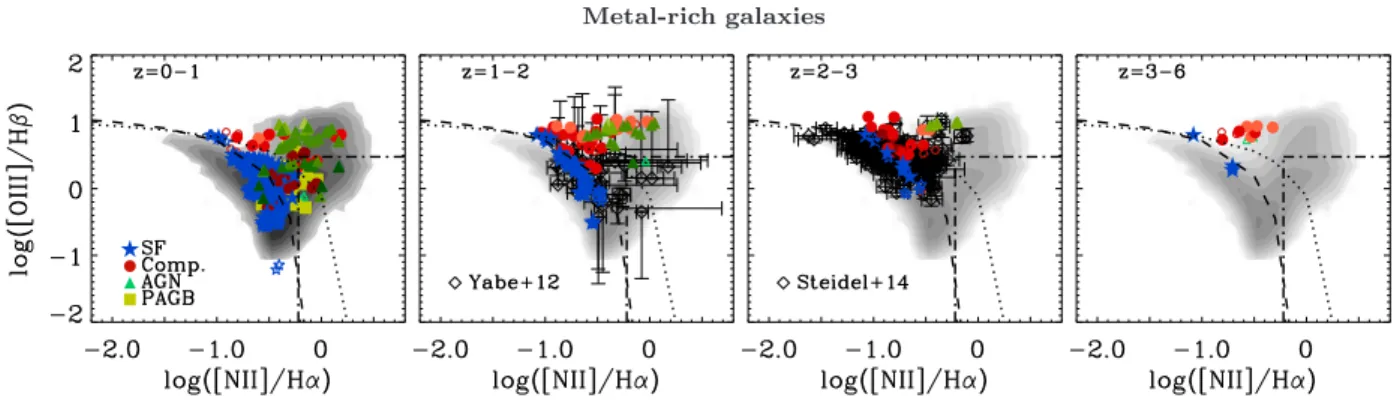
Metal-rich galaxies
Figure 3.Same as Fig.1, but for metal-rich galaxies (N2O2 > −0.8), and including all galaxy types in a single diagnostic diagram in each redshift interval.
galaxies with N2O2 > −0.8 or N3O3 > −0.7 (horizontal red dashed lines) have on average interstellar metallicities above
approximately half solar [log(Zgas,glob/Z⊙) & −0.25].
Fig. 3shows the analogue of Fig. 1after pre-selecting
metal-rich galaxies using the criterion N2O2 > −0.8 (all galaxy types in a given redshift bin are displayed in a same
panel in Fig. 3). In this case, despite the low statistics of
metal-rich galaxies at redshift z > 1, SF-dominated and ac-tive (composite and AGN-dominated) galaxies appear to be graphically separated by the optical selection criterion of
Kewley et al.(2001, black dashed line). Yet, even when pre-selecting metal-rich galaxies, standard optical selection cri-teria still fail to differentiate between composite and AGN-dominated galaxies.
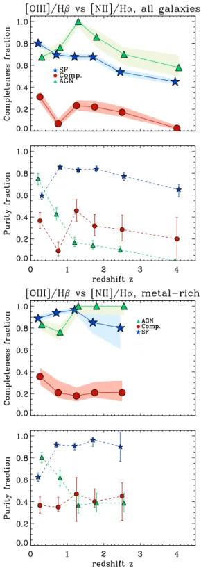
3.3 Purity and completeness fractions for
optically selected galaxy types
From the previous paragraphs, we conclude that standard optical selection criteria can help better distinguish the main ionizing sources in galaxies out to high redshifts when pre-selecting metal-rich galaxies. In this subsection, we further quantify the differentiability of galaxy types with optical selection criteria over cosmic time by computing ‘complete-ness’ and ‘purity’ fractions of SF-dominated, composite and AGN galaxies. The completeness (purity) fraction provides a measure of how complete (uncontaminated) a population of a given observationally selected galaxy type is with respect to our theoretically defined galaxy types. Specifically:
• The completeness fraction is computed by first selecting galaxies of a given type according to the theoretical defini-tion, and then checking how many of these selected galaxies would be classified of the same type according to the obser-vational selection criterion.
• In turn, the purity fraction is calculated by first select-ing galaxies of a given type observationally, and then check-ing how many of these selected galaxies would be classified of the same type theoretically.
In Fig. 4, we show the purity (small symbols, dashed
lines in the first and third panels) and completeness (large symbols, solid lines in the second and fourth panels) frac-tions of SF-dominated (blue), composite (red) and AGN-dominated (green) galaxies versus redshift, when including all galaxies (top two panels) and only pre-selected,
metal-rich galaxies (bottom two panels). When including all galax-ies, the completeness/purity fractions of SF- and AGN-dominated galaxies drop sharply from & 60 per cent at low redshifts to . 60 per cent at z > 1.0, for the reasons outlined
in Section3.1. The purity/completeness fractions of
compos-ite galaxies never exceed ∼40 per cent. When restricting the sample to metal-rich galaxies, the completeness/purity frac-tions of composite galaxies stay similarly low. In contrast, out to z = 3 (beyond which our sample contains hardly any metal-rich galaxy), SF-dominated galaxies have com-pleteness/purity fractions always in excess of 60/70 per cent. For AGN-dominated galaxies, the completeness fraction can even exceed 80 per cent, but the purity fraction remains low at high redshift. This is because of the difficulty of separat-ing composite from AGN-dominated galaxies in optical
line-ratio diagrams, even at high metallicity (Section3.2). Still,
overall, the results of Fig.4reinforce the visual impression
from Fig. 3 that, at high interstellar metallicity, standard
optical selection criteria in the [O iii]/Hβ–[N ii]/Hα diagram help discriminate between active and inactive galaxies out to high redshift.
4 DIFFERENTIATING IONIZING SOURCES
OF GALAXIES IN UV-LINE DIAGNOSTIC DIAGRAMS
In the previous section, we have seen that optical line-ratio diagnostic diagrams can help distinguish active from inactive galaxies out high redshifts only for metal-rich galaxies. In this section, we explore diagnostic diagrams based on
rest-frame UV emission lines to discriminate between ionizing
sources in metal-poor galaxies at all redshifts. As described
in Section1, our methodology, based on the self-consistent
modelling of SF, composite and AGN-dominated galaxies in a full cosmological framework, can bring new insight over
previous pioneering studies in this area (Feltre et al. 2016;
Nakajima et al. 2018).
In the following subsections, we start by exploring the usefulness of different combinations of UV line ratios
and EW, involving (Section 4.1) or not (Section 4.2) the
He ii λ1640 line, to classify simulated, metal-poor galax-ies with different types of ionizing radiation, as defined
through the theoretical BHAR/SFR ratio (see Section 3).
The He ii λ1640 line is problematic because of the difficul-ties of the photoionisation models in reproducing the profile
Figure 4. Completeness (large symbols, solid lines in the first and third panels) and purity fractions (small symbols, dashed lines in the second and fourth panels) as a function of redshift, for simulated SF-dominated (blue stars and lines), composite (red circles and lines) and AGN-dominated (green triangles and lines) galaxies, as classified observationally using the standard criteria ofKewley et al.(2001) andKauffmann et al.(2003) in the optical [O iii]/Hβ–[N ii]/Hα line-ratio diagram. The top two panels show the results when including all simulated galaxies, and the bottom two panels when including only galaxies preselected to be metal-rich, with interstellar metallicities log(Zgas,glob) & −0.25, using
the criterion N2O2 > −0.8 (bottom panel). Error bars and shaded areas illustrate binomial errors. See Section3.3for more details.
and strength of this line in observed spectra (see section5.2
for discussion). These diagnostic diagrams allow us to derive selection criteria for different galaxy types (summarised in
Tables1and2). We also quantify the redshift evolution of
the purity and completeness fractions for UV-selected galaxy
types (Section4.3).
In all UV diagrams considered below, we plot the same simulated galaxies in different redshift intervals as plotted
in the optical diagrams of Section3, but including now only
metal-poor galaxies, as pre-selected with N2O2 < −0.8 (i.e.
with metallicities below about half solar; see Section3.2).
Since we focus on such metal-poor galaxies, we neglect any contribution from post-AGB stellar populations to the to-tal nebular emission (this contribution is mostly impor-tant for evolved, metal-rich galaxies at low redshift; see e.g.Hirschmann et al. 2017). By analogy with the case of
optical lines in Section 3, we apply a flux detection limit
of 10−18erg s−1cm−2 to all UV emission lines of simulated
galaxies (note that we typically lose less then 10 per cent of our galaxies, when applying this flux detection limit). We
also apply a detection limit of 0.1 ˚A on UV emission-line
EW.
4.1 UV-line diagnostics of metal-poor galaxies
including He IIλ1640
Fig. 5shows the distribution of SF (blue stars), composite
(red circles) and AGN-dominated (green triangles) galaxies in five UV diagnostic diagrams constructed using a UV line ratio and a UV line EW, in four redshift intervals, z = 0–1, 1–2, 2–3 and 3–6 (from left to right). The diagnostic dia-grams are (from top to bottom):
(i) EW(C iii] λ1908)) versus C iii] λ1908/He ii λ1640 (here-after EW-C3);
(ii) EW(C iv λ1550)) versus C iv λ1550/He ii λ1640 (here-after EW-C4);
(iii) EW(O iii] λ1663) versus O iii] λ1663/He ii λ1640 (here-after EW-O3);
(iv) EW(Si iii] λ1888) versus Si iii] λ1888/He ii λ1640 (here-after EW-Si3); and
(v) EW(N iii] λ1750) versus N iii] λ1750/He ii λ1640 (here-after EW-N3).
For composite and AGN-dominated galaxies, the sym-bols are further colour-coded according to AGN luminosity (as indicated).
For each UV diagnostic diagram shown in each redshift range, we find a fairly clear separability of different galaxy types, with only some minor overlap between SF-dominated galaxies and composite galaxies with faint AGN. This clear differentiability of galaxy types arises primarily from dif-ferences in line ratios, but also in line EW, as most AGN-dominated galaxies have EW larger than reached by SF-dominated (and to a large extent also by composite) galax-ies. The ratio of any of the five (collisionally excited) metal
lines considered in Fig.5to the He ii λ1640 (recombination)
line decreases from SF-dominated, to composite, to AGN-dominated galaxies. This is because of the harder ionizing radiation of accreting BHs compared to stellar populations, which increases the probability of doubly ionizing helium. This hard radiation also makes the EW of high-ionization, collisionally excited metal lines stronger, and more so for
UV diagnostics with 2 different emission lines incl. He IIλ1640
Figure 5.Distribution of simulated metal-poor (N2O2 < −0.8) SF (blue stars), composite (red circles) and AGN-dominated (green trian-gles) galaxies in five UV diagnostic diagrams constructed using a UV line ratio and a UV line EW, in four redshift intervals, z = 0–1, 1–2, 2–3 and 3–6 (from left to right). The diagnostic diagrams are (from top to bottom): (i) EW(C iii] λ1908) versus C iii] λ1908/He ii λ1640; (ii) EW(C iv λ1550) versus C iv λ1550/He ii λ1640; (iii) EW(O iii] λ1663) versus O iii] λ1663/He ii λ1640; (iv) EW(Si iii] λ1888) versus Si iii] λ1888/He ii λ1640; and (v) EW(N iii] λ1750) versus N iii] λ1750/He ii λ1640. For composite and AGN-dominated galaxies, the sym-bols are further colour-coded according to AGN luminosity (as indicated). As in Fig.1, the line ratios of simulated galaxies are shown for two different values of four undetermined parameters (ξd = 0.3, 0.5; mup = 100, 300M⊙; nH,⋆ = 102, 103cm−1; α = −1.4, −2).
Also show in each diagram are the criteria from the top section of Table1to separate SF-dominated from composite (dashed line), and composite from AGN-dominated (dotted line) galaxies. Observations of SF-dominated (Vanzella 2016;Berg et al. 2016;Senchyna et al. 2017;Stark et al. 2015,2014;Erb et al. 2010) and AGN-dominated (Hainline et al. 2011;Talia 2017;Laporte et al. 2017) galaxies are reported in the first two rows, as indicated.
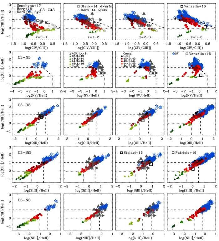
UV diagnostics with 3 different emission lines incl. He IIλ1640
Figure 6. Same as Fig. 5, but for UV diagnostic diagrams constructed using line ratios only. The diagrams are (from top to bottom): (i) C iii] λ1908/He ii λ1640 versus C iii] λ1908/C iv λ1550; (ii) C iii] λ1908/He ii λ1640 versus N v λ1240/He ii λ1640; (iii) C iii] λ1908/He ii λ1640 versus O iii] λ1663/He ii λ1640; (iv) C iii] λ1908/He ii λ1640 versus Si iii] λ1888/He ii λ1640; and (v) C iii] λ1908/He ii λ1640 versus N iii] λ1750/He ii λ1640. Also show in each diagram are the criteria from the middle section of Table1to separate SF-dominated from composite (dashed line), and composite from AGN-dominated (dotted line) galaxies. Observations of dwarf galaxies at z ∼ 0 (Berg et al. 2016;Senchyna et al. 2017) and z = 2–3 (Stark et al. 2014), individual distant SF galaxies (Patr´ıcio et al. 2016;Steidel et al. 2016;Vanzella 2016), Seyfert-2 galaxies at z ∼ 0 and type-2 quasars at z ∼ 2 (Dors et al. 2014) are reported, as indicated.
luminous than for faint AGN. We recall that the EW in
Fig. 5, which account for the emission from narrow-line
re-gions but not for direct attenuated radiation from accreting BHs, should be appropriate for type-2 AGN and taken as
upper limits for type-1 AGN (see Section2.2.4).
Also shown in each panel of Fig.5are proposed
observa-tional selection criteria to separate SF-dominated from com-posite (dashed line), and comcom-posite from AGN-dominated (dotted line) galaxies. These selection criteria, reported in
the top section of Table1, were chosen to maximise the
pu-rity and completeness fractions (Section 4.3). Interestingly,
the same criteria remain valid over the whole redshift range from z = 0 to 6. This indicates that the UV-line ratios and EW of metal-poor galaxies considered here depend far less sensitively on ISM properties than on the nature of the ion-izing radiation.
The EW-C3 and EW-C4 diagrams (first two rows) of
Fig.5also show available observations of dwarf SF galaxies
at z ∼ 0 (Berg et al. 2016;Senchyna et al. 2017) and z =
1.5–4 (Stark et al. 2014), and three SF-dominated galaxies
at z = 2.3, 3.1 and 7 (Erb et al. 2010; Stark et al. 2015;
Vanzella 2016, respectively), along with AGN-dominated
galaxies at z = 2–3, 1.4–4.6 and 7 (Hainline et al. 2011;Talia
2017; Laporte et al. 2017, respectively), as indicated. The predictions from our simulations are in fair agreement with these sparse observational data: observed SF- and AGN-dominated galaxies nicely fall in the regions corresponding to our theoretically defined SF/composite and AGN cate-gories. This agreement with observations corroborates our theoretically derived selection criteria. We note that very high-quality observations will be required to fully exploit
the selection criteria of Fig. 5, which require EW
measure-ments down to 0.1 ˚A.
In Fig 6, we show an alternative to Fig.5constructed
using line ratios only. Specifically, we plot the distribu-tion of SF, composite and AGN-dominated galaxies in five UV diagnostic diagrams constructed each with the C iii] λ1908/He ii λ1640 ratio in ordinate and a ratio involv-ing a third line in abscissa, at different redshifts. The dia-grams are (from top to bottom):
(i) C iii] λ1908/He ii λ1640 versus C iii] λ1908/C iv λ1550 (hereafter C3-C43);
(ii) C iii] λ1908/He ii λ1640 versus N v λ1240/He ii λ1640 (hereafter C3-N5);
(iii) C iii] λ1908/He ii λ1640 versus O iii] λ1663/He ii λ1640 (hereafter C3-O3);
(iv) C iii] λ1908/He ii λ1640 versus Si iii] λ1888/He ii λ1640 (hereafter C3-Si3); and
(v) C iii] λ1908/He ii λ1640 versus N iii] λ1750/He ii λ1640 (hereafter C3-N3).
Irrespective of the redshift range, we obtain a fairly clear separability of different types of metal-poor galaxies in all UV diagnostic diagrams shown.
The clear separability of different galaxy types in
Fig 6 arises from the fact that ratios of
collisionally-excited metal lines to the He ii λ1640 recombination line are highly sensitive to the hard radiation from an AGN,
as described for Fig. 5 above. We note that this is
less the case for N v λ1240/He ii λ1640 (second row), since N v λ1240 requires photons of even higher energy than He ii λ1640 to be produced (77.5 versus 54.4 eV). Hence,
N v λ1240/He ii λ1640 is not a clear indicator of the hardness of the ionizing radiation. In the C3-C43 diagnostic diagram (top row), the C iv λ1550/C iii] λ1908 ratio is also sensitive to the rise of energetic photons from the presence of an AGN, which increases the probability of triply ionizing carbon.
As in Fig. 5, also shown in each panel of Fig. 6 are
proposed observational selection criteria to separate SF-dominated from composite (dashed line), and composite from AGN-dominated (dotted line) metal-poor galaxies. These selection criteria, reported in bottom section of
Ta-ble 1, can be applied over the whole redshift range from
z = 0 to 6.
To compare our theoretical predictions with observa-tions of UV emission lines in active and inactive galaxies, we show, when available, observations from three main
sam-ples in the different panels of Fig. 6, as indicated: (i) a
sample of 22 type-2 AGN assembled by Dors et al. (2014,
and references therein), consisting of 12 Seyfert-2 galaxies in the local Universe and 10 X-ray selected type-2 quasars at redshift 1.5 < z < 4.0; (ii) a sample of five gravita-tionally lensed, low-mass star-forming galaxies at redshifts
1.5 < z < 3.0 fromStark et al. (2014); and (iii) two
sam-ples of dwarf galaxies at z ∼ 0 fromSenchyna et al.(2017)
andBerg et al.(2016). In addition, we show a few individual
distant galaxies fromVanzella(2016),Patr´ıcio et al.(2016)
andSteidel et al.(2016).
We find that observations of SF-dominated galaxies in
Fig. 6 generally overlap with the theoretically defined
SF-galaxy regions (above the dashed line in each panel), but can also fall in the composite-galaxy regions (between dashed and dotted lines). This does not necessarily indicate a mis-match between predictions and observations, as observed SF-dominated galaxies may include a minor contribution from a central accreting BH (or the He ii λ1640 line is not
properly modelled, see section 5.2 for further discussion).
Also, some dwarf-galaxy measurements provide only limits
on emission-line ratios (Stark et al. 2014), compatible with
both composite and SF-dominated model galaxies. Similarly, observations of AGN-dominated galaxies generally overlap
with the theoretically defined AGN regions in Fig.6, but can
also fall in the composite-galaxy regions. This could arise from the contamination of line-flux measurements of AGN narrow-line regions by star formation in the host galaxy
(e.g., Bonzini et al. 2013; Antonucci et al. 2015). We
con-clude that, overall, the sparse observational data currently available are compatible with the UV selection criteria in
Fig.6.
We note that the line measurements shown in Figs.5
and6were not corrected for potential attenuation by dust
in the galaxies. This is not important for the samples of low-mass star-forming galaxies, which have been shown to
be extremely dust-poor (e.g., table 7 ofStark et al. 2014).
For the AGN samples, we prefer not to correct the observed fluxes using an arbitrary attenuation curve, as the dispersion between different standard curves is large at UV wavelengths
(e.g., figure 9 ofCharlot & Fall 2000). Instead, when
com-paring synthetic UV lines with these data, we computed the
attenuation that would be inferred using theCalzetti et al.
(2000) curve for a V -band attenuation of one magnitude
(AV = 1) and found the impact on our analysis to be largely
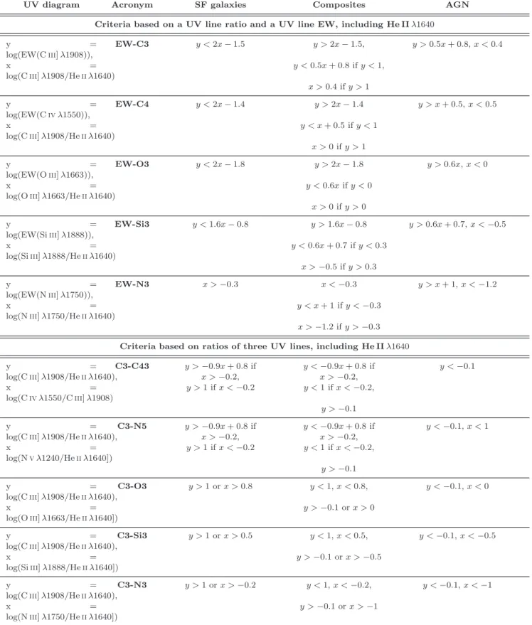
UV diagram Acronym SF galaxies Composites AGN Criteria based on a UV line ratio and a UV line EW, including He IIλ1640
y =
log(EW(C iii] λ1908)),
EW-C3 y < 2x − 1.5 y > 2x − 1.5, y > 0.5x + 0.8, x < 0.4
x =
log(C iii] λ1908/He ii λ1640)
y < 0.5x + 0.8 if y < 1, x > 0.4 if y > 1 y = log(EW(C iv λ1550)), EW-C4 y < 2x − 1.4 y > 2x − 1.4 y > x + 0.5, x < 0.5 x =
log(C iii] λ1908/He ii λ1640)
y < x + 0.5 if y < 1 x > 0 if y > 1 y = log(EW(O iii] λ1663)), EW-O3 y < 2x − 1.8 y > 2x − 1.8 y > 0.6x, x < 0 x =
log(O iii] λ1663/He ii λ1640)
y < 0.6x if y < 0 x > 0 if y > 0 y = log(EW(Si iii] λ1888)), EW-Si3 y < 1.6x − 0.8 y > 1.6x − 0.8 y > 0.6x + 0.7, x < −0.5 x =
log(Si iii] λ1888/He ii λ1640)
y < 0.6x + 0.7 if y < 0.3 x > −0.5 if y > 0.3 y = log(EW(N iii] λ1750)), EW-N3 x > −0.3 x < −0.3 y > x + 1, x < −1.2 x =
log(N iii] λ1750/He ii λ1640)
y < x + 1 if y < −0.3 x > −1.2 if y > −0.3 Criteria based on ratios of three UV lines, including He IIλ1640
y =
log(C iii] λ1908/He ii λ1640),
C3-C43 y > −0.9x + 0.8 if x > −0.2, y < −0.9x + 0.8 if x > −0.2, y < −0.1 x = log(C iv λ1550/C iii] λ1908) y > 1 if x < −0.2 y < 1 if x < −0.2, y > −0.1 y =
log(C iii] λ1908/He ii λ1640),
C3-N5 y > −0.9x + 0.8 if x > −0.2, y < −0.9x + 0.8 if x > −0.2, y < −0.1, x < 1 x = log(N v λ1240/He ii λ1640]) y > 1 if x < −0.2 y < 1 if x < −0.2, y > −0.1 y =
log(C iii] λ1908/He ii λ1640),
C3-O3 y > 1 or x > 0.8 y < 1, x < 0.8, y < −0.1, x < 0
x =
log(O iii] λ1663/He ii λ1640])
y > −0.1 or x > 0
y =
log(C iii] λ1908/He ii λ1640),
C3-Si3 y > 1 or x > 0.5 y < 1, x < 0.5, y < −0.1, x < −0.5
x =
log(Si iii] λ1888/He ii λ1640])
y > −0.1 or x > −0.5
y =
log(C iii] λ1908/He ii λ1640),
C3-N3 y > 1 or x > −0.2 y < 1, x < −0.2, y < −0.1, x < −1
x =
log(N iii] λ1750/He ii λ1640])
y > −0.1 or x > −1
Table 1. Observational selection criteria to discriminate graphically between metal-poor (N2O2 < −0.8) SF-dominated, composite and AGN-dominated galaxies, derived from distributions of simulated galaxies with different BHAR/SFR ratios in the 14 UV/optical diagnostic diagrams of Figs5,6and7. The first column specifies the abscissa and ordinate (EW or line ratio) and the second column the acronym of the diagnostic diagram; the third, fourth and fifth columns the individual selection criteria for SF-dominated, composite and AGN-dominated galaxies, illustrated by the dashed (SF-composite) and dotted (composite-AGN) lines in Figs5and6. See text in Sections4.1and4.2for details.
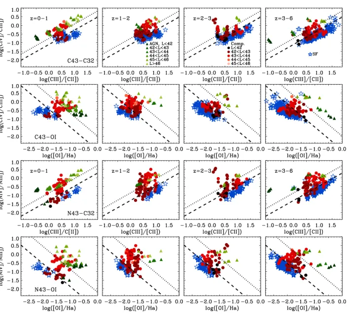
UV diagnostics with 3 or 4 different emission lines without He IIλ1640
Figure 7. Same as Fig.5, but for combined UV/optical diagnostic diagrams not including the He ii λ1640 line. The diagrams are (from top to bottom): (i) C iv λ1550/C iii] λ1908 versus C iii] λ1908/C ii] λ2326; (ii) C iv λ1550/C iii] λ1908 versus [O i]λ6300/Hα; (iii) N iv] λ1485/N iii] λ1750 versus C iii] λ1908/C ii] λ2326; and (iv) N iv] λ1485/N iii] λ1750 versus [O i]λ6300/Hα. Also show in each diagram are the criteria from the bottom section of Table1to separate SF-dominated from composite (dashed line), and composite from AGN-dominated (dotted line) galaxies.
4.2 UV-line diagnostics of metal-poor galaxies not
including He IIλ1640
All the UV-diagnostic diagrams we considered so far to discriminate between ionizing sources in metal-poor galax-ies included the He ii λ1640 line. Recently, problems have arisen when fitting this emission line in observed spectra of local dwarf and high-redshift SF galaxies, using state-of-the-art photo-ionization models combined with (single-star or binary) stellar population synthesis models (e.g.,
Gutkin et al. 2016;Steidel et al. 2016): in some cases, par-ticularly for very metal-poor dwarf galaxies with metallic-ity below 1/5 solar, models can underestimate the observed He ii λ1640-line luminosity by almost an order of magnitude
(e.g., Senchyna et al. 2017; Steidel et al. 2016; Berg et al.
2018;Jaskot & Ravindranath 2016). In this context, the
reli-ability of the UV selection criteria presented in Section4.1to
discriminate between SF-dominated, composite and AGN-dominated metal-poor galaxies may be reduced (see
Sec-tion5.2for a more detailed discussion). To circumvent this
potential drawback, we now present two alternative UV and two combined optical-UV diagnostic diagrams to discrimi-nate between different galaxy types, which avoid the
prob-lematic He iiλ1640 line.
By analogy with Figs5 and 6, we show in Fig.7 the
distribution of SF, composite and AGN-dominated galaxies in four different diagnostic diagrams at different redshifts. The diagrams are (from top to bottom):
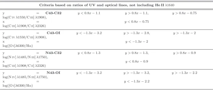
UV diagram Acronym SF galaxies Composites AGN Criteria based on ratios of UV and optical lines, not including He IIλ1640
y =
log(C iv λ1550/C iii] λ1908),
C43-C32 y < 0.8x − 1.1 y > 0.8x − 1.1, y > 0.8x − 0.75
x =
log(C iii] λ1908/C ii] λ2326)
y < 0.8x − 0.75 y = log(C iv λ1550/C iii] λ1908), C43-OI y < −1.3x − 3.2 y > −1.3x − 2.8, y > −1.3x − 2 x = log([O i]λ6300/Hα) y < −1.3x − 2 y =
log(N iv] λ1485/N iii] λ1750),
N43-C32 y < 0.8x − 1.3 y > 0.8x − 1.3, y > 0.8x − 0.9
x =
log(C iii] λ1908/C ii] λ2326)
y < 0.8x − 0.9
y =
log(N iv] λ1485/N iii] λ1750),
N43-OI y < −1.3x − 3.2 y > −1.3x − 3.2, y > −1.3x − 2.2
x =
log([O i]λ6300/Hα)
y < −1.3x − 2.2
Table 2.Same as in Table 1, but now for diagnostic diagrams not including the He ii λ1640 line (see selection criteria quantified by the dashed (SF-composite) and dotted (composite-AGN) lines in Fig.7).
(hereafter C43-C32);
(ii) C iv λ1550/C iii] λ1908 versus [O i]λ6300/Hα (hereafter C43-O1);
(iii) N iv] λ1485/N iii] λ1750 versus C iii] λ1908/C ii] λ2326 (hereafter N43-C32); and
(iv) N iv] λ1485/N iii] λ1750 versus [O i]λ6300/Hα (hereafter N43-O1).
In all diagrams, different galaxy types fall into differ-ent regions, but generally the separability appears to be less clear in these new diagnostic diagrams without the He ii λ1640 line than in the previous ones including the
He ii λ1640 line (see Figs.5and6).
The C iv λ1550/C iii] λ1908 and
N iv] λ1485/N iii] λ1750 ratios typically increase from
SF-dominated, to composite, to AGN-dominated galaxies and with AGN luminosity, because of the corresponding
larger fraction of highly energetic photons (Section 4.1).
The C iii] λ1908/C ii] λ2326 ratio is less sensitive to the details of the ionizing spectrum at high energies, while the [O i]λ6300/Hα ratio is slightly larger for composite and AGN-dominated galaxies than for SF-dominated galaxies,
for reasons outlined in Hirschmann et al. (2017). A
draw-back of the combined UV-optical diagnostic diagrams in
Fig. 7 is that optical lines of distant galaxies shift beyond
the range of near-infrared spectrographs at z & 6. We note
that replacing [O i]λ6300/Hα by [S ii]λ6724/Hα in Fig. 7
would result in a similar separability between different galaxy types. We also found that many other UV line-ratio combinations without the He ii λ1640 line, for example Si iv λ1400/Si iii] λ1888 and Si iii] λ1888/Si ii] λ1814, cannot help discriminate between ionizing sources in galaxies.
As in Figs5and6, we propose in each panel of Fig.7two
observational selection criteria to separate SF-dominated from composite (dashed line), and composite from AGN-dominated (dotted line) metal-poor galaxies. These selection
criteria are reported in Table2. We could not find any
read-ily available observations in the literature to test/validate these criteria.
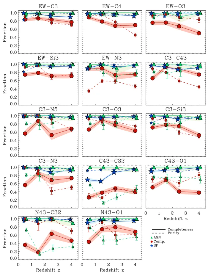
4.3 Purity and completeness fractions for
UV-selected galaxy types
In the previous two subsections, we identified 14 UV diag-nostic diagrams to graphically distinguish between different galaxy types via observational selection criteria reported in
Tables1and 2. In this section, we investigate the
reliabil-ity of these UV selection criteria by computing the corre-sponding completeness and purity fractions, as defined in
Section3.3.
Fig. 8 shows the completeness (large symbols, solid
lines) and purity (small symbols, dashed lines) fractions of SF-dominated (blue), composite (red) and AGN-dominated (green) galaxies versus redshift, as selected using the
crite-ria in Figs 5–7. The 14 panels correspond to the 14
differ-ent diagnostic diagrams of Figs 5–7. In all cases, the
pu-rity/completeness fractions of SF-dominated galaxies and the completeness fraction of AGN-dominated galaxies stay mostly above 90 per cent over the entire redshift range (ex-cept for C43-C32). This indicates that our proposed UV se-lection criteria work remarkably well to select SF-dominated galaxies, and complete samples of AGN-dominated galaxies, from the simulation galaxy sample.
For the EW-C3, EW-C4, EW-O3, EW-Si3 diagrams, the selected AGN samples are in addition largely uncon-taminated by other galaxy types (in particular, composites), as indicated by AGN purity fractions in excess of 90 per cent. The EW-N3, C43, N5, O3, Si3, and C3-N3 diagrams also provide fairly high AGN purity fractions, above 75 per cent. In contrast, for the C43-C32, C43-OI, N43-C32 and N32-O1 diagrams not including the He ii λ1640 line, AGN purity fractions can drop fairly low, down to only 20 per cent, as a consequence of contamination by composite galaxies.
Figure 8. Purity (small symbols, dashed lines) and completeness (large symbols, solid lines) fractions as a function of redshift, for simulated metal-poor (N2O2 < −0.8) SF-dominated (blue stars and lines), composite (red circles and lines) and AGN-dominated (green triangles and lines) galaxies, as classified observationally using the UV selection criteria of Table1. Each panel corresponds to a different UV diagnostic diagram from Figs5,6and7, as indicated at the top.
![Figure 1. [O iii ]/Hβ versus [N ii ]/Hα diagrams for all simulated galaxies and their main high-redshift progenitors in different redshift intervals (different columns)](https://thumb-eu.123doks.com/thumbv2/123doknet/14784356.598062/7.892.86.788.154.619/diagrams-simulated-galaxies-redshift-progenitors-different-intervals-different.webp)
![Figure 2. 2D-Histograms of the optical line ratios N2O2 [≡ log([N ii ]λ6584/[O ii ] λ3727), top panel] and N3O3 [≡](https://thumb-eu.123doks.com/thumbv2/123doknet/14784356.598062/8.892.90.387.146.631/figure-d-histograms-optical-line-ratios-log-panel.webp)