HAL Id: hal-00316848
https://hal.archives-ouvertes.fr/hal-00316848
Submitted on 1 Jan 2001
HAL is a multi-disciplinary open access
archive for the deposit and dissemination of
sci-entific research documents, whether they are
pub-lished or not. The documents may come from
teaching and research institutions in France or
abroad, or from public or private research centers.
L’archive ouverte pluridisciplinaire HAL, est
destinée au dépôt et à la diffusion de documents
scientifiques de niveau recherche, publiés ou non,
émanant des établissements d’enseignement et de
recherche français ou étrangers, des laboratoires
publics ou privés.
On the longitudinal structure of the transient day-to-day
variation of the semidiurnal tide in the mid-latitude
lower thermosphere ? I. Winter season
E. G. Merzlyakov, Yu. I. Portnyagin, C. Jacobi, N. J. Mitchell, H. G. Muller,
A. H. Manson, A. N. Fachrutdinova, W. Singer, P. Hoffmann
To cite this version:
E. G. Merzlyakov, Yu. I. Portnyagin, C. Jacobi, N. J. Mitchell, H. G. Muller, et al.. On the
longitu-dinal structure of the transient day-to-day variation of the semidiurnal tide in the mid-latitude lower
thermosphere ? I. Winter season. Annales Geophysicae, European Geosciences Union, 2001, 19 (5),
pp.545-562. �hal-00316848�
Annales Geophysicae (2001) 19: 545–562 c European Geophysical Society 2001
Annales
Geophysicae
On the longitudinal structure of the transient day-to-day variation
of the semidiurnal tide in the mid-latitude lower thermosphere –
I. Winter season
E. G. Merzlyakov1, Yu. I. Portnyagin1, C. Jacobi2, N. J. Mitchell3, H. G. Muller4, A. H. Manson5, A. N.
Fachrutdinova6, W. Singer7, and P. Hoffmann7
1Institute for Experimental Meteorology, Obninsk, Russia 2Institute for Meteorology, University of Leipzig, Germany 3Department of Physics, University of Wales, Aberystwyth, UK 4Cranfield University, RMCS Shrivenham, Swindon, UK
5Institute for Space and Atmospheric Studies, University of Saskatchewan, Saskatoon, Canada 6Radiophysics Department, Kazan University, Russia
7Institute of Atmospheric Physics, K¨uhlungsborn, Germany
Received: 28 July 2000 – Revised: 26 February 2001 – Accepted: 6 March 2001
Abstract. The longitudinal structure of the day-to-day
vari-ations of semidiurnal tide amplitudes is analysed based on coordinated mesosphere/lower thermosphere wind measure-ments at several stations during three winter campaigns. Pos-sible excitation sources of these variations are discussed. Special attention is given to a nonlinear interaction between the semidiurnal tide and the day-to-day mean wind varia-tions. Data processing includes the S-transform analysis which takes into account transient behaviour of secondary waves. It is shown that strong tidal modulations appear dur-ing a stratospheric warmdur-ing and may be caused by aperiodic mean wind variations during this event.
Key words. Meteorology and atmospheric dynamics
(mid-dle atmosphere dynamics; waves and tides)
1 Introduction
The presence of subsidiary components close to tidal pe-riods is frequently observed in the wind variations in the mesosphere and lower thermosphere (Manson et al., 1982; Cevolani and Kingsley, 1992). These components result in the appearance of oscillations in tidal amplitude and phase. For example, Bernard (1981) showed that variations of tidal parameters with periods of few days are often observed. Specifically, he noticed that tidal fluctuations over a 6 day period are correlated between Garchy (47◦N) and Kiruna (68◦N), but that short-period fluctuations are uncorrelated.
Correspondence to: E. G. Merzlyakov
Based on some theoretical investigations, Bernard sugges-ted that long-period (longer than a few days) variations are related to variations of a tidal excitation source or of propa-gation conditions in the middle atmosphere, whereas short-time (less than a few days) fluctuations may occur due to lo-cal perturbations. Teitelbaum and Vial (1991) suggested that some observations might be explained by nonlinear interac-tions between tides and planetary waves, whose periods are equal to those of the tidal modulations. In recent years, sev-eral authors considered the tidal modulations excited by the nonlinear interaction with planetary waves (Mitchell et al., 1996; Beard et al., 1997, 1999; Kamalabadi et al., 1997; Ja-cobi, 1999; Pancheva and Mukhtarov, 2000). Due to the long periods involved, to date, only a few studies on the nonlinear interaction of different planetary waves have been carried out (Jacobi et al., 1998; Pancheva et al., 2000).
These works, based on the analysis of wind measurements each performed at only one particular site, did not consider the global longitudinal structure of the tidal modulations. However, both tides and planetary waves are global phe-nomena, with characteristic longitudinal structures. A com-prehensive analysis of waves and tides, and possibly non-linear interactions between them, requires the use of wind data measured simultaneously with radars well distributed in longitude, and preferably at similar latitudes. Unfortu-nately, coordinated campaigns that include a sufficient num-ber of radars are scarce. One of them was the DYANA cam-paign (DYnamics Adapted Network for the Atmosphere) car-ried out in early 1990 (Singer et al., 1994; Portnyagin et al., 1994). Another one was carried out under INTAS (Interna-tional Association for the promotion of cooperation with
sci-546 E. G. Merzlyakov et al.: The longitudinal structure of the semidiurnal tide in the mid-latitude lower thermosphere
Obninsk
Volgograd
Kazan
zonal component
meridional component
Obninsk
Volgograd
Kazan
zonal component
meridional component
Obninsk
Volgograd
Kazan
zonal component
meridional component
Obninsk
Volgograd
Kazan
zonal component
meridional component
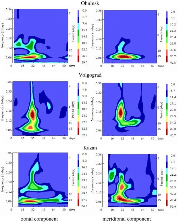
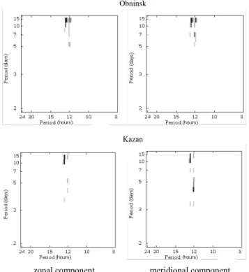
Fig. 1. S-transform spectrograms of semidiurnal tide amplitudes for the Eastern European sites. The days are numbered starting from 1 January 1990. The bar indicates values of squared amplitudes in m2s−2.
entists from the New Independent States of the former Soviet Union) grant 96–1669 in winter 1998/1999.
This investigation considers the longitudinal structure of the long-period day-to-day variations of tidal amplitude. Three periods of observations are investigated. The first one is the DYANA campaign (January–March, 1990). The sec-ond campaign covers the period December 1990 – Febru-ary 1991. The third campaign was carried out in December
1998 within the framework of INTAS grant 96–1669. Our main goals are to show that the tidal modulations are tary scale oscillations and that they are correlated with plane-tary scale oscillations of the mesosphere/lower thermosphere (MLT) mean wind.
Usually the main variation of the mesosphere/lower ther-mosphere wind, at time scales below that of planetary waves, relates to a superposition of the daily mean wind and the
E. G. Merzlyakov et al.: The longitudinal structure of the semidiurnal tide in the mid-latitude lower thermosphere 547
Kühlugsborn
Sheffield
Saskatoon
zonal component
meridional component
Kühlugsborn
Sheffield
Saskatoon
zonal component
meridional component
Kühlugsborn
Sheffield
Saskatoon
zonal component
meridional component
Kühlugsborn
Sheffield
Saskatoon
zonal component
meridional component
Kühlugsborn
Sheffield
Saskatoon
zonal component
meridional component
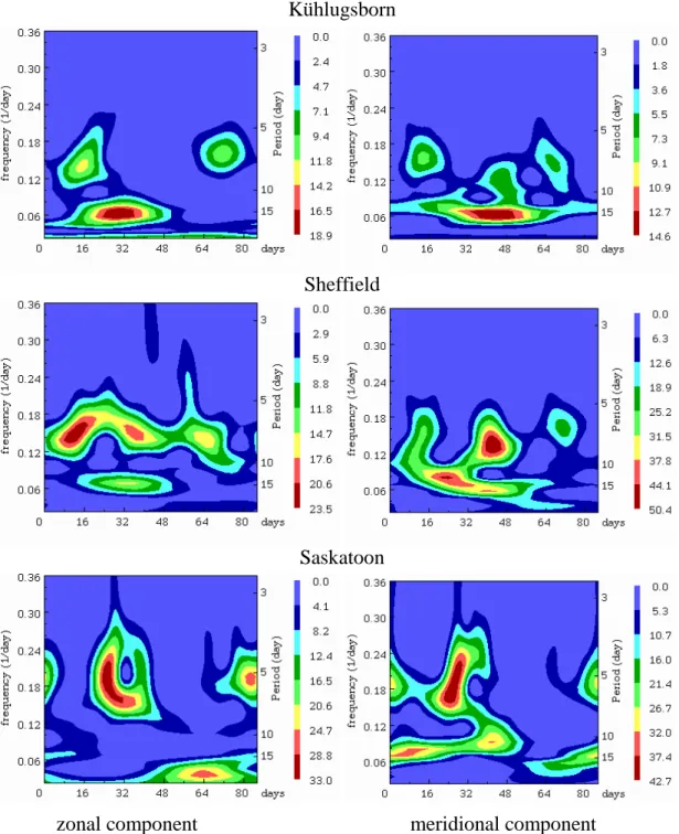
Fig. 2. As Fig. 1, but for the Western European sites.
tides. We will use in this study the term “tidal modulations” (or “modulations”) instead of “day-to-day oscillations in tidal amplitudes”, and the term “mean wind oscillations” instead of “day-to-day oscillations in the mean wind”. It is worth-while to note that we will treat the modulation as a wave. For example, we will estimate a zonal wave number and a direc-tion of propagadirec-tion for the moduladirec-tion. This simplified treat-ment of the modulation would be useful when we consider an
oscillation in the mean wind as a cause of tidal modulations.
2 Measurements and data analysis
The initial data set analysed contains the hourly-mean MLT wind velocity values obtained during the three campaigns. This set is converted to 4-hourly mean values for tidal
pa-548 E. G. Merzlyakov et al.: The longitudinal structure of the semidiurnal tide in the mid-latitude lower thermosphere zonal meridional zonal meridional Amplitude (m/s) Height (km) 74 78 82 86 90 94 98 102 106 1 2 3 4 5 6 7 8 9 10 Saskatoon Kazan zonal meridonal zonal meridional
15-day modulation of tide, Saskatoon and Kazan
Phase (radian) Height (km) 74 78 82 86 90 94 98 102 106 0 1 2 3 4 5 6 Kazan Saskatoon zonal component meridional component Phase (radian) Height (km) 74 78 82 86 90 94 98 102 -1 0 1 2 3 4 5
Vertical structure of the 15-day oscillation in the mean wind over Saskatoon
meridional component zonal component Vertical structure of the 7-day oscillation
in the mean wind over Saskatoon
Phase (radian) Height (km) 76 80 84 88 92 96 100 104 -3.5 -2.5 -1.5 -0.5 0.5 1.5 2.5 3.5 zonal meridional zonal meridional Amplitude (m/s) Height (km) 74 78 82 86 90 94 98 102 106 0 2 4 6 8 10 12 14 Saskatoon Kazan zonal meridional zonal meridional
7 day modulation of tide, Saskatoon and Kazan
Phase (radian) Height (km) 74 78 82 86 90 94 98 102 106 1 1.5 2 2.5 3 3.5 4 4.5 5 5.5 Saskatoon Kazan zonal meridional zonal meridional Amplitude (m/s) Height (km) 74 78 82 86 90 94 98 102 106 1 2 3 4 5 6 7 8 9 10 Saskatoon Kazan zonal meridonal zonal meridional
15-day modulation of tide, Saskatoon and Kazan
Phase (radian) Height (km) 74 78 82 86 90 94 98 102 106 0 1 2 3 4 5 6 Kazan Saskatoon zonal component meridional component Phase (radian) Height (km) 74 78 82 86 90 94 98 102 -1 0 1 2 3 4 5
Vertical structure of the 15-day oscillation in the mean wind over Saskatoon
meridional component zonal component Vertical structure of the 7-day oscillation
in the mean wind over Saskatoon
Phase (radian) Height (km) 76 80 84 88 92 96 100 104 -3.5 -2.5 -1.5 -0.5 0.5 1.5 2.5 3.5 zonal meridional zonal meridional Amplitude (m/s) Height (km) 74 78 82 86 90 94 98 102 106 0 2 4 6 8 10 12 14 Saskatoon Kazan zonal meridional zonal meridional
7 day modulation of tide, Saskatoon and Kazan
Phase (radian) Height (km) 74 78 82 86 90 94 98 102 106 1 1.5 2 2.5 3 3.5 4 4.5 5 5.5 Saskatoon Kazan
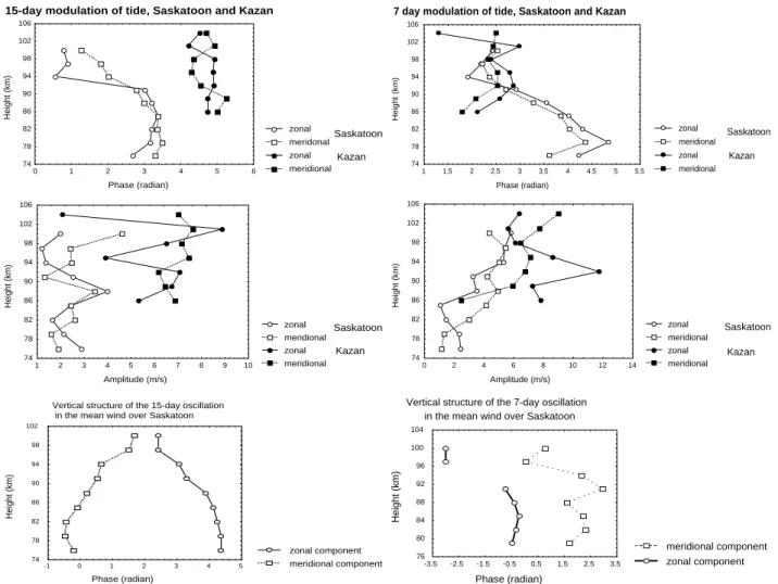
Fig. 3. Vertical profiles of the (a) 15-day and (b) 7-day modulations. The time interval used for calculation is centred at 31 January.
rameters, as described below. The sites involved in the anal-ysis are given in Table 1 for each campaign. Most of the measurements are carried out by meteor radar (MR in Ta-ble 1) and low-frequency (LF) windprofiler data at Collm, Germany (e.g. Jacobi et al., 1998), as well as medium fre-quency (MF) radar at Saskatoon, Canada (e.g. Manson and Meek, 1986) was also added in the first campaign. Some of the meteor radars did not have an explicit height finding, but the majority of meteor echoes were found at heights around 90–95 km, so the results for these radars were attributed to that height range. The Collm low-frequency (LF) wind data, due to the absorption of low-frequency radio waves in the daytime ionospheric D-region above 60 km, have daily gaps and, therefore, cannot be analysed by simply applying spec-tral analysis. To obtain information about tides and their variability, regression analysis with height-dependent coef-ficients has to be applied (e.g. Jacobi, 1999). However, in order to avoid artifacts due to different methods of anal-ysis, in this investigation, the Collm winds are considered only in the analysis of mean wind oscillations, but not for investigating tidal modulations. The Collm winds were cal-culated by averaging the half-hour wind measurements to the
4-hourly mean winds from the height range of 85–105 km. S-transform analysis (Stockwell et al., 1996) is applied to the wind and the semidiurnal amplitude data to reveal the tran-sient nature of the fluctuations. The S-transform is closely related to the continuous wavelet transform and allows one to determine the absolute phase of an oscillation. The signif-icance level of peaks obtained by using the S-transform may be estimated according to a method presented by Portnyagin et al. (2000). To obtain the 4-hourly mean parameters of the semidiurnal tide a sliding harmonic analysis was performed on 48 hour and 72 hour intervals of the hourly-mean wind velocities. The choice of 4-hourly mean data is based on a convenience of the data processing by our realisation of the S-transform analysis. The 72 hour intervals were used only for the processing of the DYANA data inorder to reduce er-rors of the tidal parameters. Before applying the S-transform, some data gaps were interpolated by a second degree poly-nomial fit. In the output of the S-transform analyses, we obtain the time-varying power spectrum and phase distribu-tion of the moduladistribu-tions. Thus, longitudinal and vertical (at Saskatoon and Kazan, where height finding was available) structures of the modulations may be considered. Before
de-E. G. Merzlyakov et al.: The longitudinal structure of the semidiurnal tide in the mid-latitude lower thermosphere 549 Kühlungsborn
Sheffield
zonal component meridional component
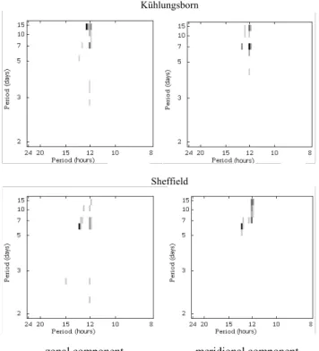
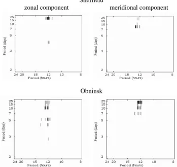
Fig. 4. Bispectra estimated for the hourly wind data of the Western European sites. Data time interval covers 1024h from first days of January.
termining the longitudinal and vertical modulation structure, the time interval, during which the amplitudes of the mod-ulations have simultaneously relatively large values at every site, has to be specified from the time series of the power spectra at each site. Inside this interval, one time is selected to estimate phases and amplitudes of the modulations.
For the following comparison of results for different sites, it should be taken into account the time and frequency res-olution of the employed S-transform method. The time of maximum amplitude has an approximate uncertainty of the order of an oscillation period. The frequency of an oscilla-tion is determined with the error of about 16%.
Let ωPW, sPW be a frequency and a zonal wave number of a planetary wave; ωTd, sTd are a frequency and a zonal wave number of tide. As a result of nonlinear interaction between the planetary wave and the tide, or linear interaction between the planetary wave and a tidal source, we will observe two secondary waves with frequencies and zonal wave numbers,
ωTd±ωPWand sTd±sPW. The same connection is not nec-essarily true for the phases of the oscillations. The particular process that leads to the interaction defines their correspon-dence. To check for the presence of two secondary waves, we used an ordinary periodogram analysis.
Relationships between the frequencies of the modulations and the frequencies of the oscillations in the mean wind were analysed using bispectrum analysis. This method has proved to be a powerful tool for the estimation of nonlinear
interac-tions and has frequently been used for analysing MLT winds in recent years (R¨uster, 1994; Clark and Bergin, 1997; Ka-malabadi et al., 1997; Beard et al., 1999). We used an in-direct method of bispectrum estimate (Chrysostomos et al., 1987) and did not divide an investigated time interval into subrecords. This method permits one only to reach a con-clusion about the correspondence of the frequencies in ac-cordance with the theory of nonlinear interaction; but, as pointed out by Beard et al. (1999), this cannot be consid-ered as real proof of a non-linear process actually occurring. However, when investigating time series that are relatively short with respect to the periods to be investigated, subdivid-ing the time series would result in too great a loss of spectral resolution. One possible way to estimate the significance of a bispectrum result is a check of the hypothesis that the data set was obtained from the Gaussian noise (Haubrich, 1965). Such a procedure, though, is not suitable for the analysis of MLT wind time series, because the semidiurnal tidal signa-ture on the time series will imprint a distinct non-Gaussian distribution to the wind statistics. Therefore, a Monte-Carlo simulation was carried out to evaluate the significance level of the obtained bispectrum results. An artificial record with a length of 1024 hours, containing a sum of a semidiurnal tide and a normally (0, σ ) distributed noise, was constructed and the bispectra were calculated for 100 independent records. This will be a sufficiently large number for accurate estima-tion of the significance level, which was tested for one se-lected case using an extended number of 1000 records. Thus, the probability distribution of the maximum response in the bispectrum was estimated. For each site, the artificial noise in the records was estimated in relation to the amplitude of the semidiurnal tide, and this ratio was taken from the mea-surements at these sites.
Let ω1and ω2be the positive frequencies of two secondary
waves observed in one wind direction. We may represent the oscillations in this direction as
A1cos(ω1t + s1λ + ϕ1) + A2cos(ω2t + s2λ + ϕ2)
+ATdcos(ωTdt + sTdλ + ϕTd), (1) where λ is the longitude, A1, A2, ATdand ϕ1, ϕ2, ϕTdare the amplitudes and initial phases of the secondary waves and the tide, respectively. When we extract the information about the tide by applying harmonic analysis, we obtain, assuming
|ω1−ωTd| ωTdand |ω2−ωTd| ωTd, an expression for the apparent tidal amplitude A:
A2=A2Td+A21+A22 +2ATdA1cos [(ω1−ωTd) t + (s1−sTd) λ + ϕ1−ϕTd] +2ATdA2cos [(ω2−ωTd) t + (s2−sTd) λ + ϕ2−ϕTd] +2A1A2cos [(ω1−ω2) t + (s1−s2) λ + ϕ1−ϕ2] (2)
In the expression (2), non-significant terms are omitted. Thus, it is appropriate to operate with the squared amplitudes of
550 E. G. Merzlyakov et al.: The longitudinal structure of the semidiurnal tide in the mid-latitude lower thermosphere Obninsk
Kazan
meridional component zonal component
Fig. 5. As Fig. 4, but for the Eastern European sites.
the tide to investigate the modulations. However, the ampli-tude of the modulation is generally smaller than that of the tide and is about 30–50% of monthly mean tidal amplitude, i.e. the squared modulation amplitude is equal or less than a quarter of the squared tidal amplitude. We have performed the calculations with the squared amplitudes and have ob-tained the same results related to the frequencies and zonal wave numbers of the modulations as those for the unchanged amplitudes. As it can also be seen, the modulation of tidal amplitude is a result of superposition of two oscillations. When the secondary waves propagate to the point of obser-vation under different atmospheric conditions, the final lon-gitudinal phase distribution of the modulation would be dis-torted. Theoretically, there are possibly short-period normal mode waves in the atmosphere (Hamilton et al., 1986), which may be excited by global strong variations in the atmospheric parameters (e.g. during stratospheric warming events). The periods of some normal mode waves are close to the tidal pe-riod of 12 hours and they can be confused with the secondary waves. Thus, it is difficult to reveal the normal mode waves in the wind measurements. However, there is a possibility that these waves can also distort the longitudinal phase dis-tribution of the modulation. Additionally, we have to keep in mind the existence of a lunar semidiurnal tide that can mod-ulate the solar semidiurnal tide with the period of about 15 days and with a zonal wave number 0. When there is no addi-tional distortion, we obtain a similar phase distribution of the modulation for both zonal and meridional tidal components. Moreover, if the secondary wave has the same polarisation of horizontal velocity as the tide (e.g. nonlinear interaction),
zonal component meridional component Phase distribution on longitude for the 15-day tidal modulation
Longitude (radian) Phase (radian) -2.5 -1.5 -0.5 0.5 1.5 2.5
-2.2 -1.6 -1 -0.4 0.2 0.8 1.4 15-day mean wind
oscillation
zonal component meridional component
Phase distribution on longitude for the 7-day tidal modulation
Longitude (radian) Phase (radian) -3 -1 1 3 5 7 9
-2.2 -1.6 -1 -0.4 0.2 0.8 1.4 7-day mean wind
oscillation
Fig. 6. Longitudinal structures of the tidal modulations and of zonal components of the mean wind oscillations.
we can expect the values of phase for different components to be close to each other.
Actually, the source of secondary waves may depend on the local amplitudes of tide and planetary waves. However, we focus our analysis only on those secondary waves which reveal their global character. There are several numerical simulations of secondary waves, resulting from the interac-tion between the semidiurnal tide and planetary waves. They definitely demonstrate global vertical and horizontal propa-gation of the secondary waves from the source region (e.g. Palo et al., 1999).
3 Results and discussion
3.1 The DYANA campaign
The main characteristics of the prevailing wind and semid-iurnal tide during the DYANA campaign were presented in studies of Singer et al. (1994) and Portnyagin et al. (1994). Particularly, it was shown that the most intensive day-to-day variations of the mean wind are related to the period of the stratospheric warming that occurred during the campaign, and that there are also long-period tidal modulations dur-ing the DYANA campaign. The S-transform analysis gives more exact and definite results and confirms these conclu-sions. Figs. 1 and 2 show the distributions of the modulation frequencies with time. The data are calculated from winds at 95 km altitude (for Saskatoon at 94 km). The days are
E. G. Merzlyakov et al.: The longitudinal structure of the semidiurnal tide in the mid-latitude lower thermosphere 551
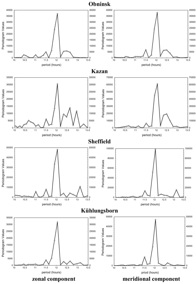
Obninsk
period (hours) P er iodogr am V al ues 0 5000 10000 15000 20000 25000 30000 35000 40000 0 5000 10000 15000 20000 25000 30000 35000 40000 10 10.5 11 11.5 12 12.5 13 13.5 period (hours) P er iodogr am V al ues 0 5000 10000 15000 20000 25000 30000 35000 40000 0 5000 10000 15000 20000 25000 30000 35000 40000 10 10.5 11 11.5 12 12.5 13 13.5Kazan
period (hours) P eriodogram V alues 0 5000 10000 15000 20000 25000 30000 35000 0 5000 10000 15000 20000 25000 30000 35000 10 10.5 11 11.5 12 12.5 13 13.5 period (hours) P eriodogram V alues 0 10000 20000 30000 40000 50000 60000 70000 0 10000 20000 30000 40000 50000 60000 70000 10 10.5 11 11.5 12 12.5 13 13.5Sheffield
period (hours) P e ri odogr am V a lues 0 10000 20000 30000 40000 50000 0 10000 20000 30000 40000 50000 10 10.5 11 11.5 12 12.5 13 13.5 period (hours) Per iodogr am Val ues 0 20000 40000 60000 80000 100000 0 20000 40000 60000 80000 100000 10 10.5 11 11.5 12 12.5 13 13.5Kühlungsborn
period (hours) P er iodogr am V al ues 0 5000 10000 15000 20000 25000 30000 35000 0 5000 10000 15000 20000 25000 30000 35000 10 10.5 11 11.5 12 12.5 13 13.5 priod (hours) Per iodogr am Val ues 0 10000 20000 30000 40000 50000 0 10000 20000 30000 40000 50000 10 10.5 11 11.5 12 12.5 13 13.5zonal
component
meridional
component
552 E. G. Merzlyakov et al.: The longitudinal structure of the semidiurnal tide in the mid-latitude lower thermosphere
zonal direction
meridional direction
a)
b)
c)
d)
10hPa 30hPa Dh in km -1 -0.4 0.2 0.8 1.4 2 2.6 0 16 32 48 64 80
10hPa 30hPa -90 -80 -70 -60 -50 -40 -30 -20 -10 0 16 32 48 64 80 tem p erature in oC
Kü hl ugs bo rn
Sheffi el d
Sask atoo n
z o nal co mp o n ent
mer i d io na l co mp o n ent
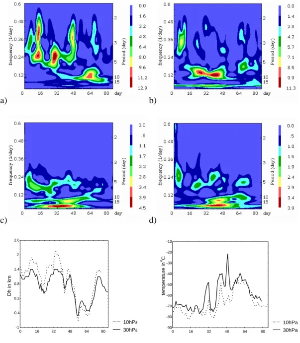
Fig. 8. Cross S-transform spectrograms of the winter 1990–1991 campaign for the mean winds (a and b) and for semidiurnal tide amplitudes (c and d). At the bottom the depth of the polar vortex (left) and the polar temperature (right) are shown at two height levels: 10 hPa and 30 hPa.
numbered, starting from 1 January 1990. As seen from the figures, there are modulations with common periods for all stations at the same time. The difference between the re-sults for meridional and zonal components within each site is smaller than those between the different sites. The common significant modulations with periods of about 15 days and 7 days can clearly be detected at different globally distributed sites. As an exception, at Saskatoon, the zonal component of the 15-day modulation is very weak, but it is also signif-icant at both lower and upper heights at this site (not shown here). At the same time, the meridional component of the
15-day modulation is quite strong at Saskatoon. Compari-son of Figs. 1 and 2 took into account the time and period resolution of the S-transform. Figure 3 illustrates vertical structures of the 15- day and 7-day modulations for Saska-toon and Kazan, where height finding was available. The figure shows profiles of amplitudes and phases of the respec-tive oscillations, with the data window centred at 31 January. For comparison, in the lowermost panels, the vertical struc-ture of the 15-day and 7-day oscillations of the daily mean wind at Saskatoon is added. In this figure, the large ver-tical wavelength of the modulations is seen from the small
E. G. Merzlyakov et al.: The longitudinal structure of the semidiurnal tide in the mid-latitude lower thermosphere 553 phase gradient between 86 and 100 km over Kazan. The tidal
modulations observed at Saskatoon also indicate large verti-cal wavelengths at the lower layers, but a phase shift around 90 km. The figure demonstrates very similar behaviour of the phases for the zonal and meridional components of the mod-ulations. This is significantly different from the behaviour of the phases for the oscillation in the mean wind for which the vertical structures of the meridional and zonal components are different. From Fig. 3, one can see that the 15-day os-cillation in the zonal component of the mean wind has the same vertical structure as the 15-day modulation; the same is true for Kazan. This result is not shown here because the vertical phase distributions of the modulations and the mean zonal wind oscillations for Kazan are very similar.
The estimated bispectra of hourly-mean data are shown in Figs. 4 and 5. These bispectra are scaled in such a way that the respective darkest point has a confidence level greater than 95%. Note that the scaling of the two axes is differ-ent; this is necessary to take into account the wide period difference between frequencies of the day-to-day mean wind oscillations and frequencies of wind oscillations with the pe-riods close to 12 hours. In the bispectra for the K¨uhlungsborn data, significant responses relate to an interaction of oscilla-tions with periods near 12 hours and 15-days for both compo-nents of the mean wind. There is also a significant response for the point near (12 hours and 7 days) for the meridional component of the mean wind. The significant responses in the bispectra for the Sheffield data relate to an interaction of the 6-day oscillation and the semidiurnal tide, resulting in a 13 hour oscillation, which is visible in both components of the mean wind. Also, there is a significant response for the meridional components of the 14-day oscillation and the semidiurnal tide. The bispectra for the Obninsk data have significant responses in both components of the 15-day cillation and the semidiurnal tide, resulting in secondary os-cillations close to 12 hours. There is also the significant re-sponse for the meridional components of the 7-day oscilla-tion and the semidiurnal tide. For the Kazan data, there are significant responses only for the 14-day oscillation and an oscillation with a period close to 12 hours, which, however, also indicates that the semidiurnal tide is involved. Taking into account the transient nature of the secondary waves, we may conclude that the bispectra indicate a possible involve-ment of the semidiurnal tide and of the 15-day and 7-day oscillations of the mean wind into the nonlinear interaction.
Nonlinear interaction of waves and tides results in a mod-ulation of the latter, with the period of the former, and this modulation also exhibits the same longitudinal structure as the original waves. The distributions of phases of the semid-iurnal tide modulation with longitude are shown in Fig. 6 to show their longitudinal structure, in particular, with respect to their zonal wave numbers. The lines in Fig. 6 are the re-sults of a least squares fit and have the slopes (i.e. the zonal wave numbers) of about −2 for the 7-day modulations and
−1.5 (zonal component) or −2 (meridional component), re-spectively, for the 15-day modulations. Here, and in the rest of the paper, a positive zonal wave number corresponds to
Sheffield
zonal component meridional component
Obninsk
Fig. 9. Bispectra estimated for the hourly wind data of Sheffield and Obninsk.
westward propagation. In the figure, the errors bars are indi-cated for the zonal component. If we accept a hypothesis of the nonlinear interaction between the tide and the planetary waves, then these slopes correspond to an eastward propaga-tion of the primaries planetary waves. However, Portnyagin et al. (1999) have presented a planetary 15-day wave during the DYANA campaign, propagating westward with a zonal wave number 1, and a 7-day planetary wave, observed only in the meridional direction, with a zonal wave number 0. At the moment of maximum tidal modulation, the waves have not yet been formed over all sites and in the meridional mean wind, the 15-day oscillations are in phase for different Euro-pean sites. As shown by Portnyagin et al. (1999), the wave is globally formed in the considered height range, not before early February.
At this stage, the following results may be emphasized: (1) the longitudinal structures of the modulations do not
correspond to those of the planetary waves in the pre-vailing wind;
(2) for the meridional and zonal components of the modu-lations, the values of phases do not differ significantly; (3) the distribution of phases, due to the longitudinal
distri-bution of the measuring sites, shows a tendency to clus-ter in groups on longitude and makes it difficult to ac-curately assess a zonal wave number for these modula-tions. Evidently, a definite estimate of the slopes needs one more site between Saskatoon and Kazan or between Saskatoon and Sheffield.
The nonlinear interaction between a day-to-day mean wind oscillation and semidiurnal tide causes the appearance of two
554 E. G. Merzlyakov et al.: The longitudinal structure of the semidiurnal tide in the mid-latitude lower thermosphere
zonal
component
meridional
component
Sheffield
Period (hours) P eri odogram V al ues 0 5000 10000 15000 20000 25000 30000 35000 0 5000 10000 15000 20000 25000 30000 35000 10 10.5 11 11.5 12 12.5 13 13.5 period (hours) P eri odogram V al ues 0 5000 10000 15000 20000 25000 30000 35000 40000 0 5000 10000 15000 20000 25000 30000 35000 40000 10 10.5 11 11.5 12 12.5 13 13.5Obninsk
period (hours) P eriodogram V alues 0 1000 2000 3000 4000 5000 0 1000 2000 3000 4000 5000 10 10.5 11 11.5 12 12.5 13 13.5period (hours) P e ri odogr am V a lues 0 2000 4000 6000 8000 10000 12000 0 2000 4000 6000 8000 10000 12000 10 10.5 11 11.5 12 12.5 13 13.5
Sheffield – Obninsk
period (hours) Squar ed Coher ency 0 0.2 0.4 0.6 0.8 1 0 0.2 0.4 0.6 0.8 1 10 10.5 11 11.5 12 12.5 13 13.5period (hours) Squar ed Coher ency 0 0.2 0.4 0.6 0.8 1 0 0.2 0.4 0.6 0.8 1 10 10.5 11 11.5 12 12.5 13 13.5
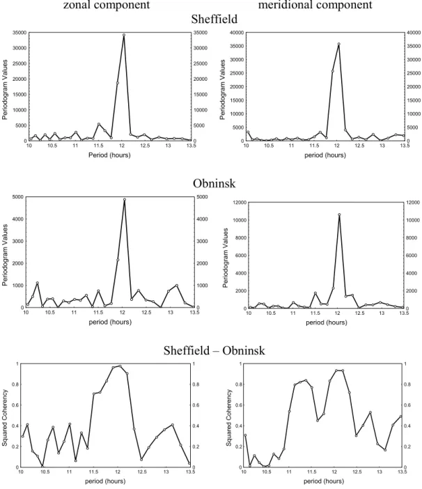
Fig. 10. Periodograms evaluated for the Obninsk and Sheffield hourly wind data. The squared coherency between the hourly winds of Obninsk and Sheffield is shown at the bottom.
secondary waves. Figure 7 shows the periodograms for four stations estimated for the time interval during which the mod-ulations exist. From the theory, one expects to find the fol-lowing side peaks: for a 15-day modulation, 12.4 hours and 11.6 hours, for a 7-day modulation, 11.2 hours and 13 hours. Not all of the peaks are observed simultaneously for each station near the pointed values. However, part of the peaks is visible in the periodogram for one station and the other peaks are visible in the periodogram for another station. This is a consequence of the transient behaviour of the subsidiary waves, while the periodogram shows an average power of
the oscillation over the analysed interval. However, the S-transform analysis cannot show the existence of both sec-ondary waves.
Thus, the indications of the nonlinear interaction between the day-to-day mean wind oscillations and the semidiurnal tide have been revealed and these mean wind oscillations are not related to the global planetary waves for the considered height range.
A short-period normal mode wave with the period 11.6 hours would modulate the tide with a period of 14 days and the zonal wave number of the modulation would be 2
(east-E. G. Merzlyakov et al.: The longitudinal structure of the semidiurnal tide in the mid-latitude lower thermosphere 555 ward propagating). However, a normal mode with a period
of about 12.4 hours does not exist and the semidiurnal tide modulation by a lunar tide has a zonal wave number 0. If one analyses the phase distribution of the 15-day oscillation in the zonal mean wind during the time interval of the mod-ulation (about 28 January – 2 February), one will obtain the same distribution for the zonal component of the 15-day os-cillation, as the one in the 15-day modulation, as shown in Fig. 6. During this time, strong wave-like mean wind vari-ations were observed (Singer et al., 1994). The considered eastward 15-day oscillation may be a part of a frequency band of these variations. Also, the eastward travelling tran-sients are known to appear in the first phase of a stratospheric warming (e.g. from numerical simulation – Geisler, 1974; and from observation – Leovy et al., 1976) and the modula-tion of the semidiurnal tide coincides with this phase during the DYANA campaign. Thus, these transients may modu-late the tide somewhere at lower atmospheric levels. During a warming, the short-period normal mode may also be ex-cited and thus, distorts the phase distribution of the modu-lation. However, the close values of phases for meridional and zonal components point to a weakness of the distortion. Another possible source of the 15-day modulation is a varia-tion of the tidal source due to the eastward transients. For the considered case, this possibility is not in agreement with the behaviour of the modulation over Saskatoon. The secondary waves have periods of oscillations near 12 hours and if they should be forced, their behaviour would be similar to that of the semidiurnal tide. The earlier considered processes may also be responsible for the modulation of the tide with the period of 7 days.
3.2 The Winter 1990–1991 campaign
This period is characterised by the existence of a few weak warmings during January 1991, and a major warming during February. We will consider only long-period modulations of the semidiurnal tide amplitude (about 10–15 days). Figure 8 shows the cross-S-transform results of the Sheffield and Ob-ninsk tidal amplitude data and the mean wind data, starting from 11 December 1990. Alos in this figure, the depth of the polar vortex, defined as the zonal mean pressure level height difference between 60◦N and the pole, and the temperature above the pole, are presented at the height levels 30 hPa and 10 hPa. Near Day 38, the quasi 15-day (10–12 day) and about 21-day oscillations are clearly visible in the tidal amplitude and in the mean wind. As observed during the DYANA cam-paign, these modulations are heading the main stratospheric warming. The zonal wave numbers of the tidal modulations and of the oscillations in the mean wind are the following: about 0.6 ± 0.5 for the zonal component and 3 ± 0.5 for the meridional component of the mean wind; about 1 ± 1 for the zonal component and 2.5±1 for the meridional component of the quasi 15-day modulation near Day 38. The errors in the wave numbers were estimated from a least squared fitting of the data. For the mean wind oscillations the measurements from 3 sites (Table 1) were used, and for the tidal
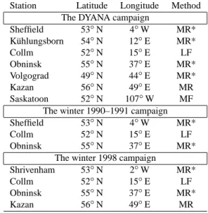
modula-Table 1. Mesosphere/lower thermosphere wind measuring stations considered during the 3 campaigns. The measurements are carried out by meteor radar (MR), low-frequency drift measurements (LF) and medium frequency radar (MF). Measurements without height finding are marked by an asterisk.
Station Latitude Longitude Method The DYANA campaign
Sheffield 53◦N 4◦W MR* K¨uhlungsborn 54◦N 12◦E MR* Collm 52◦N 15◦E LF Obninsk 55◦N 37◦E MR* Volgograd 49◦N 44◦E MR* Kazan 56◦N 49◦E MR Saskatoon 52◦N 107◦W MF The winter 1990–1991 campaign Sheffield 53◦N 4◦W MR* Collm 52◦N 15◦E LF Obninsk 55◦N 37◦E MR*
The winter 1998 campaign
Shrivenham 53◦N 2◦W MR* Collm 52◦N 15◦E LF Obninsk 55◦N 37◦E MR*
Kazan 56◦N 49◦E MR
* – station without height resolution
tions, the data from only 2 sites were used. Thus, in this case, the zonal wave numbers of quasi 15-days modulations and of quasi 15-day oscillations in the mean wind are similar. In Fig. 9, the bispectra are shown for mean hourly data series starting from 24 December. The darkest points have a confidence level greater than 90% for the zonal component and greater than 95% for the meridional component of oscil-lations. The bispectra indicate that the considered oscillation of the mean wind and the tidal amplitude may interact. How-ever, the data do not allow one to distinguish whether this is a result of the linear modulation of a tidal source or of the nonlinear interaction between the wave and the semidiurnal tide. In addition, there is no clearly expressed coincidence between periods of these oscillations in mean wind and tidal modulation, as seen in Fig. 8. This gives evidence against the possibility that we observed the nonlinear interaction locally. The interesting case is 10–12 day modulations near Day 64, when the warming is observed. The phase distribution of 10–12 day oscillation in the zonal mean wind corresponds to a westward propagating wave near this day, while for the modulation, it corresponds to an eastward propagating wave with zonal wave number 2. Figure 10 shows periodogram analyses of the zonal and meridional winds at Sheffield and Obninsk. Only one side peak is present and it has a period of 11.6 hours. In the lowermost panel, the coherency spectrum estimated for hourly mean wind is shown. The coherence at the corresponding frequency is about 0.8, at a confidence level of more than 95%. In this study this is the unique case with a significant coherency. Usually the necessity of high
556 E. G. Merzlyakov et al.: The longitudinal structure of the semidiurnal tide in the mid-latitude lower thermosphere
Obninsk
Shrivenham – Kazan
Collm – Kazan
zonal component
meridional component
Obninsk
Shrivenham-Kazan
zonal component
meridional component
temperature above North pole
Days from December 1, 1998
temperature o C -80 -75 -70 -65 -60 -55 -50 -45 -40 -35 0 8 16 24
Obninsk
Shrivenham-Kazan
zonal component
meridional component
temperature above North pole
Days from December 1, 1998
temperature o C -80 -75 -70 -65 -60 -55 -50 -45 -40 -35 0 8 16 24
Fig. 11a. S-transform results for the December 1998 campaign. Results of tidal amplitudes for Obninsk data (top panel). Cross-S-transform results between the tidal amplitudes of Shrivenham and Kazan (middle panel). In the lowermost panel the 30 hPa temperature above the pole is shown.
resolution does not allow one to obtain large values of the coherency. A possible explanation of the observed case is that the co-existence of the semidiurnal tide and the normal mode wave with the period of 11.6 hours (Hamilton et al., 1986) forms the main part of the apparent tidal variability. This wave has the zonal wave number 0 and would modulate the tide at observed frequency, with a corresponding zonal wave number.
The longest oscillations in the mean wind and in the tidal
amplitude correspond to the longitudinally independent vari-ations of the tide and the mean wind with a period of 21 days. There is no additional indication of the nature of the modu-lation for this case.
3.3 The December 1998 campaign
A rather strong stratospheric warming was observed in the middle of this month. The warming resulted in
simultane-E. G. Merzlyakov et al.: The longitudinal structure of the semidiurnal tide in the mid-latitude lower thermosphere 557
Ob ni nsk
Shri venham
– Kazan
Collm
– Kazan
z o n a l c o m
p o ne nt
m
er i d i on al co m
p o n en t
Obninsk
Shrivenham – Kazan
Collm – Kazan
zonal component
meridional component
Obninsk
Shrivenham – Kazan
Collm – Kazan
zonal component
meridional component
Obninsk
Shrivenham – Kazan
Collm – Kazan
zonal component
meridional component
Obninsk
Shrivenham – Kazan
Collm – Kazan
zonal component
meridional component
Fig. 11b. Spectrograms for the mean wind variations over Obninsk (top panel). Cross-S-transform results for the mean wind data of Shrivenham and Kazan (middle panel) and for the mean wind data of Collm and Kazan (bottom panel).
ous variations of the mean wind and of the semidiurnal tide, with periods of about 12–14 days. This is shown in Fig. 11, where results of S-transforms of the mean winds for Shriven-ham, Collm, Obninsk and Kazan (at 92 km altitude) and the semidiurnal tidal amplitude data at Shrivenham, Obninsk and Kazan are presented. However, it can be seen from Fig. 11 that the modulation of the tide does not occur simultaneously with the mean wind oscillations. The modulations exist near Days 10 and 40 (see results for Shrivenham and Kazan)
num-bered from 1 December 1998, but the wave exists between these days. This means that the modulations of the tidal am-plitude are themselves modulated, too. Possibly there are two main modulations with frequencies close to each other. The broad side bands in the periodograms, presented in Fig. 12, confirm this suggestion.
In Fig. 13, the vertical structure of the mean wind oscilla-tion and of the semidiurnal tidal modulaoscilla-tion, obtained from the S-transform of the Kazan data, are presented for two
pe-558 E. G. Merzlyakov et al.: The longitudinal structure of the semidiurnal tide in the mid-latitude lower thermosphere
zonal component
meridional component
Obninsk
period (hours) Periodogram Values 0 2000 4000 6000 8000 10000 12000 14000 0 2000 4000 6000 8000 10000 12000 14000 10 10.5 11 11.5 12 12.5 13 13.5 period (hours) Periodogram Values 0 5000 10000 15000 20000 25000 30000 0 5000 10000 15000 20000 25000 30000 10 10.5 11 11.5 12 12.5 13 13.5Shrivenham
period (hours) Periodogram Values 0 5000 10000 15000 20000 25000 30000 35000 0 5000 10000 15000 20000 25000 30000 35000 10 10.5 11 11.5 12 12.5 13 13.5period (hours) Periodogram Values 0 10000 20000 30000 40000 50000 60000 70000 0 10000 20000 30000 40000 50000 60000 70000 10 10.5 11 11.5 12 12.5 13 13.5
Kazan
period (hours) Periodogram Values 0 5000 10000 15000 20000 25000 30000 35000 40000 0 5000 10000 15000 20000 25000 30000 35000 40000 10 10.5 11 11.5 12 12.5 13 13.5period (hours) Periodogram Values 0 5000 10000 15000 20000 25000 30000 0 5000 10000 15000 20000 25000 30000 10 10.5 11 11.5 12 12.5 13 13.5
Fig. 12. Periodograms evaluated for the hourly wind data of the winter 1998 campaign.
riods centred at Days 10 and 40. The vertical lengths of the oscillation and the modulation are not in agreement for the first case. The vertical wavelength of the modulation is about 45 km. It proves too short to obtain the true values of phases at sites without height finding. The crucial point is a
chang-ing of the mean measured meteor rates durchang-ing stratospheric warmings. It is interesting to note that for the three winters under consideration, the meteor rates were increasing during the warming and decreasing after that. For December 1998, the halfwidth of the meteor rate distribution has increased;
E. G. Merzlyakov et al.: The longitudinal structure of the semidiurnal tide in the mid-latitude lower thermosphere 559 wind oscillation tidal modulation phase (radian) height (km) 84 88 92 96 100 104 0 0.4 0.8 1.2 1.6 2 2.4 2.8 wind oscillation tidal modulation squared amplitude (m2/s2) height (km) 84 88 92 96 100 104 0 10 20 30 40 50 60 wind oscillation tidal modulation phase (radian) height (km) 84 88 92 96 100 104 -0.8 -0.4 0 0.4 0.8 1.2 1.6 2 2.4 wind oscillation tidal modulation squared amplitude (m2/s2) height (km) 84 88 92 96 100 104 5 10 15 20 25 30 35 40 45 50
Fig. 13. Vertical profiles of the mean wind oscillation and of the modulation (a) near 14 December 1998, (b) near 9 February 1998.
no warming warming meteor rate distribution
meteor rates height 80 86 92 98 104 110 20 60 100 140 180 220 260
Fig. 14. Vertical profiles of the meteor rates over Kazan during the stratospheric warming in December 1998 and during a quiet period in the beginning of January 1999.
this relates, in particular, to the upper part of distribution. Examples are shown in Fig. 14. Thus, for this case only the data with height resolution have been used.
For the second case in Fig. 13b, the results reveal the fea-tures of the nonlinear interaction between the semidiurnal tide and the oscillation in the mean wind. Vertical profiles of the phase and the amplitude of the modulation are similar to those of the mean wind oscillation. The estimated zonal wave numbers for the long-period part of the variability (14–
Shrivenham
zonal component meridional component
Obninsk
Fig. 15. Bispectra estimated for the hourly wind data of Shrivenham and Obninsk measured during December 1998.
15 days) are the following: for a zonal component of the mean wind oscillation −1.5 ± 0.5; for a zonal component of the modulation −2.5 ± 1; for a meridional component of
560 E. G. Merzlyakov et al.: The longitudinal structure of the semidiurnal tide in the mid-latitude lower thermosphere
Shrivenham Collm Kazan mean zonal wind
days -20 -10 0 10 20 30 40 0 16 32 Obninsk
mean zonal wind
days -2 2 6 10 14 18 22 0 16 32 Shrivenham Collm Kazan mean meridional wind
days -25 -15 -5 5 15 25 0 16 32 Obninsk
mean meridional wind
days -30 -25 -20 -15 -10 -5 0 5 10 0 16 32
Fig. 16. Mean wind variations during December 1998.
the mean wind −3.5 ± 0.5, and for a meridional component of the modulation −1.6 ± 1, respectively. Here, the errors were obtained from the least squared fitting and the negative values denote eastward propagation of a primary wave. Thus the frequencies and the zonal wave numbers are in agreement with the theory of nonlinear interaction. The estimated bis-pectra, presented in Fig. 15, also confirm this conclusion. The darkest points are above the confidence level of 95% in this figure.
However, the short-period part of the modulations (10–12 days) is characterised by a zonal wave number 0.6 ± 0.4 for the zonal component, and 0.7 ± 0.2 for the meridional com-ponent. The oscillation in the mean wind has a zonal wave number of −1.7 ± 1.3 for the meridional component and of
−1.5 ± 0.8 for the zonal component. Periodograms calcu-lated using the hourly wind data from Obninsk, Shrivenham and Kazan show the presence of similar features in each of the spectra (Fig. 12). A main broad side peak near a period of 12 hours is clearly visible on the low-frequency side. As it was mentioned above, there is no short-period normal mode with this period. A possible contribution to a 12.4 hours os-cillation can be made by the lunar tide. Additionally, one has to remember that the main long-period modulations of semidiurnal tide and oscillations in the mean wind appear in time intervals of stratospheric warmings during the winter season. At MLT heights, this process is seen as a strong zonal mean change of both the zonal and meridional component of
the mean wind. This is shown in Fig 16, where the horizon-tal mean winds are presented for four stations. Part of these variations is similar to wave-like processes, but this is pre-vailing only over 1–1.5 cycles. The change in the spectrum of the wind data is visible, as a wave process with periods de-pending on the time scale of the changing. When the mean wind varies the semidiurnal tide would change its frequency, i.e. a wave appears with a period close to 12 hours. This modulates the tide. The process is very similar to the nonlin-ear interaction between tide and waves; however, there is no dominating direction of wave propagation.
4 Conclusions
In this paper, MLT wind data from several sites with simi-lar latitudes, but distributed in longitude, are analysed with respect to the longitudinal structure of tidal oscillations that are partly due to nonlinear interaction of tides and planetary waves. The following main results may be emphasised:
1. There are planetary scale oscillations in the amplitude of the semidiurnal tide. These oscillations of the tidal amplitude exhibit very transient behaviour;
2. There are significant regional effects in the modulations of tidal amplitude;
E. G. Merzlyakov et al.: The longitudinal structure of the semidiurnal tide in the mid-latitude lower thermosphere 561 the DYANA are common for meridional and zonal
di-rections and have almost the same phase distributions; 4. The 7-day and 15-day modulations during the DYANA
may be the result of the nonlinear interaction between the semidiurnal tide and the transient eastward oscilla-tions in the prevailing zonal wind;
5. Most of the strong long period winter modulations is observed in connection with stratospheric warming; 6. The tidal modulation observed in the lower thermosphere
may also be caused by linear superposition with a short-period normal mode wave, with secondary waves forced due to tidal source variations or with the lunar semidi-urnal tide;
7. Aperiodic variation of the atmospheric structure may also cause the tidal modulation observed in the lower thermosphere.
It may be concluded that there are different processes that may lead to tidal amplitude modulation, and nonlinear wave-tidal interaction is only one of them. The investigation of these processes is, to a certain degree, hindered by the fact that the longitudinal geographic distribution of the measur-ing stations is uneven, and near 50◦N, the MLT wind data base consists primarily of measurements from North Amer-ican and European radars. This makes it difficult to deter-mine zonal wave numbers of wind and tidal amplitude oscil-lations with high accuracy. Additional radar measurements over Middle or Eastern Asia would be very helpful in this connection.
Acknowledgements. This research was supported by INTAS under
grant 96–1669. Stratospheric data were kindly provided by the Stratospheric Research Group of the Meteorological Institute of the Free University of Berlin.
Topical Editor D. Murtagh thanks D. Y. Wang and another ref-eree for their help in evaluating this paper.
References
Beard, A. G., Mitchell, N. J., Williams,. P. J. S., Jones, W., and Muller, H. G., Mesopause region tidal variability observed by meteor radar, Adv. Space Res., 20, 1237–1240, 1997.
Beard, A. G., Mitchell, N. J., Williams, P. J. S., and Kunitake, K., Non-linear interactions between tides and planetary waves result-ing in periodic tidal variability, J. Atmos. Solar-Terr. Phys., 61, 363–376, 1999.
Bernard, R., Variability of the semi-diurnal tide in the upper meso-sphere, J. Atmos. Terr. Phys., 43, 663–674, 1981.
Cevolani, G. and Kingsley, S., Non-linear effects on tidal and plan-etary waves in the lower thermosphere: Preliminary results, Adv. Space Res., 12(10), 77–83, 1992.
Clark, R. R. and Bergin, J. S., Bispectral analysis of mesosphere winds, J. Atmos. Solar-Terr. Phys., 59, 629–639. 1997.
Chrysostomos, L. N. and Raghuveer, M. R., Bispectrum Estima-tion: A Digital Signal Processing Framework, Proceed. IEEE, 75, 869–891, 1987.
Geisler, J. E., A numerical model of the sudden stratospheric warm-ing mechanism, J. Geophys. Res, 79, 4989–4999, 1974.
Hamilton, K. and Garcia, R. R., Theory of the short-period normal mode oscillations of the atmosphere, J. Geophys. Res., 91, D11, 11867–11875, 1986.
Haubrich, R. A., Earth noise, 5 to 500 millicycles per second: 1. Spectral stationarity, normality, and nonlinearity, J. Geophys. Res., 70, 1415–1427, 1965.
Hoffmann, P., Singer, W., Keuer, D., Schminder, R., and K¨urschner, D., Partial reflection drift measurements in the lower ionosphere over Juliusruh during winter and spring 1989 and comparison with other wind observations, Z. Meteorol., 40, 405–412, 1990. Jacobi, Ch., Nonlinear interaction of planetary waves and the
semidiurnal tide as seen from midlatitude mesopause region winds measured at Collm, Germany, Meteorol. Zeitschrift, N. F., 8, 28–35, 1999.
Jacobi, Ch., Schminder, R., Kurschner, D., Non-linear interaction of the quasi 2-day wave and long-term oscillations in the summer midlatitude mesopause region as seen from LF D1 wind mea-surements over Central Europe (Collm, 52N, 15E), J. Atmos. Terr. Phys., 60, 1175–1191, 1998.
Kamalabadi, F., Forbes, J., Makarov, N., and Portnyagin, Yu., Ev-idence for nonlinear coupling of planetary waves and tides in the Antarctic mesopause, J. Geophys. Res., 102, D4, 4437–4446, 1997.
Leovy, C. B. and Webster, P. J., Stratospheric Long Waves: com-parison of thermal structure in the Northern and Southern hemi-spheres, J. Atm. Sci., 33, 1624–1638, 1976.
Manson A. H., Meek, C. E., Gregory, J. B., and Chakrabarty, D. K., Fluctuation in tidal (24-h, 12-h) characteristics and oscillations (8h–5d) in the mesosphere and lower thermosphere 70–110 km, Planet. Space Sci., 30, 1283–1294, 1982.
Manson, A. H., and Meek, C. E., Dynamics of the middle atmo-sphere at Saskatoon (52◦N, 107◦W): A spectral study during 1981, 1982, J. Atmos. Terr. Phys., 48, 1039–1055, 1986. Mitchell, N. J., Williams, P. S. J., Beard, A. G., Buesnel, G. R.,
Muller, H. G., Nonlinear planetary/tidal wave interaction in the lower thermosphere observed by meteor radar, Ann. Geophysi-cae, 14, 364–366, 1996.
Palo, S. E., Roble, R. G., and Hagan, M. E., Middle atmosphere ef-fects of the quasi-two-day wave determined from a General Cir-culation Model, Earth Planet Space, 51, 629–648, 1999. Pancheva, D. and Muchtarov, Pl., Wavelet analysis on transient
be-havior of tidal amplitude fluctuations observed by meteor radar in the lower thermosphere above Bulgaria, Ann. Geophysicae, in press, 2000.
Pancheva, D., Beard, A. G., Mitchell, N. J., and Muller, H. G., Nonlinear interactions between planetary waves in the meso-sphere/lower thermosphere region, J. Geophys. Res., 105, 157– 170, 2000.
Portnyagin, Yu. I., Makarov, N. A., Chebotarev, R. P., Nikonov, A. M., Kazimirovsky, E. S., Kokourov, V. D., Sidorov, V. V., Fakhrutdinova, A. N., Cevolani, G., Clark, R. R., Kuhrschner, D., Schminder, R., Manson, A. H., Meek, C. E., Muller, H. G., Stod-dart, J. C., Singer, W., and Hoffman, P., The wind regime of the mesosphere and lower thermosphere during the DYANA cam-paign – II. Semi-diurnal tide, J. Atmos. Terr. Phys., 56, 1731– 1752, 1994.
Portnyagin Yu. I., Merzlyakov E. G., Jacobi Ch., Mitchell N. J., Muller, H. G., Manson, A. H., Singer, W., Hoffmann, P., and Fachrutdinova, A. N., Some results of S-transform analysis of the transient planetary-scale wind oscillations in the lower ther-mosphere, EPS, 51, 711–717, 1999.
562 E. G. Merzlyakov et al.: The longitudinal structure of the semidiurnal tide in the mid-latitude lower thermosphere Palo, S., Intradiurnal wind variations observed in the lower
ther-mosphere over South Pole, Ann. Geophysicae, in press, 2000. R¨uster, R., VHF radar observations of nonlinear interactions in the
summer polar mesosphere, J. Atmos. Terr. Phys., 54, 1289–1299, 1994.
Singer W., Hoffman, P., Manson, A. H., Meek, C., Schminder, R., Kurschner, D., Kokin, G. A., Knyazev, A. K., Pornyagin, Yu. I., Makarov, N. A., Fakhrutdinova, A. N., Sidorov, V. V., Cevolani, G., Muller, H. G., Kazimirovsky, E. S., Gaidukov, V. A., Clark, R. R., Chebotarev, R. P., and Karadjaev, Y., The wind regime
of the mesosphere and lower thermosphere during the DYANA campaign – I. Prevailing winds, J. Atmos. Terr. Phys., 56, 1717– 1729, 1994.
Stockwell, R. G., Mansinha, L., and Lowe, R. P., Localization of the Complex Spectrum: The S transform, IEEE Trans. Signal Process., 4, 998–1001, 1996.
Teitelbaum H. and Vial, F., On tidal variability induced by nonlinear interaction with planetary waves, J. Geophys. Res., 96, 14169– 14178, 1991.