HAL Id: hal-00295625
https://hal.archives-ouvertes.fr/hal-00295625
Submitted on 28 Feb 2005
HAL is a multi-disciplinary open access
archive for the deposit and dissemination of
sci-entific research documents, whether they are
pub-lished or not. The documents may come from
teaching and research institutions in France or
abroad, or from public or private research centers.
L’archive ouverte pluridisciplinaire HAL, est
destinée au dépôt et à la diffusion de documents
scientifiques de niveau recherche, publiés ou non,
émanant des établissements d’enseignement et de
recherche français ou étrangers, des laboratoires
publics ou privés.
satellite observations and the SLIMCAT chemical
transport model
C. S. Singleton, C. E. Randall, M. P. Chipperfield, S. Davies, W. Feng, R. M.
Bevilacqua, K. W. Hoppel, M. D. Fromm, G. L. Manney, V. L. Harvey
To cite this version:
C. S. Singleton, C. E. Randall, M. P. Chipperfield, S. Davies, W. Feng, et al.. 2002-2003 Arctic ozone
loss deduced from POAM III satellite observations and the SLIMCAT chemical transport model.
Atmospheric Chemistry and Physics, European Geosciences Union, 2005, 5 (3), pp.597-609.
�hal-00295625�
www.atmos-chem-phys.org/acp/5/597/ SRef-ID: 1680-7324/acp/2005-5-597 European Geosciences Union
Chemistry
and Physics
2002–2003 Arctic ozone loss deduced from POAM III satellite
observations and the SLIMCAT chemical transport model
C. S. Singleton1, C. E. Randall1, M. P. Chipperfield2, S. Davies2, W. Feng2, R. M. Bevilacqua3, K. W. Hoppel3, M. D. Fromm4, G. L. Manney5, 6, and V. L. Harvey1
1Laboratory for Atmospheric and Space Physics, UCB 392, University of Colorado, Boulder, CO 80309-0392, USA 2Institute for Atmospheric Science, School of Earth and Environment, University of Leeds, Leeds LS2 9JT, UK 3Naval Research Laboratory, Remote Sensing Physics Branch, Washington, D.C., 20375-5351, USA
4Computational Physics, Inc., Springfield, VA 22151, USA
5Jet Propulsion Laboratory, California Institute of Technology, Pasadena, CA, USA
6Department of Natural Sciences, New Mexico Highlands University, Las Vegas, NM, 87701, USA
Received: 1 October 2004 – Published in Atmos. Chem. Phys. Discuss.: 1 November 2004 Revised: 14 February 2005 – Accepted: 18 February 2005 – Published: 28 February 2005
Abstract. The SLIMCAT three-dimensional chemical
trans-port model (CTM) is used to infer chemical ozone loss from Polar Ozone and Aerosol Measurement (POAM) III obser-vations of stratospheric ozone during the Arctic winter of 2002–2003. Inferring chemical ozone loss from satellite data requires quantifying ozone variations due to dynamical pro-cesses. To accomplish this, the SLIMCAT model was run in a “passive” mode from early December until the middle of March. In these runs, ozone is treated as an inert, dynami-cal tracer. Chemidynami-cal ozone loss is inferred by subtracting the model passive ozone, evaluated at the time and location of the POAM observations, from the POAM measurements them-selves. This “CTM Passive Subtraction” technique relies on accurate initialization of the CTM and a realistic description of vertical/horizontal transport, both of which are explored in this work. The analysis suggests that chemical ozone loss during the 2002–2003 winter began in late December. This loss followed a prolonged period in which many polar strato-spheric clouds were detected, and during which vortex air had been transported to sunlit latitudes. A series of strato-spheric warming events starting in January hindered chemi-cal ozone loss later in the winter of 2003. Nevertheless, by 15 March, the final date of the analysis, ozone loss maxi-mized at 425 K at a value of about 1.2 ppmv, a moderate amount of loss compared to loss during the unusually cold winters in the late-1990s. SLIMCAT was also run with a detailed stratospheric chemistry scheme to obtain the model-predicted loss. The SLIMCAT model simulation also shows
Correspondence to: C. S. Singleton
a maximum ozone loss of 1.2 ppmv at 425 K, and the mor-phology of the loss calculated by SLIMCAT was similar to that inferred from the POAM data. These results from the recently updated version of SLIMCAT therefore give a much better quantitative description of polar chemical ozone loss than older versions of the same model. Both the inferred and modeled loss calculations show the early destruction in late December and the region of maximum loss descending in al-titude through the remainder of the winter and early spring.
1 Introduction and objectives
Knowing and understanding the factors that control halogen-catalyzed ozone loss in the polar lower stratosphere is fun-damental to our understanding of how the stratosphere is affected by anthropogenic influences. In spite of attention placed on ozone loss in the polar regions, numerous theo-retical models routinely underestimate ozone loss rates in much of the lower polar stratosphere (between about 400 and 550 K) compared to “observed” loss rates (e.g., Chip-perfield et al., 1996; Goutail et al., 1997; Deniel et al., 1998; Becker et al., 2000; Guirlet et al., 2000). Even with the most recent Arctic field campaign results (e.g., SOLVE I/II, the SAGE III Ozone Loss and Validation Experiment; THESEO-2000, the Third European Stratospheric Experi-ment on Ozone; and VINTERSOL, Validation of Interna-tional Satellites and Ozone Loss) this long-standing prob-lem has yet to be resolved (e.g., Pierce et al., 2003). Rex et al. (2002a) identified two main areas of uncertainty in modeling Arctic ozone loss: quantifying denitrification and
600K
DEC1 JAN1 FEB1 MAR1 -20 -10 0 10 20 T-T NAT (K)
550K
DEC1 JAN1 FEB1 MAR1 -20 -10 0 10 20
500K
DEC1 JAN1 FEB1 MAR1 -20 -10 0 10 20 T-T NAT (K)
450K
DEC1 JAN1 FEB1 MAR1 -20
-10 0 10 20
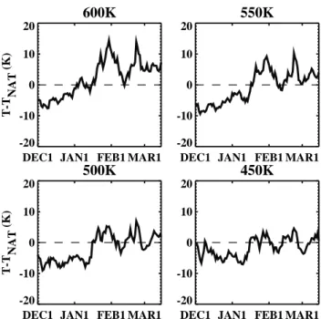
Fig. 1. Time series of T-Tnat in the Arctic vortex from 1
Decem-ber 2002 through 15 March 2003 for the 600 K, 550 K, 500 K, and 450 K potential temperature surfaces vortex wide. Temperatures are the minimum temperatures inside the polar vortex and were ob-tained from Met Office analyses. NAT condensation temperatures were computed using the Hanson and Mauersberger (1988) expres-sion, assuming 10 ppbv HNO3and 5 ppmv H2O.
chlorine activation, and understanding early winter ozone loss at high solar zenith angles. Although the early winter loss does not account for a large fraction of the total loss, Rex et al. (2002a, 2003) noted that a full understanding is required for reliable predictions of future ozone levels in the Arctic Stratosphere.
One of the complications in quantifying ozone loss is that no direct observations of chemical ozone loss rates exist. Rather, chemical loss rates must be inferred from the mea-surements with a priori knowledge of, or assumptions about, the ozone variations due to dynamical processes. As noted by Manney et al. (2003a), uncertainties in these dynamical processes are large and poorly quantified, and thus can lead to large uncertainties in the “measurements” of ozone loss. In order to determine the variation of ozone due solely to chemi-cal processes the dynamichemi-cal and chemichemi-cal variations must be separated in the observed ozone fields. Four methods have primarily been used to isolate photochemical loss (e.g., Har-ris et al., 2002; Rex et al., 2002b; Newman and Pyle, 2003):
1. The “Match” technique quantifies photochemical ozone loss by measuring the difference in ozone in an air par-cel sampled at different times (Rex et al., 2003, and references therein). “Matches” occur when trajectories indicate that the same air parcel is observed multiple times by one or more instruments (either ozone sondes
or satellites), within some prescribed tolerance limits. If the vortex is sampled homogeneously, the ozone loss result reflects vortex average conditions (Harris et al., 2002).
2. The “Tracer Correlation” technique removes the ef-fect of transport by comparing the pre-winter and post-winter relations between ozone volume mixing ratio and an inert tracer, such as nitrous oxide (N2O) or methane
(CH4), inside the vortex (Proffitt et al., 1990; M¨uller
et al., 1997, 2001). This method assumes that in the absence of ozone production or loss, the ozone/tracer relationship remains constant; thus, any post-winter de-viations from the pre-winter relationship are interpreted as chemically induced.
3. The “Vortex Average” technique quantifies dynamical variation for an average ozone profile inside the vortex by calculating vortex average descent rates from a ra-diative transfer model. This technique assumes that the dynamical contribution to ozone change inside the vor-tex is dominated by diabatic descent, and that mixing between vortex and extra-vortex air is minimal; there-fore, only vertical transport is considered (Hoppel et al., 2002).
4. The “Passive Subtraction” technique requires ozone to be simulated as a passive tracer. The passive ozone is then subtracted from ozone measurements to quantify the change in ozone due to chemistry (e.g., Manney et al., 1995a, 2003b). In this work we use a 3-D chemical transport model (CTM) to simulate ozone as a passive tracer (e.g., Goutail et al., 1997; Deniel et al., 1998; Hoppel et al., 2002) and will refer to this technique as the “CTM Passive Subtraction” (CTM-PS) technique. As mentioned by Guirlet et al. (2000) and Harris et al. (2002), quantitative comparisons of the different ozone loss calculations can be difficult since each method consid-ers different altitudes, time periods, and area averages of the vortex. When comparing ozone loss results it is critical to understand these differences as well as the weaknesses of each method. Two large sources of uncertainty in the Match method are errors in the trajectory calculations (Rex et al., 1999) and neglect of mixing. Many Match pairs are required in order to reduce errors sufficiently to produce statistically significant ozone loss estimates, and the Match technique as-sumes that the sampled air parcel does not mix with its sur-roundings along a trajectory. The Tracer Correlation tech-nique quantifies the variation of ozone due to transport using the correlation between ozone and an inert tracer. In order to define the tracer correlations adequately, data is needed throughout the stratosphere. Since ozone tracer correlations are often different outside the vortex than inside, processes such as descent and horizontal mixing can alter the correla-tions in ways that can mimic ozone loss (Michelsen et al.,
02 Dec 2002 22 Dec 2002 09 Jan 2003 21 Jan 2003
05 Feb 2003 17 Feb 2003 13 Mar 2003 30 Mar 2003
1.5 1.8 2.1 2.3 2.6 2.9 3.2 3.5 3.7 4.0 4.3 4.6 4.8 5.1 5.4 PV
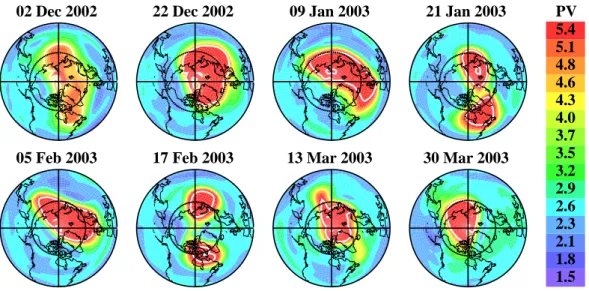
Fig. 2. Met Office PV (10−5Km2kg−1s−1)at the 500 K potential temperature surface for specific dates during the 2002–2003 winter from 90◦N to 30◦N. The inner vortex boundary is denoted by the solid white contour. The black dotted circle indicates the POAM measurement latitudes.
1998). Mixing across the vortex edge or differential descent and mixing within the vortex may disrupt the compactness of ozone/tracer relationships and can result in anomalous rela-tionships; such effects must be considered before estimates of ozone loss can be made reliably from tracer relationships (Plumb et al., 2000; Ray et al., 2002). The Vortex Aver-age method as applied by Hoppel et al. (2002) uses vortex-averaged descent rates, tantamount to assuming uniform de-scent within the vortex, and does not account for lateral mix-ing across the vortex edge. Lateral mixmix-ing across the vortex edge is particularly important to consider in winters when the vortex is disturbed. The CTM-PS technique includes hori-zontal transport, but it also has several areas of uncertainty. Most importantly, it is dependent on the proper initialization of the CTM ozone fields, correct representation of transport in the model, and proper gas phase chemistry to isolate het-erogeneous induced ozone loss.
The main purpose of this paper is to describe CTM-PS ozone loss results for the Arctic 2002–2003 winter using observations from the third Polar Ozone and Aerosol Mea-surement (POAM) instrument (Lucke et al., 1999) and the SLIMCAT CTM (Chipperfield, 1999). Comparisons be-tween CTM-PS results and Vortex Average results are also shown, but detailed analysis of these comparisons, as well as comparisons with the Match and Tracer Correlation ozone loss calculations, are the subject of future work. The CTM-PS technique, depending on the sophistication and accuracy of the CTM, is in some sense the most complete method for determining ozone loss. That is, if the chemistry and dynam-ics are accurate within the CTM, all the processes needed to deduce chemical ozone loss are included and few assump-tions are required. The CTM-PS technique is an integral part of the development of coupled Chemistry Climate Models
(CCMs), the framework of which relies on accurate treatment of ozone loss processes in the chemical calculations used. In-vestigations such as those described below will thus result in a more accurate investigation of the coupling between global climate change and polar ozone loss.
2 2002–2003 meteorology
The 2002–2003 winter can be characterized as an unusually cold early winter and dynamically active and warm mid to late winter (Manney et al., 2005). Figure 1 shows the mini-mum Met Office temperatures inside the Arctic polar vortex with respect to Nitric Acid Trihydrate (NAT) condensation temperatures (TNAT)at four different potential temperature levels from 450 K (about 18 km) to 600 K (about 22 km). TNAT values were computed using the expression given by Hanson and Mauersberger (1988), Met Office pressure, and by assuming 10 ppbv HNO3and 5 ppmv H2O. Vortex wide, minimum temperatures were below TNATuntil mid-January, with a few exceptions at 600 K. Throughout the lower strato-sphere temperatures increased rapidly in late January, as a major stratospheric warming occurred. Temperatures were just recovering toward pre-warming levels when a strong mi-nor warming occurred in February. Although temperatures began to decrease after the warming, the vortex was never again as cold as in December. After early February, mini-mum vortex temperatures reached TNATor fell below TNAT on a few occasions at 600 and 550 K. At 500 and 450 K vor-tex wide minima fell below TNATafter February.
Although the polar vortex was very cold in December and January, it was neither circular nor centered on the pole. Fig-ure 2 shows maps of the Met Office PV fields on the 500 K
POAM Measurement Locations
DEC1 JAN1 FEB1 MAR1 APR1 20 30 40 50 60 70 80 90 [Equivalent] Latitude
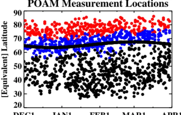
Fig. 3. Northern Hemisphere equivalent latitudes (dots) and
ge-ographic latitudes (solid curve) of POAM measurements on the 500 K potential temperature surface. Red indicates measurements taken within the inner edge of the vortex boundary, blue indicates measurements between the outer and inner edges, and black denotes all measurements taken beyond the outer edge.
potential temperature surface for specific days during the 2002–2003 winter. In December and January the vortex was often elongated, allowing air within it to make frequent ex-cursions into the sunlight at lower latitudes. As described below, the very low temperatures and prolonged solar expo-sure led to ozone loss as early as late December. However, the major warming in January followed by the strong minor warming in February caused the vortex to shrink and split, as indicated by the maps for 21 January and 17 February. The series of warming events also caused temperatures to in-crease, limiting the total amount of ozone loss over the winter (Manney et al., 2005).
3 POAM III observations in 2002–2003
POAM III (Lucke et al., 1999) is a nine-channel solar oc-cultation photometer with wavelength channels ranging from 0.353 to 1.02 µm to measure profiles of ozone, nitrogen diox-ide, water vapor, and aerosol extinction. During one day POAM makes 14–15 measurements around a circle of lati-tude in each hemisphere, with successive measurements sep-arated in longitude by about 25◦. The POAM measurement latitude varies smoothly and slowly over the course of a year between 55◦N and 73◦N in the northern hemisphere (NH) and between 63◦S and 88◦S in the southern hemisphere (SH). The POAM measurement latitude variation over the NH winter (the measurement coverage is the same each year) is shown in Fig. 3. Also shown in Fig. 3 is the equivalent lat-itude (Butchart and Remsberg, 1986) (equivalent latlat-itude is the latitude that would enclose the same area between it and the pole as does the PV contour) at 500 K of each POAM measurement obtained during the 2002–2003 winter. The PV fields used in the equivalent latitude calculation were ob-tained using the Met Office meteorological analysis. In this figure the measurements are color-coded according to their
position with respect to the vortex (outside: outside the outer edge, edge: between the inner and outer edge, and inside: inside the inner edge), which is defined using the discrimi-nation algorithm of Nash et al. (1996) and, as for the equiva-lent latitudes, the Met Office-derived PV. Figure 3 shows that although only a relatively narrow range of latitudes is sam-pled by POAM, a much larger range of equivalent latitudes was sampled during the 2002–2003 winter because the vor-tex was often elongated and displaced from the pole. Thus, POAM sampled inside, outside, and on the edge of the vortex on a nearly daily basis throughout the winter.
The POAM ozone data set used in this study is version 3.0 (Lumpe et al., 2002). Version 4.0 POAM data became available after the analysis for this work had been completed. Comparisons between version 3.0 and version 4.0 POAM ozone data indicate differences of less than 1% on average, so the results presented here are not expected to change sig-nificantly with the new version. The vertical resolution of the version 3.0 retrievals is approximately 1 km in the strato-sphere, and the random error is <10% above 10 km (<5% above 15 km) (Lumpe et al., 2002). This data set has un-dergone extensive validation and intercomparison with other remote sensing data sets and balloon-borne ozonesondes (Lumpe et al., 2003; Randall et al., 2003; Prados et al., 2003). Randall et al. (2003) show that on average, NH POAM ozone profiles agree to within about 5% with ozonesonde and other satellite data from 13 to 60 km. Below 13 km the POAM measurements appear to be biased increasingly high with de-creasing altitude reaching values of about 40% (0.1 ppmv) higher then ozonesondes at 10 km (Randall et al., 2003; Pra-dos et al., 2003).
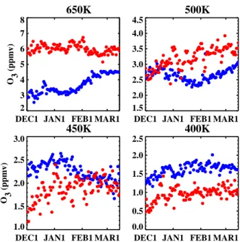
Figure 4 shows the evolution of ozone measured by POAM throughout the 2002–2003 winter from 400 K (about 15 km) to 650 K (about 25 km). The measurements are color-coded according to their position with respect to the vortex edge. Lower stratospheric ozone in the polar region generally in-creases throughout the winter due to descent of ozone-rich air from higher altitudes. At 650 K ozone outside the outer edge of the vortex is significantly higher than ozone inside the inner edge of the vortex primarily because poleward trans-port of ozone rich tropical and subtropical air is limited to the vortex exterior (e.g., Manney et al., 1995a; Randall et al., 1995). Enhanced diabatic descent causes an overall in-crease in vortex ozone, from about 3 ppmv in December to 4.5 ppmv in March. At 500 K vortex and extra-vortex ozone are nearly identical in early December. This is be-cause enhanced diabatic descent increases 500 K ozone mix-ing ratios sampled by POAM inside the vortex by about the same amount that mixing with subtropical extra-vortex air increases 500 K mixing ratios sampled by POAM outside the vortex. However, from late December to late January vor-tex ozone diverges from extra-vorvor-tex ozone, declining from about 3 ppmv to 2.3 ppmv. A gradual increase is then ob-served during February and March inside the vortex. At 400 and 450 K, enhanced diabatic descent causes vortex ozone to
exceed extra-vortex ozone in early December. At 450 K in late January, however, vortex ozone declines to values com-parable to those observed outside the vortex. We interpret the ozone declines at 500 and 450 K as evidence of chemical ozone loss. This interpretation is consistent with the meteo-rology of the 2002–2003 winter described in Sect. 2. Vortex air was cold enough in the early winter to support PSC for-mation, and had experienced significant solar exposure as it was drawn to lower latitudes. Further evidence that condi-tions were primed for ozone loss is seen in the POAM mea-surements of PSCs (not shown). In December of 2002 the proportion of POAM observations in which a PSC was de-tected was larger than previously observed in December by either POAM III or its predecessor, POAM II, which oper-ated from October 1993 to November 1996 (Alfred et al., 20051). PSC occurrence frequencies decreased substantially after the January 17 warming, with only sporadic observa-tions of PSCs in February and March.
4 SLIMCAT 3-D CTM
Here we summarize the main details of the SLIMCAT 3-D CTM and describe the initialization that was performed specifically for the study of the 2002–2003 Arctic winter. 4.1 Model description
SLIMCAT is a 3-D off-line chemical transport model de-scribed in Chipperfield (1999). The model has a detailed treatment of stratospheric chemistry, which includes all of the species believed to be important in the chemistry of the polar stratosphere, and a description of heterogeneous chem-istry on solid and liquid aerosols. The model temperatures and horizontal winds are specified from analyses and the ver-tical transport in the stratosphere is diagnosed from radiative heating rates. Radiative heating rates are used because they provide the best simulation of stratospheric transport. SLIM-CAT uses the Prather (1986) advection scheme which has very low numerical diffusion. In the stratosphere the model uses an isentropic coordinate and this has recently been ex-tended down to the surface using hybrid sigma-theta levels.
The setup of the model runs for the winter 2002–2003 sim-ulations used here is described in detail in Feng et al. (2005). They summarize recent changes in the model to improve the treatment of chemistry and transport relevant to the high latitude lower stratosphere aimed at improving the model performance. For the runs used here SLIMCAT was ini-tialized on 1 January 1989 and integrated at low horizontal resolution (7.5×7.5◦) for ∼14 years using European Centre
for Medium-Range Weather Forecasts (ECMWF) analyses 1Alfred, G., Bevilaqua, R. M., Fromm, M. D., et al.:
Observa-tions and analysis of polar stratospheric clouds detected by POAM III and SAGE III during the 2002/2003 northern hemisphere winter, Atmos. Chem. Phys. Discuss., in preparation, 2005.
650K
DEC1 JAN1 FEB1 MAR1 2 3 4 5 6 7 8 O 3 (ppmv)
500K
DEC1 JAN1 FEB1 MAR1 1.5 2.0 2.5 3.0 3.5 4.0 4.5
450K
DEC1 JAN1 FEB1 MAR1 1.0 1.5 2.0 2.5 3.0 O 3 (ppmv)
400K
DEC1 JAN1 FEB1 MAR1 0.0 0.5 1.0 1.5 2.0 2.5
Fig. 4. 2002/2003 POAM daily average observations on the 650 K,
500 K, 450 K, and 400 K potential temperature surfaces inside the inner vortex edge (blue) and outside the outer vortex edge (red).
(Feng et al., 2005). The model has 24 levels from the sur-face to ∼55 km and the resolution in the lower stratosphere is ∼2 km. Output from this low resolution run was inter-polated to a higher horizontal resolution (2.8×2.8◦) in mid-November 2002. This model was then integrated through the 2002–2003 Arctic winter in a series of experiments.
4.2 Ozone initialization
A large source of uncertainty in the CTM-PS method is errors in the CTM initialization, thus special attention was paid to the initial model ozone field. Satellite observations of ozone were used to reinitialize the SLIMCAT ozone fields (both the chemically integrated and passive fields) on 1 Decem-ber 2002. Only the ozone model fields were reinitialized in the model because of the lack of global observations of other constituents. There is thus the potential for inconsistencies in runs when ozone is not treated as a passive tracer, because the other constituents were determined from the multiannual run as described above. This needs to be considered when inter-preting the model and measurement differences; however, we still feel that it is better to use the ozone fields to constrain the model. The ozone fields were constructed from 2002 North-ern Hemisphere observations from POAM and the Halogen Occultation Experiment (HALOE) using PV-mapping, as de-scribed in Randall et al. (2002, 2005). For the 1 December initialization date, the ozone reconstruction included data ac-quired between 21 November and 11 December. Based on statistical analyses of a year of reconstructions (not shown), on average the ozone reconstructions agree with the satellite
0
2
4
6
8
400
600
800
1000
20021130-2 -1
0
1
2
400
600
800
1000
-40 -20 0
20 40
400
600
800
1000
Ozone (ppmv) Proxy-POAM (ppmv) (Proxy-POAM)/POAM (%)
0
2
4
6
8
400
600
800
1000
Potential Temperature (K)
20021201-2 -1
0
1
2
400
600
800
1000
-40 -20 0
20 40
400
600
800
1000
Ozone (ppmv) Proxy-POAM (ppmv) (Proxy-POAM)/POAM (%)
0
2
4
6
8
400
600
800
1000
20021202-2 -1
0
1
2
400
600
800
1000
-40 -20 0
20 40
400
600
800
1000
Ozone (ppmv) Proxy-POAM (ppmv) (Proxy-POAM)/POAM (%)
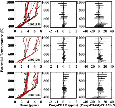
Fig. 5. Comparison of the ozone initialization profiles interpolated to the POAM measurement locations for 30 November (top row), 1
December (middle row), and 2 December (bottom row). The left column shows the 1 December initialization profiles (red) interpolated to the POAM measurement locations (black) on the dates shown. Average differences between the profiles are shown in ppmv (middle column) and percent (right column). Error bars denote 1σ standard deviation of the distribution.
data comprising them to within 1% above about 1000 K, but exhibit a 5% (0.1 ppmv) positive bias below 800 K. Figure 5 shows the POAM ozone profiles from 30 November through 2 December as well as the 1 December mapped initializa-tion fields interpolated to the POAM measurement locainitializa-tions on these dates (30 November and 2 December are shown be-cause POAM only made four measurements on 1 Decem-ber). The initialization fields overall compare well with the POAM observations, but are higher than the POAM obser-vations at 500 K. When combining satellite data and model results to infer ozone loss, it is critical that the model faith-fully represent the satellite data prior to any ozone loss. If there is an offset between the model ozone and satellite data, ozone loss (or production) will be inferred even on the ini-tial date of calculations. Such an iniini-tialization error will be carried through the calculations, affecting modeled ozone changes due to both horizontal and vertical transport. The 500 K discrepancy shown in Fig. 5 will lead to an overes-timate in the modeled ozone increase due to descent even at lower potential temperature levels, and hence an overesti-mate in the chemical loss inferred by subtracting the modeled passive ozone from the POAM ozone. These differences are considered when results are interpreted.
4.3 Pure passive and pseudo passive runs
For this study each SLIMCAT run contained two ozone fields. In addition to the chemically integrated “Active” ozone, which is coupled to the heating rate calculation, the model contained a “Pure Passive” ozone tracer. The “Pure Passive” ozone tracer was advected using identical transport to the other chemical species but with no chemical change. The model results were then interpolated to the POAM mea-surement locations. Chemical ozone loss was calculated by subtracting the Pure Passive model ozone from the POAM measurements (“inferred” loss) or from the Active model ozone (“modeled” loss). Conventionally, both gas phase and heterogeneous chemistry are turned off in the passive model with the CTM-PS technique. One concern with this and other ozone loss methods (e.g., tracer correlations) is that passively transported ozone is not expected to be accu-rate if transported for periods longer than approximately one month (Manney et al., 1995a, b). The main source of strato-spheric ozone is from production in the middle stratosphere at low latitudes (Brasseur and Solomon, 1984). Manney et al. (1995b) noted that if air is passively advected for long periods of time, this low-latitude ozone source will not be
DEC1 JAN1 FEB1 MAR1 400 450 500 550 600 650 700 Potential Temperature (K) 1.2 1.5 1.8 2.1 2.4 2.7 3.1 3.4 3.7 4.0 4.3 O3 (ppmv)
DEC1 JAN1 FEB1 MAR1 400 450 500 550 600 650 700 1.2 1.5 1.8 2.1 2.4 2.7 3.1 3.4 3.7 4.0 4.3 O3 (ppmv)
DEC1 JAN1 FEB1 MAR1 400 450 500 550 600 650 700
DEC1 JAN1 FEB1 MAR1 400 450 500 550 600 650 700 -0.60 -0.54 -0.48 -0.42 -0.36 -0.30 -0.24 -0.18 -0.12 -0.06 0.00 O3 Difference (ppmv)
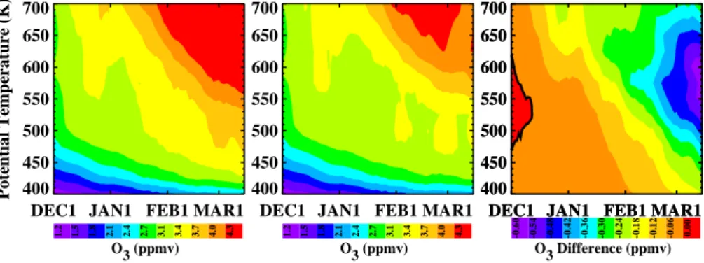
Fig. 6. Comparison of the SLIMCAT Passive ozone (ppmv) inside the vortex at the POAM measurement locations for the Pure Passive
(left) and Pseudo Passive (middle) runs, and for the difference between the two (right; Pseudo minus Pure). Ozone mixing ratios have been smoothed using a 7-day running average.
maintained. As a result, air passively transported poleward and downward may be deficient in ozone. On the other hand, at polar latitudes local NOx(NO+NO2)chemistry results in a net destruction of ozone in the middle stratosphere, so not accounting for this chemistry would result in the downward transport of too much ozone. Other ozone-destroying cat-alytic cycles can also be important in the lower and upper stratosphere (Lary, 1997). Thus, whether the net effect of gas phase chemistry is to increase or decrease ozone depends on a number of parameters that will vary in season, latitude, and altitude. For the December–March time period at high latitudes, photochemistry is expected to be important mainly above about 650 K (e.g. Garcia and Solomon, 1983; Randall et al., 1995), but these processes can also contribute appre-ciably at lower altitudes, as shown below. To explore the effects of gas phase chemistry on the ozone loss inferences, the model runs were first done with the conventional “Pure Passive” calculation, and then repeated with a “Pseudo Pas-sive” calculation, in which gas phase reactions remained ac-tivated, but cold, chlorine-activating heterogeneous chemical reactions on solid and liquid PSCs were switched off. Re-sults from both calculations are shown below to quantify the net change in ozone (production-loss, with the caveat that this could be influenced by errors in the transported ozone as described above) as well as the change due to heterogeneous processes alone.
Figure 6 compares model results inside the vortex at the POAM locations for the Pure Passive (no chemistry) and the Pseudo Passive (activated gas phase chemistry) runs. Dif-ferences between the Pseudo and Pure Passive ozone mix-ing ratios increase gradually in time at all altitudes, with the Pseudo Passive lower than the Pure Passive. Differences between the Pseudo Passive and Pure Passive reach about 0.6 ppmv in mid-March near 600 K. We attribute this to in-creasing catalytic ozone destruction as sunlight returns to the polar region. It is interesting that differences between the Pure and Pseudo Passive calculations decrease in magnitude above 600 K in late February and March. This results from
an increase in competition between catalytic ozone loss at high latitudes and production at lower latitudes (which was then followed by advection to high latitudes), so that the net effect of photochemistry is less significant. Differences are smaller at the lowest altitudes, consistent with the expecta-tion that photochemistry, either through direct or indirect (via descent of chemically processed air) mechanisms, should be less important at these altitudes. Nevertheless, Fig. 6 shows that even at potential temperatures as low as 450–500 K, gas phase chemistry, in the absence of chlorine-activating hetero-geneous reactions on solid and liquid PSCs, can contribute to ozone loss by as much as 0.4 ppmv by mid-March. It is also important to consider that there may be a potential incon-sistency in the Pseudo Passive, since only the ozone fields were reinitialized from observations. The Pure Passive ozone would not be affected since ozone is treated as a completely passive tracer. Additional analysis is required to determine the effect of the potential inconsistency.
5 Ozone loss during 2002–2003
In this section we apply the CTM-PS technique using both the Pure and Pseudo Passive SLIMCAT CTM results to infer the magnitude of ozone loss inside the Arctic vortex during the 2002–2003 winter from the POAM observations. CTM-PS results are then compared with those calculated using the Vortex Average technique.
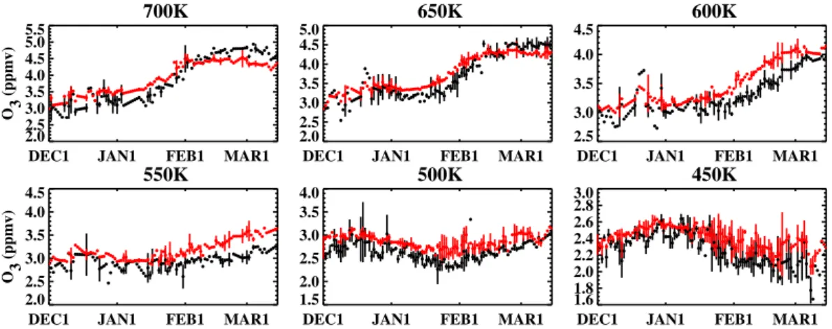
The Passive technique is illustrated in Fig. 7, which shows 2002–2003 time series of POAM ozone inside the vortex and the co-located passive modeled ozone at different potential temperatures. From 600 to 700 K (about 23 to 26 km), the overall character of the Pseudo Passive model and POAM time series in Fig. 7 is similar, showing generally increasing ozone mixing ratios throughout the winter. We attribute this overall increase to enhanced diabatic descent within the vor-tex. Agreement between the Pseudo Passive and POAM data is often within the error bars, although the model is system-atically higher than POAM in December and January by up
700K
DEC1 JAN1 FEB1 MAR1 2.0 2.5 3.0 3.5 4.0 4.5 5.0 5.5 O 3 (ppmv) 650K
DEC1 JAN1 FEB1 MAR1 2.0 2.5 3.0 3.5 4.0 4.5 5.0 600K
DEC1 JAN1 FEB1 MAR1 2.5 3.0 3.5 4.0 4.5 5.0 550K
DEC1 JAN1 FEB1 MAR1 2.0 2.5 3.0 3.5 4.0 4.5 O 3 (ppmv) 500K
DEC1 JAN1 FEB1 MAR1 1.5 2.0 2.5 3.0 3.5 4.0 4.5 450K
DEC1 JAN1 FEB1 MAR1 1.5 2.0 2.5 3.0 3.5 4.0
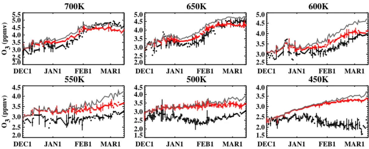
Fig. 7. Daily average ozone mixing ratios inside the vortex at the POAM measurement locations for POAM (black) and the SLIMCAT
Pseudo Passive (red) at the six indicated potential temperatures. Error bars denote 1σ standard deviation of the averages. Points without error bars indicate that only one POAM observation was made inside the vortex at a given potential temperature level. Chemical ozone loss is calculated by subtracting the Passive model from the POAM data. The Pure Passive is shown by the gray line, without error bars (which are approximately the same size as the error bars for the Pseudo Passive).
to 0.2 ppmv. Because this bias first appears within the first week in December, we attribute it to errors in the initializa-tion field that cannot be checked due to lack of global mea-surements. The necessity of including gas-phase chemistry in the Pseudo Passive model is apparent, as the agreement between the Pseudo Passive and POAM data is better than between the Pure Passive and POAM data throughout most of the winter. An exception to this occurs at 700 K in late February and March, when the Pseudo Passive model un-derestimates POAM ozone mixing ratios, whereas the Pure Passive is in agreement. Close inspection of the comparisons from 600–700 K indicates that in late February and March, ozone in the Pseudo Passive model systematically declines sooner than observed by POAM.
At 500 K, POAM measures increasing ozone in the first half of December, followed by decreasing ozone mixing ra-tios into late January, and then increasing ozone through mid-March. Model passive ozone at these altitudes steadily in-creases throughout the winter due to enhanced diabatic de-scent in the vortex. Initialization errors cause the Pseudo Passive model to exceed the POAM observations in early De-cember. From 2–6 December, for instance, the average dif-ference between the POAM data and Pseudo Passive model at 500 K is 0.31±0.11 ppmv. Nevertheless, it is clear that the decline starting in late December and continuing through January represents a divergence of the observations from the passive model that on average exceeds the initialization dif-ferences, an indication of chemical processes. Indeed, the average difference between the POAM data and Pseudo Pas-sive model at 500 K from 2–6 January is 0.63±0.10 ppmv, which is larger by a factor of 2 than the difference obtained at the beginning of December. That chemical loss started in late December and became increasingly statistically signif-icant with time suggests that the air parcels at 500 K
sam-pled by POAM at this time had been exposed to PSC for-mation temperatures and sunlight for prolonged periods of time. PSCs were observed by POAM between 650 K and 500 K from late November through mid January, with a few sightings in early February (Alfred et al., 20051). Trajec-tory calculations (not shown) confirm that air at the POAM measurement locations inside the vortex at 500 K in late De-cember had been exposed to temperatures below the NAT condensation temperature and to as much as 50 h of sunlight in the previous 10 days.
The 450 K ozone increase through mid-December in both the Pseudo Passive model and POAM observations is a sig-nature of enhanced diabatic descent inside the vortex and the absence of chemical loss. The observations begin to di-verge from the Pseudo Passive model in late December, as chemical ozone loss evidently begins, even though POAM ozone is still increasing. POAM ozone decreases by about 0.4 ppmv in January, but then remains relatively constant or declines slightly through mid-March, perhaps and indication of diabatic descent of air from above that has experienced heterogeneous loss. Very low ozone (<2 ppmv) is observed on several occasions in early March, at a time when PSCs were observed at the POAM measurement locations. It is thus possible that heterogeneous processing led to localized ozone loss. More analysis is required to determine if hetero-geneous processing caused the localized ozone loss on such a short time scale.
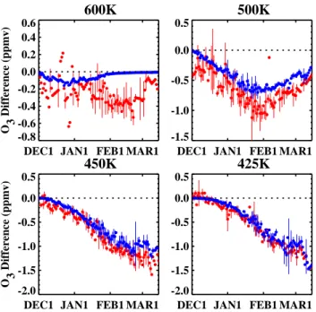
Chemical ozone loss inside the vortex inferred from the POAM observations in 2002–2003 is depicted as differences between the observations and the Passive models in Figs. 8 and 9, where negative differences signify loss. These fig-ures show results from both the Pure Passive and Pseudo Pas-sive calculations. There is little difference between the two model calculations in December at any potential temperature
700K
DEC1 JAN1 FEB1 MAR1 -1.0 -0.5 0.0 0.5 1.0 O3 Difference (ppmv) 650K
DEC1 JAN1 FEB1 MAR1 -1.0 -0.5 0.0 0.5 1.0 600K
DEC1 JAN1 FEB1 MAR1 -1.0 -0.5 0.0 0.5 1.0 550K
DEC1 JAN1 FEB1 MAR1 -1.5 -1.0 -0.5 0.0 0.5 O3 Difference (ppmv) 500K
DEC1 JAN1 FEB1 MAR1 -1.5 -1.0 -0.5 0.0 0.5 450K
DEC1 JAN1 FEB1 MAR1 -2.0 -1.5 -1.0 -0.5 0.0 0.5
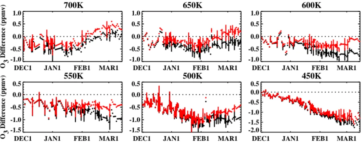
Fig. 8. Time series of the inferred ozone loss in 2002–2003 using the SLIMCAT Pure Passive (black) and Pseudo Passive (red) (see text
for details). Points represent daily averages of measurements inside the vortex. The dotted black line denotes 0 ppmv. Error bars denote 1σ standard deviation of the differences. Points without error bars indicate that only one POAM observation was made inside the vortex at a given potential temperature level.
DEC1 JAN1 FEB1 MAR1 400 450 500 550 600 650 700 Potential Temperature (K)
DEC1 JAN1 FEB1 MAR1 400 450 500 550 600 650 700 Potential Temperature (K) -1.5 -1.3 -1.1 -1.0 -0.8 -0.6 -0.4 -0.2 -0.1 0.1 0.3 O3 Difference (ppmv)
DEC1 JAN1 FEB1 MAR1 400 450 500 550 600 650 700
DEC1 JAN1 FEB1 MAR1 400 450 500 550 600 650 700 -1.5 -1.3 -1.1 -1.0 -0.8 -0.6 -0.4 -0.2 -0.1 0.1 0.3 O3 Difference (ppmv)
DEC1 JAN1 FEB1 MAR1 400 450 500 550 600 650 700 -1.5 -1.3 -1.1 -1.0 -0.8 -0.6 -0.4 -0.2 -0.1 0.1 0.3 O3 Difference (ppmv)
Fig. 9. Inferred ozone loss (ppmv) in 2002–2003, as represented by the difference between POAM and the SLIMCAT Pure Passive (left)
or Pseudo Passive (middle). The solid black line denotes the zero contour. Loss inferred from the POAM measurements using the vortex average technique initialized with the inferred 1 January Pure Passive loss profile is shown in the right panel. Data have been smoothed using a 7-day running average.
shown here. In both calculations, ozone loss (compared to the initial differences on 1 December) begins in late Decem-ber from about 450 to 550 K. Loss this early in the winter is unusual, and as noted above, occurred after cold vortex air was drawn equator ward to sunlit latitudes. After the ma-jor stratospheric warming on 17 January, ozone loss at 500 K ceases and begins to recover due to diabatic descent, how-ever, ozone loss continues at 450 K. Despite the January and February warming events vortex temperatures at 450 K still fell below TNAT as (shown in Fig. 1), consequently ozone loss persisted. The region of maximum loss gradually de-scends in altitude from about 500–550 K in late December to 400–450 K in mid March. Because of initialization er-rors, the difference plots are somewhat misleading, indicat-ing more ozone loss than would otherwise be inferred had the initialization been more accurate. Even at 425 K, where the initialization error is insignificant, an overestimate in the loss would result from propagation of errors as the air from higher
altitudes that contained an initial bias descends. We conser-vatively estimate this calculated loss bias to be on the order of 0.3 ppmv. Thus, Fig. 9 shows that by mid-March the max-imum ozone loss due to halogen-catalyzed ozone destruction after heterogeneous processing occurred near 425 K at a (cor-rected) value of approximately 1.2 ppmv. Gas phase chem-istry occurring in the absence of heterogeneous processing contributed an additional 0.4 ppmv of loss from 400–500 K. 5.1 Vortex average inferred ozone loss
Ozone loss inferred using the CTM-PS approach is now com-pared to that calculated using the vortex average technique (see Hoppel et al., 2002) applied to POAM observations in-side the vortex (Fig. 9, right panel). Heating rates from the radiative transfer model of Rosenfield et al. (1994) are used to calculate vortex averaged diabatic descent as a function of potential temperature. These descent rates are then used to
DEC1 JAN1 FEB1 MAR1 400 450 500 550 600 650 700 Potential Temperature (K)
DEC1 JAN1 FEB1 MAR1 400 450 500 550 600 650 700 Potential Temperature (K) -1.5 -1.3 -1.1 -1.0 -0.8 -0.6 -0.4 -0.2 -0.1 0.1 0.3 O3 Difference (ppmv)
DEC1 JAN1 FEB1 MAR1 400 450 500 550 600 650 700 1.2 1.5 1.8 2.1 2.4 2.7 3.1 3.4 3.7 4.0 4.3 O3 (ppmv)
DEC1 JAN1 FEB1 MAR1 400 450 500 550 600 650 700 1.2 1.5 1.8 2.1 2.4 2.7 3.1 3.4 3.7 4.0 4.3 O3 (ppmv)
Fig. 10. 2002/2003 CTM-PS modeled ozone difference (ppmv) at the POAM measurement locations inside the vortex (left), calculated as
the Active model ozone (middle) minus the Pseudo Passive model ozone (see Fig. 7). Negative values indicate modeled ozone loss. For comparison, the POAM ozone observations (ppmv) are shown in the right panel. Solid black lines in the left panel denote 0 differences. Ozone mixing ratios have been smoothed using a 7-day running average.
600K
DEC1 JAN1 FEB1 MAR1 -0.8 -0.6 -0.4 -0.2 0.0 0.2 0.4 0.6 O 3 Difference (ppmv) 500K
DEC1 JAN1 FEB1 MAR1 -1.5 -1.0 -0.5 0.0 0.5 450K
DEC1 JAN1 FEB1 MAR1 -2.0 -1.5 -1.0 -0.5 0.0 0.5 O 3 Difference (ppmv) 425K
DEC1 JAN1 FEB1 MAR1 -2.0 -1.5 -1.0 -0.5 0.0 0.5
Fig. 11. Comparison of the modeled ozone loss inside the vortex
(blue) to the inferred ozone loss using the Pseudo Passive (red). Error bars denote 1σ standard deviation of the average differences. Points without error bars indicate that only one POAM observation was made inside the vortex at a given potential temperature level.
estimate the vortex average ozone variation due to dynam-ics. Since the vortex average technique shows loss due to all chemical processes, it should only be compared to the Pure Passive CTM-PS result. The vortex average calculation does not start until 1 January, in order to minimize the errors due to cross-vortex mixing while still capturing the start of signif-icant ozone loss. To account for the later initialization date, the 1 January loss calculated by the Pure Passive CTM-PS approach was added to the initialization of the vortex aver-age calculation.
The vortex average loss is similar to the CTM-PS re-sults. The region of maximum ozone loss descends gradu-ally throughout the winter in the lower stratosphere, and is located at approximately the same theta level as in the CTM-PS inference. However, more ozone loss occurs in the vortex average calculation near 400 K than in the CTM-PS calcula-tion. A likely explanation is horizontal transport or mixing across the vortex edge, which is not included in the vortex average approach (Hoppel et al., 2002). During highly dis-turbed winters, this can be a large source of error in the vor-tex average calculation. At 400 K, the Northern Hemisphere vortex is never very impermeable at these lower potential lev-els (Manney et al., 1994) and any mixing with extra-vortex air will decrease ozone mixing ratios inside the vortex. By omitting this effect the vortex average method will overes-timate the ozone loss (the dynamical component subtracted from the observations will be too high, so the difference will be too large). Just the opposite will occur above 500 K, where extra-vortex ozone mixing ratios are larger than those inside the vortex. Whether this effect was large enough in 2002– 2003 to cause the discrepancies shown in Fig. 9 is a subject of future investigation.
5.2 CTM-PS modeled ozone loss
In this section we compare the inferred ozone loss to the SLIMCAT modeled loss using the Active and Pseudo Passive ozone fields. SLIMCAT modeled ozone loss inside the vor-tex is shown in Fig. 10, and is compared to the inferred loss in Fig. 11. Similar to the inferred loss, the region of maximum modeled loss descends from about 500–550 K in late Decem-ber to 425–450 K by mid-March as shown in Fig. 11. The magnitude of the modeled loss in mid-March at 450 K and 500 K is about 0.2–0.3 ppmv less than that inferred from the observations. This is consistent with the initialization error in the inferred loss calculations discussed above. Similar to the inferred loss calculation, the maximum modeled loss oc-curs at 425 K. Additionally, the magnitude of the maximum
700K
DEC1 JAN1 FEB1 MAR1 2.0 2.5 3.0 3.5 4.0 4.5 5.0 5.5 O3 (ppmv) 650K
DEC1 JAN1 FEB1 MAR1 2.0 2.5 3.0 3.5 4.0 4.5 5.0 600K
DEC1 JAN1 FEB1 MAR1 2.5 3.0 3.5 4.0 4.5 550K
DEC1 JAN1 FEB1 MAR1 2.0 2.5 3.0 3.5 4.0 4.5 O3 (ppmv) 500K
DEC1 JAN1 FEB1 MAR1 1.5 2.0 2.5 3.0 3.5 4.0 450K
DEC1 JAN1 FEB1 MAR1 1.6 1.8 2.0 2.2 2.4 2.6 2.8 3.0
Fig. 12. 2002/2003 POAM (black) and SLIMCAT Active (red) In-V daily average ozone mixing ratios at the potential temperatures indicated
in each panel. “Error” bars represent the standard deviation of the distribution of measurements/model on each day.
modeled loss is approximately 1.2 ppmv by 15 March. These results suggest that SLIMCAT reliably simulates the obser-vations of ozone during 2002–2003. This is shown clearly in the two right panels of Fig. 10 and in Fig. 12, which show contour plots and time series, respectively, of the POAM measurements and the Active model ozone. At 450 K, the model and observations generally agree within the standard deviations of the data, with a small systematic bias between the two that is largely due to initialization errors. There is an indication that the model might underestimate the loss at 450 K in March, but variations in the distributions are too large to ascribe quantitative significance to this. At 500 K and 600 K, the modeled ozone loss and inferred ozone loss start to diverge in late January, with SLIMCAT underesti-mating ozone loss at both levels. The disagreement is man-ifested as a failure of the model to maintain ozone loss as long as is observed, which as shown in Fig. 12 is caused by an overestimate of ozone at these levels by the model. This may indicate that the model incorrectly simulates the effects of the late January major warming at these levels, allowing too much mixing with extra-vortex air or too much diabatic descent inside the vortex. However, above 600 K in February and March model ozone is too low, possibly suggesting an underestimate of descent rates or an underestimate of mix-ing.
6 Summary
We have presented an overview of the 2002–2003 Arctic ozone loss results computed from the POAM satellite obser-vations and the SLIMCAT CTM using the CTM-PS tech-nique. PSC occurrences peaked in December when the 2002–2003 stratospheric temperatures were at their lowest. Dynamical activity led to stretching of the vortex to lower latitudes, which increased the amount of solar exposure re-ceived by the vortex early in the winter, leading to a late
De-cember onset of ozone loss. Stratospheric warming events limited PSC formation in late winter and early spring. As a result, the maximum ozone loss inferred from POAM data for the 2002–2003 winter was moderate compared to other cold Arctic winters in the late-1990s.
Ozone loss results inferred from POAM observations and a Pseudo Passive (activated gas phase chemistry) model were compared with those from a Pure Passive (no chemistry) model to determine the influence of gas phase chemistry on CTM-PS ozone loss calculations. The largest differences in the two passive fields occurred above 450 K at a value of .6 ppmv and can be attributed to NOxchemistry included in the Pseudo Passive run. After accounting for initialization errors, the maximum ozone loss inferred from POAM obser-vations and both CTM-PS calculations was approximately 1.2 ppmv by mid March between 450 and 425 K.
The CTM-PS calculations were compared to Vortex Av-erage ozone loss calculations. Ozone loss from the Vortex Average technique was similar to the CTM-PS technique, ex-cept that more loss was inferred near 400 K and less loss was inferred at 500 K. Additional work is required to understand the differences between the two techniques.
The SLIMCAT model was also run with the full chemistry in order to compare model ozone loss with inferred ozone loss from the POAM observations. Earlier studies have shown CTMs have had difficulty reproducing the extent of denitrification and chlorine activation observed during cold Arctic winters and, as a result, CTMs have typically under-estimated ozone loss under these conditions. Recent changes made in SLIMCAT, as discussed in Feng et al. (2005), have improved the model’s ability to reproduce polar dynamical and chemical processes. Consequently, the SLIMCAT model produces similar ozone loss morphology to the in-ferred results for the 2002–2003 winter, with loss occurring in late December near 550 K and descending throughout the winter, maximizing near 425 K by 15 March at around 1.2 ppmv. SLIMCAT’s ability to simulate ozone loss in Arctic winters with different meteorological conditions will
be the subject of future work. Initialization remains an issue for the CTM-PS technique. Future near global observations from NASA’s Earth Observing System Aura spacecraft will be used to initialize CTM fields and to calculate ozone loss with the CTM-PS technique, resulting in improved inferred and modeled ozone loss calculations.
Edited by: K. Carslaw
References
Becker, G., M¨uller, R., McKenna, D. S., Rex, M., Carslaw, K., and Oelhaf, H.: Ozone loss rates in the Arctic stratosphere in the winter 1994–1995: Model simulations underestimate results of the Match analysis, J. Geophys. Res., 105, 15 175–15 184, 2000. Butchart, N. and Remsberg, E. E.: The area of the stratospheric polar vortex as a diagnostic for tracer tracer transport on an isen-tropic surface, J. Atmos. Sci., 43, 1319–1339, 1986.
Chipperfield, M. P.: Multiannual simulations with a three-dimensional chemical transport model, J. Geophys. Res., 104, 1781–1805, 1999.
Chipperfield, M. P., Lee, A. M., and Pyle, J. A.: Model calcula-tions of ozone depletion in the Arctic polar vortex for 1991/92 to 1994/95, Geophys. Res. Lett., 23, 559–562, 1996.
Deniel, C., Bevilaqua, R. M., Pommereau, J. P., and Lef`evre, F.: Arctic chemical ozone depletion during the 1994–1995 winter deduced from POAM II satellite observations and the REPROBUS three-dimensional model, J. Geophys. Res., 103, 19 231–19 244, 1998.
Feng, W., Chipperfield, M. P., Davies, S., Sen, B., Toon, G., Blavier, J. F., Webster, C. R., Volk, C. M., Ulanovsky, A., Ravegnani, F., von der Gathen, P., Jost, H., Richard, E. C., and Claude, H.: Three-Dimensional Model Study of the Arctic Ozone Loss in 2002/03 and Comparison with 1999/2000 and 2003/04, Atmos. Chem. Phys., 5, 139–152, 2005,
SRef-ID: 1680-7324/acp/2005-5-139.
Garcia, R. R. and Solomon, S.: A numerical model of the zonally averaged dynamical and chemical structure of the middle atmo-sphere, J. Geophys. Res., 88, 1379–1400, 1983.
Goutail, F., Harris, N. R. P., Kilbane-Dawe, I., and Amanatidis, G. T.: Ozone loss: the global picture, Proc. European Ozone Meet-ing, Schliersee, Germany, 1997.
Guirlet, M., Chipperfield, M. P., Pyle, J. A., Goutail, F., Pom-mereau, J. P., and Kyr¨o, E.: Modeled Arctic ozone depletion in winter 1997/1998 and comparison with previous winters, J. Geophys. Res., 105, 22 185–22 200, 2000.
Hanson, D. and Mauersberger, K.: Laboratory studies of the ni-tric acid trihydrate: Implications for the south polar stratosphere, Geophys. Res. Lett., 15, 855–858, 1988.
Harris, N. R. P., Rex, M., Goutail, F., Knudsen, B. M., Manney, G. L., M¨uller, R., and von der Gathen, P.: Comparison of empiri-cally derived ozone losses in the Arctic vortex, J. Geophys. Res., 107(D20), doi:10.1029/2001JD000482, 2002.
Hoppel, K., Bevilaqua, R. M., Nedoluha, G., Deniel, C., Lef`evre, F., Lumpe, J., Fromm, M., Randall, C. E., Rosen-field, J., and Rex, M.: POAMIII observations of arctic ozone loss for the 1999/2000 winter, J. Geophys. Res., 107(D20), doi:10.1029/2001JD000476, 2002.
Lucke, R. L., Korwan, D. R., Bevilaqua, R. M., Hornstein, J. S., Shettle, E. P., Chen, D. T., Daehler, M., Lumpe, J. D., Fromm, M. D., Debrestian, D., Neff, B., Squire, M., Koniq-Langlo, G., and Davies, J.: The polar ozone and aerosol measurement (POAM) III instrument and early validation results, J. Geophys. Res., 104, 18 785–18 799, 1999.
Lumpe, J. D., Bevilacqua, R. M., Hoppel, K. W., and Randall, C. E.: POAM III retrieval algorithm and error analysis, J. Geophys. Res., 107(D21), 4575, doi:10.1029/2002JD002137, 2002. Lumpe, J. D., Fromm, M., Hoppel, K., Bevilaqua, R. M., Randall,
C. E., Browell, E. V., Grant, W. B., McGee, T., Burris, J., Twigg, L., Richard, E. C., Toon, G. C., Margitan, J. J., Sen, B., Pfeil-sticker, K., Boesch, H., Fitzenberger, R., Goutail, F., and Pom-mereau, J.-P.: Comparison of POAM III ozone measurements with correlative aircraft and balloon data during SOLVE, J. Geo-phys. Res., 107, 8316, doi:10.1029/2001JD000472, 2003. Manney, G. L., Zurek, R. W., O’Neil, A., and Swinbank, R.: On the
motions of air through the stratosphere polar vortex, J. Atmos. Sci., 51, 2973–2994, 1994.
Manney, G. L., Zurek, R. W., Lahoz, W. A., Harwood, R. S., Kumer, J. B., Mergenthaler, J., Roche, A. E., O’Neill, A., Swin-bank, R., and Waters, J. W.: Lagrangian transport calculations using UARS data, Part II: Ozone, J. Atmos. Sci., 52, 3069–3081, 1995a.
Manney, G. L., Froidevaux, L., Waters, J. W., and Zurek, R. W.: Evolution of Microwave Limb Sounder ozone and the polar vor-tex during winter, J. Geophys. Res., 100, 2953–2972, 1995b. Manney, G. L., Froidevaux, L., Santee, M. L., Livesey, N. J.,
Sabutis, J. L., and Waters, J. W.: Variability of ozone loss dur-ing Arctic winter (1991–2000) estimated from UARS Microwave Limb Sounder measurements, J. Geophys. Res., 108(D4), 4149, doi:10.1029/2002JD002634, 2003a.
Manney, G. L., Sabutis, J. L., Pawson, S., Santee, M. L., Nau-jokat, B., Swinbank, R., Gelman, M. E., and Ebisuzaki, W.: Lower stratospheric temperature differences between meteoro-logical analyses in two cold Arctic winters and their impact on polar processing studies, J. Geophys. Res., 10-8(D5), 8328, doi:10.1029/2001JD001149, 2003b.
Manney, G. L., Kr¨uger, K., Sabutis, J. L., Sena, S. A., and Paw-son, S.: The remarkable 2003–2004 winter and other recent warm winters in the Arctic stratosphere since the late 1990s, J. Geophys. Res., 110(D4), D04107, doi:10.1029/2004JD005367, 2005.
Michelsen, H. A., Manney, G. L., Gunson, M. R., and Zander, R.: Correlations of stratospheric abundances of NOy, O3, N2O,
and CH4derived from ATMOS measurements, J. Geophys. Res.,
103, 28 347–28 359, 1998.
M¨uller, R., Crutzen, P. J., Grooß, J.-U., Br¨uhl, C., Russel III, J. M., Gernandt, H., McKenna, D. S., and Tuck, A. F.: Severe chemical ozone loss in the Arctic during the winter of 1995–1996, Nature, 389, 709–712, 1997.
M¨uller, R., Schmidt, U., Engel, A., McKenna, D. S., and Proffitt, M. H.: The O3/N2O relationship from balloon-borne observa-tions as a measure of Arctic ozone loss in 1991–1992, Q.N.R. Meteorol. Soc., 127, 1389–1412, 2001.
Nash, E. R., Newman, P. A., Rosenfield, J. E., and Schoeberl, M. R.: An objective determination of the polar vortex using Ertel’s potential vorticity, J. Geophys. Res., 101, 9471–9478, 1996.
Newman, P. A., Pyle, J. A. (Lead Authors), Austin, J., Braathen, G. O., Canziani, P. O., Carslaw, K. S., de F. Forster, P. M., Godin-Beekmann, S., Knudsen, B. M., Kreher, K., Nakane, H., Pawson, S., Ramaswamy, V., Rex, M., Salawitch, R. J., Shindell, D. T., Tabazadeh, A., and Toohey, D. W.: Polar Stratospheric Ozone: Past and Future, Chapter 3 in “Scientific Assessment of Ozone Depletion: 2002, Global Ozone Research and Monitoring Project – Report No. 47”, Geneva, 2003.
Pierce, R. B., Saadi, J. A., Fairlie, T. D., Natarajan, M., Harvey, V. L., Grose, W. L., Russell III, J. M., Bevilaqua, R., Eckermann, S. D., Fahey, D., Popp, P., Richard, E., Stimpfle, R., Toon, G. C., Webster, C. R., and Elkins, J.: Large-scale chemical evolution of the Arctic vortex during the 1999/2000 winter: HALOE/POAM III Lagrangian photochemical modeling for the SAGE III Ozone Loss and Validation Experiment (SOLVE) campaign, J. Geo-phys. Res., 108(D5), 8317, doi:10.1029/2001JD001063, 2003. Plumb, R. A., Waugh, D. W., and Chipperfield, M. P.: The effects of
mixing on tracer relationships in the polar vortices, J. Geophys. Res., 105, 10 047–10 062, 2000.
Prados, A. I., Nedoluha, G. E., Bevilacqua, R. M., Allen, D. R., Hoppel, K. W., and Marenco, A.: POAM III ozone in the up-per troposphere and lowermost stratosphere: Seasonal variabil-ity and comparisons to aircraft observations, J. Geophys. Res., 108(D7), 4218–4228, 2003.
Prather, M. J.: Numerical advection by conservation of second-order moments, J. Geophys. Res., 91, 6671–6681, 1986. Randall, C. E., Rusch, D. W., Bevilacqua, R. M., Lumpe, J.,
Ainsworth, T. L., Debrestian, D., Fromm, M., Krigman, S. S., Hornstein, J. S., Shettle, E. P., Olivero, J. J., and Clancy, R. T.: Preliminary results from POAM II: Stratospheric ozone at high northern latitudes, Geophys. Res. Lett., 22, 2733–2736, 1995. Randall, C. E., Lumpe, J. D., Bevilacqua, R. M., Hoppel, K.
W., Fromm, M. D., Salawitch, R. J., Swartz, W. H., Lloyd, S. A., Kyr¨o, E., von der Gathen, P., Claude, H., Davies, J., DeBacker, H., Dier, H., Molyneux, M. J., and Sancho, J.: Reconstruction of three-dimensional ozone fields using POAM III during the SOLVE, J. Geophys. Res., 107(D20), 8299, doi:10.1029/2001JD000471, 2002.
Randall, C. E., Rusch, D.W., Bevilaqua, R. M., Hoppel, K. W., Lumpe, J. D., Shettle, E., Thompson, E., Deaver, L., Zawodny, J., Kyr¨o, E., Johnson, B., Kelder, H., Dorokhov, V. M., K¨onig-Langlo, G., and Gil, M.: Validation of POAMIII ozone: Com-parisons with ozonesonde and satellite data, J. Geophys. Res., 108(D12), 4367, doi:10.1029/2002JD002944, 2003.
Randall, C. E., Manney, G. L., Allen, D. R., Bevilaqua, R. M., Hornstein, J., Trepte, C., Lahoz, W., Ajtic, J., and Bodeker, G.: Reconstruction and simulation of stratospheric ozone distribu-tions during the 2002 austral winter, J. Atmos. Sci., 62, 748–764, 2005.
Ray, E. A., Moore, F. L., Elkins, J. W., Hurst, D. F., Romashkin, P. A., Dutton, G. S., and Fahey, D. W.: Descent and mix-ing in the 1999–2000 northern polar vortex inferred from in situ tracer measurements, J. Geophys. Res., 107(D20), 8285, doi:10.1029/2001JD000961, 2002.
Rex, M., von der Gathen, P., Braathen, G. O., Harris, N. R. P., et al.: Chemical ozone loss in the Arctic winter 1994/1995 as de-termined by the Match technique, J. Atmos. Chem., 32, 35–39, 1999.
Rex, M., Toohey, D., and Harris, N. R. P.: Report on the Arc-tic Ozone Loss Workshop, SPARC (Stratospheric Processes and their Role in Climate) Newsletter 19, 26–29, 2002a.
Rex, M., Salawitch, R. J., Harris, N. R. P., von der Gathen, P., Braathen, G. O., Schulz, A., Deckelmann, H., Chipperfield, M., Sinnhuber, B.-M., Reimer, E., Alfier, R., Bevilacqua, R., Hop-pel, K., Fromm, M., Lumpe, J., K¨ullmann, H., Kleinb¨ohl, A., Bremer, H., von K¨onig, M., K¨unzi, K., Toohey, D., V¨omel, H., Richard, E., Aikin, K., Jost, H., Greenblatt, J. B., Loewen-stein, M., Podolske, J. R., Webster, C. R., Flesch, G. J., Scott, D. C., Herman, R. L., Elkins, J. W., Ray, E. A., Moore, F. L., Hurst, D. F., Romashkin, P., Toon, G. C., Sen, B., Margitan, J. J., Wennberg, P., Neuber, R., Allart, M., Bojkov, B. R., Claude, H., Davies, J., Davies, W., De Backer, H., Dier, H., Dorokhov, V., Fast, H., Kondo, Y., Kyr¨o, E., Litynska, Z., Mikkelsen, I. S., Molyneux, M. J., Moran, E., Nagai, T., Nakane, H., Parrondo, C., Ravegnani, F., Skrivankova, P., Viatte, P., and Yushkov, V.: Chemical depletion of Arctic ozone in winter 1999/2000, J. Geo-phys. Res., 107(D20), 8276, doi:10.1029/2001JD000533, 2002b. Rex, M., Salawitch, R. J., Santee, M. L., Waters, J. W., Hoppel, K., and Bevilaqua, R.: On the unexplained stratospheric ozone losses during cold Arctic Januaries, Geophys. Res. Lett., 30(1), 1008, doi:10.1029/2002GL016008, 2003.
Rosenfield, J. E., Newman, P. A., and Schoeberl, M. R.: Compu-tations of diabatic descent in the stratospheric polar vortex, J. Geophys. Res., 99, 16 677–16 689, 1994.