Spherical Radiative Transfer in C++ (SRTC++): A Parallel Monte Carlo Radiative Transfer Model for Titan

(1)

HAL Id: insu-02780332

https://hal-insu.archives-ouvertes.fr/insu-02780332

Submitted on 4 Jun 2020

HAL is a multi-disciplinary open access

archive for the deposit and dissemination of

sci-entific research documents, whether they are

pub-lished or not. The documents may come from

teaching and research institutions in France or

abroad, or from public or private research centers.

L’archive ouverte pluridisciplinaire HAL, est

destinée au dépôt et à la diffusion de documents

scientifiques de niveau recherche, publiés ou non,

émanant des établissements d’enseignement et de

recherche français ou étrangers, des laboratoires

publics ou privés.

Spherical Radiative Transfer in C++ (SRTC++): A

Parallel Monte Carlo Radiative Transfer Model for Titan

Jason Barnes, Shannon Mackenzie, Eliot Young, Laura Trouille, Sébastien

Rodriguez, Thomas Cornet, Brian Jackson, Máté Ádámkovics, Christophe

Sotin, Jason Soderblom

To cite this version:

Jason Barnes, Shannon Mackenzie, Eliot Young, Laura Trouille, Sébastien Rodriguez, et al..

Spher-ical Radiative Transfer in C++ (SRTC++): A Parallel Monte Carlo Radiative Transfer Model for

Titan. Astronomical Journal, American Astronomical Society, 2018, 155 (6), pp.264.

�10.3847/1538-3881/aac2db�. �insu-02780332�

(2)

Spherical Radiative Transfer in C

++ (SRTC++): A Parallel Monte Carlo Radiative

Transfer Model for Titan

Jason W. Barnes1 , Shannon M. MacKenzie1, Eliot F. Young2, Laura E. Trouille3, Sèbastien Rodriguez4, Thomas Cornet4, Brian K. Jackson5 , Máté Ádámkovics6, Christophe Sotin7, and Jason M. Soderblom8

1

Department of Physics; University of Idaho; Moscow, Idaho 83844-0903, USA;jwbarnes@uidaho.edu

2

Space Studies Department, Southwest Research Institute, Boulder, CO 80302, USA

3

Adler Planetarium, Chicago, IL 60605, USA

4

Institut de Physique du Globe de Paris(IPGP), CNRS-UMR 7154, Université Paris-Diderot, USPC, Paris, France

5

Department of Physics, Boise State University, Boise, Idaho 83725-1570, USA

6

Physics and Astronomy Department, Clemson University, Clemson, South Carolina 29634, USA

7

Jet Propulsion Laboratory, California Institute of Technology, Pasadena, CA 91109, USA

8

Earth, Atmospheric and Planetary Sciences, Massachusetts Institute of Technology, Cambridge, MA 02139, USA Received 2017 October 27; revised 2018 April 24; accepted 2018 May 3; published 2018 June 4

Abstract

We present a new computer program, SRTC++, to solve spatial problems associated with explorations of Saturn’s moon Titan. The program implements a three-dimensional structure well-suited to addressing shortcomings arising from plane-parallel radiative transfer approaches. SRTC++ʼs design uses parallel processing in an object-oriented, compiled computer language (C++) leading to a ﬂexible and fast architecture. We validate SRTC++ using analytical results, semianalytical radiative transfer expressions, and an existing Titan plane-parallel model. SRTC+ +complements existing approaches, addressing spatial problems like near-limb and near-terminator geometries, non-Lambertian surface phase functions(including specular reﬂections), and surface albedo nonuniformity. Key words: planets and satellites: individual(Titan) – radiative transfer

1. Introduction

Titan’s thick, extended, hazy atmosphere elicits complex interactions of incoming photons with aerosols, gases, and the surface. Scattering by haze aerosol particles smears visibility of Titan’s surface, particularly at short wavelengths where haze particles have large extinctions (Smith et al. 1981; Richardson et al. 2004; Porco et al. 2005; Tomasko & West

2010; Maltagliati et al. 2015a). Gaseous methane, nitrogen,

and carbon monoxide in Titan’s atmosphere absorb light at most near-infrared wavelengths, permitting transmission from the surface only within distinct spectral windows (Grifﬁth

1993; Smith et al.1996; Barnes et al.2007; Vixie et al.2012).

And Titan’s heterogeneous surface (Grifﬁth 1993; Barnes et al. 2005) exhibits spectral units with varying reﬂectance

phase functions, including specular reﬂections off the smooth liquid lakes and seas (Stephan et al.2010; Soderblom et al.

2012; Barnes et al.2013). We illustrate some of these effects

in Figure 1.

Given the complex geometry and processes involved, inversion of reﬂectance spectra to independently ascertain surface and atmospheric parameters has proven challenging. Currently working models for Titan typically assume a plane-parallel one-dimensional (1D) atmosphere (e.g., McKay et al.

1989; Rannou et al. 2003; Rodriguez et al. 2006; Grifﬁth et al. 2012a; Maltagliati et al. 2015b; but see also Xu et al.

2013, which uses a spherical-shell assumption instead of plane-parallel). And they do so for good reasons. Quality 1D algorithms exist and have been thoroughly tested, and 1D codes’ approximations allow for fast radiative transfer calculations, thus enabling their practical use for spectral modeling (Young et al. 2002; Hirtzig et al. 2013) and the inversion of surface

albedo(Coustenis et al.1995; Grifﬁth et al.2012a; Solomonidou et al. 2014; Maltagliati et al.2015b; Solomonidou et al. 2016; Ádámkovics et al.2016).

Some subsets of Titan problems do not lend themselves well to being solved using 1D plane-parallel codes, however. Titan’s extended atmosphere leads to a dramatic falloff in the accuracy of the 1D plane-parallel approximation beyond incidence and emission angles of ∼60° (with signiﬁcant deviations at geometries as low as ∼35°–40° incidence for an extended atmosphere like Titan’s). Hence, observations near Titan’s limb, or near its poles, cannot be modeled using existing algorithms without complex modiﬁcations. One-dimensional codes by their nature do not model spatial problems like the adjacency effect, simulations of spatial resolution capabilities, indirect illumination beyond the terminator, and non-Lambertian surface phase functions.

To solve this spatial class of Titan radiative transfer problems, we have written a new radiative transfer computer program. The new algorithm uses a Monte Carlo approach in conjunction with fully spherical atmospheric geometry so that it can be used at extreme geometries and to solve spatial problems. Although the new code tracks photons in parallel, its speed still leaves much to be desired relative to conventional 1D plane-parallel approaches (e.g., Grifﬁth et al. 2012b; Solomonidou et al. 2014). Hence, our new approach is

designed to complement, and not to supplant, the current generation of radiative transfer solvers.

Although our work resembles existing astrophysical Monte Carlo radiative transfer solvers, like Hyperion (Robi-taille 2011), SUNRISE (Jonsson 2006), MC3D (Wolf 2003),

and SKIRT(Baes et al.2003) in many aspects, our strengths lie

in our design based around planetary remote sensing problems. Although our approach is general and could in principle be adapted for other purposes, we assume a central spherical solid body and allow for multiple observation viewpoints as might be seen from spacecraft. Together, these design choices allow both easier problem setup and more rapid and efﬁcient computation of the results.

(3)

We call the new code SRTC++ for “Spherical Radiative Transfer in C++”. We describe the nuts and bolts of the code itself, including the treatment of atmospheric structure, the generation of input photons, the photons’ traverse through that atmosphere, and our detector implementation in Section2. We then validate our results by comparing to the results of plane-parallel radiative transfer models in Section 3. Benchmarking discussions proceed in Section 4. Finally, we conclude with discussion of future application of SRTC++ in Section 5.

2. Computation

Spherical Radiative Transfer in C++ (SRTC++) is based on an earlier algorithm, SRTC, which was written in Interactive Data Language (IDL) by two of us (EFY and LET) but never published. We make no assumptions about atmospheric structure or scattering qualities, but rather virtually throw photons toward the target and probabilistically calculate their behavior. We ﬁrst calculate where the photon experiences a scattering event, which we determine randomly ﬁrst in optical depth space and later in physical space. At each of these randomly determined scattering events, we update the detector to record the visible response corresponding to the scatter. Then we probabilistically calculate a new direction for the photon post-scatter from the scattering phase function.

Because we directly simulate the experience actual photons might have interacting with the target planet, the approach is simple, straightforward, and broadly applicable. There are no Markov Chains, no scattering order assumptions, no assump-tions of homogeneity or of a plane-parallel atmosphere. However, because it does not make any of these assumptions that could speed it up, the algorithm is slow. We designed SRTC++to signiﬁcantly improve on the original SRTC through translation into a fast, compiled language (C++), and by implementing SRTC++ in parallel from the ground up, potentially to speedup computation by a factor of the number of machine CPU cores.

2.1. Component Data Structures and Methods Before diving in to the primary code execution loop, weﬁrst describe the general setup requirements and class structures that SRTC++ uses.

2.1.1. Atmosphere

In SRTC++, an atmosphere is a list of atmospheric layers. The layers start with the lowest layer, a type of“atmospheric”

layer that corresponds to the surface. Atmospheric layers, or atmolayers, know their own vertical depth, scale height, and name, and contain pointers to the layers above and below them. The last layer of atmosphere always points to the static“Space ()” layer. SRTC++ integrates the opacity through each separate layer individually. The user can therefore decide to implement multiple homogeneous layers with different properties or a single giant layer with internally varying properties. Note that the former may run faster for numerical integrations in cases where properties exhibit discontinuities—numerical integration typically slows down severely when integrating discontinuous functions.

Each atmolayer contains a vector of atmospheric zones, or atmozones. Atmozones know their haze scattering and gas absorption normal optical depth properties (separately), along with single-scattering albedo and scattering phase function properties. A simple atmosphere would typically contain just a single atmospheric zone, but this structure allows for arbitrarily complex surface or atmospheric variations with latitude, longitude, and altitude. In particular, albedos including surface albedo can also be set with a raster image jpeg to allow for intricate and complex structures(see Figure2).

2.1.2. Photon Generation

SRTC++ starts with initial incident light from a photon generator. The photon generator takes a photon identiﬁcation number (photon ID) from which it infers the initial state of the photon. Photons have knowledge of their x, y, z position, and their Vx, Vy, Vz direction along with their

amplitude9 (initially set to 1.0) and wavelength. Our simple “square” photon generator returns a raster of photons in y, z space all initially pointed in the −x direction and located outside Titan’s atmosphere at x=+4200 km.

The photon generator is an abstract class, and therefore one from which users can build as a basis for new photon generators that work differently.

There are two essential aspects of the photon genera-tor.(1) At no time are all of the photons stored in memory, thereby reducing the program’s memory footprint and allowing an arbitrarily large number of input photons not limited by memory size. (2) Because each photon is produced from a

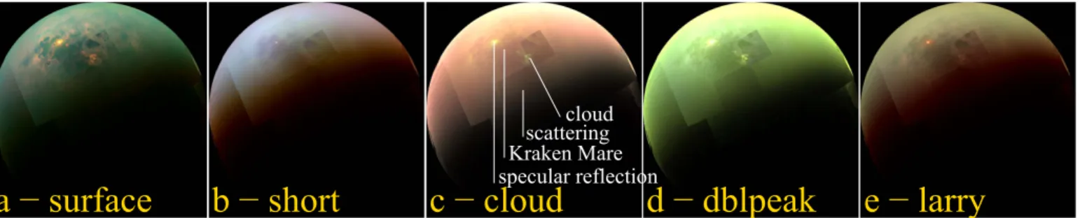
Figure 1.Five different color scheme renditions of a mosaic of Titan data from the VIMS instrument on Cassiniʼs T104 ﬂyby, which occurred on 2014 August 21. In panel(a), we show a color scheme designed to show surface spectral diversity (red=5 μm, green=2 μm, blue=1.3 μm) ﬁrst used by Barnes et al. (2005). Panel

(b) shows a combination of short wavelength surface windows (red=1.58 μm, green=1.08 μm, blue=0.93 μm) after Barnes et al. (2009). The middle panel, (c),

shows a color scheme designed to bring out atmospheric features such that clouds are white, haze is pink, and surface is green(red=2 μm, green=2.7 μm, blue=2.6 μm) from Grifﬁth et al. (2005). Panel (d) renders a view using Titan’s double-peaked 2.7/2.8 micron window (red=2.8 mm , green=2.7 μm,

blue=2.0 μm). Panel (e) at right shows the surface color scheme developed by Soderblom et al. (2007) (red=2 μm, green=1.58 μm, blue=1.28 μm).

9

Of course actual, physical photons do not have varying amplitudes. Our treatment of photons by referring to their“amplitude” is equivalent to what other Monte Carlo models might call a“photon packet” and corresponds to the aggregate behavior of a large number of photons and not to an actual single individual photon.

(4)

single initial photon ID number, each photon is entirely independent of every other photon, not relying on them for any previous knowledge of position or wavelength. Aspect (1) allows for ambitious models with high photon counts and therefore high signal-to-noise ratios (S/Ns), and aspect (2) allows each photon to proceed in parallel disregarding when or on what processor it is running.

The simplest built-in photon generator, photonge-nerator_square, implements a regularly spaced raster of photons with a given side length in kilometers, number of rows and columns n, and list of w different wavelengths. Every photon generator knows its size—the total number of photons that it expects to generate(n2w). The primary loop then starts a long integer iterator i at i=0 and runs through to the photon generator size, passing i, the photon ID number, to the generatephoton() method at the beginning of the loop. This method then determines the wavelength to be the entry in the input list corresponding to the integer value of i/n2. Then, using the remainder r≡i %n2, the row number comes from the integer value of r/n and the column from the remainder r%n. From the row and column number, we determine the initial y and z coordinate locations for the photon. The photons’ initial directions are all the same: –x for photongenerator_ square (though the initial direction could be assigned differently in an updated photon generator, to come from a point source like the Sun for instance instead of being parallel). The output of generatephoton() is an instance of the photonclass that knows its own three-dimensional(3D) vector position, its direction, and its “amplitude” (a measure of what fraction of the virtual photon has been previously absorbed— which of course does not really happen for a single photon, so our photon class might more accurately be thought of as a bundle of photons).

This backwards approach certainly takes a few extra CPU cycles than a forward calculation of y, z, and wavelength in a triple loop. But it reduces memory accesses and storage and allows threads to run independently and for photon ID numbers to run unordered and randomly as assigned by the parallelization.

2.1.3. Detectors

In SRTC++, detectors are implemented as an abstract class—hence, any different kind of detector could be created as

might be helpful to solve any particular future problem. To start, we created a simple detector called colorCCD. A colorCCDknows its position and the direction in which it is pointed. It has a virtual two-dimensional(2D) CCD array with multiple planes to allow for different wavelengths that are calculated simultaneously.

Distinct from existing 1D codes, which typically have as their output a spectrum that results from a particular atmosphere and input geometry, colorCCD records images (like those in Figure 2). Pixels in the image correspond to

different locations on the target planet (or off its limb) and therefore to different local incidence, emission, and azimuthal angles. Because the SRTC++ treatment is 3D, conditions in one area may affect nearby pixels in the colorCCD.

SRTC++takes a vector of detectors as input. It follows that it can use the same radiative transfer calculation to update any number of detectors during a single run. Figure2, for instance, was created in a single SRTC++ conﬁguration that used 36 different detectors arrayed around Titan’s equator every 10°.

For testing purposes (see Section 3), we also introduce a

more complex detector: the elephant detector. It never forgets photon histories. Rather than store the full history of a billion photons, though, elephant detectors have separate colorCCDs for each possible photon scatter path topology. We denote each photon history using a“0” for surface scatters and a “1” for atmospheric scatters. We end up with one colorCCDfor just surface scatters(__0) and one for just one atmospheric scatter (__1). We store each scenario separately for double scatters: surface then atmosphere(_01), atmosphere then surface (_10), and photons that scatter twice off the atmosphere (_11). Although elephant formally tracks surface-then-surface (_00) scatters, too, in practice there should not ever be any of these for spherical planets(though there would be if SRTC++ modeled topography—future work). In general, there should be 2n different colorCCDs per scattering order n(e.g., for n=3: 000, 001, 010, 011, 100, 101, 110, and 111). Elephants allow the user to set the maximum scattering order of which to keep track.

2.2. Main Program Loop

Independent parallel execution threads each start with a photon ID. From this ID, the photon generator determines the

Figure 2.We show here synthetic images from SRTC++ showing output from a Tomasko et al.(2008) Titan atmosphere with a gray surface bitmap alternating

between albedo of 0.03 and 0.20. The colormap is that from Barnes et al.(2007), which uses 5.0μmas red, 2.01μmas green, and 1.3μmas blue. The images show

the expected phase behavior, bright at opposition and inferior conjunction, and dimmer at maximum elongation. The pleasant Titan orange color is fortuitous based on the assumed gray surface, one that does not match that of actual Titan in the near-infrared. The surface albedo pattern for thisﬁgure comes from a small jpeg ﬁle produced in GIMP(like Photoshop) by writing black text on a white background, but SRTC++ can import any raster image of atmozone albedos.

(5)

initial position, direction, and amplitude for the photon in question and sends it into the main program loop.

The main loop is as follows:

(1) plots out the photon’s path forward and backward from its present location, turning that path into a 1D photon traverse through the atmosphere (details in Section 2.2.1);

(2) generates a random excursion for this photon in scattering optical depth spaceτscat(details in Section2.2.2);

(3) translates that random τscat into a physical location for

scattering along the photon traverse (details in Section 2.2.3)—allowed types of scatter are surface,

atmosphere, or space(the latter indicates that the photon has escaped the atmosphere, in which case its amplitude is updated to 0.0);

(4) updates the detectors (details in Section2.1.3) based on

this scatter; and

(5) attenuates the photon’s amplitude by the single-scattering albedo at the scatter location, and updates the photon’s direction based on the local scattering phase function (details in Section 2.2.4).

The resulting new photon position, direction, and amplitude then inform the next iteration of the loop. Each thread continues calculating its photon’s path through scattering events until that photon either ﬂies off into space or its amplitude becomes identically 0.0 (as would happen if the albedo were zero either somewhere in the atmosphere or at the surface), at which time the loop terminates and the thread asks for a new photon ID to calculate.

We describe the details of each of these steps in the following sections.

2.2.1. Photon Traverse

A photon traverse class instantiation translates the photon’s 3D position and direction into a 1D path. The path is centered on the photon’s present location, and we parameterize the distance from that location as d such that negative values are behind the photon and positive values are ahead of it. Armed with this coordinate collapse, we then can determine the atmospheric conditions at any point along the photon’s traverse.

Speciﬁcally, the photon traverse looks up which atmolayer and atmozone corresponds to each value for d. The most important conditions that we need are the volume extinctions κ(λ) at each point. We then numerically integrate that extinction (using qromb from Press et al. 1992) along the photon’s

traverse to calculate the cumulative τ between the photon’s present position and each position d. While the original IDL code on which SRTC++ builds uses an analytic approximation to the Chapman Integral (Smith & Smith 1972), we instead

evaluate the integrated optical depth numerically. While the numerical approach slows program execution, Checlair et al. (2016) shows that the compromises inherent to the (Smith &

Smith 1972) approximation in puffy atmospheres like Titan’s

result in 10% systematic errors. It follows that we ﬁnd the

slow-but-accurate numerical calculation preferable.

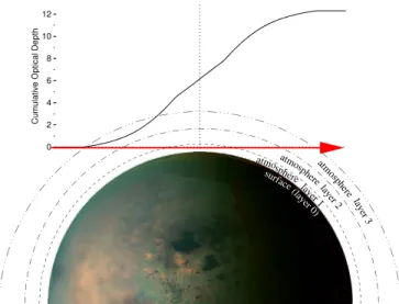
Figure 3 shows an example of how we calculate such an integral. The red line represents the photon traverse next to Titan (a near-grazing impact parameter starting from deep space for this particular photon), and the plot above the red line

shows the integrated haze optical depth at each point along the traverse. We take advantage of this knowledge of the integrated optical depth along the path for Steps 3 and 5.

2.2.2. Generating Random Optical Depths

We need to calculate a location where a photon might scatter in optical depthτscat space. The probability of it scattering at

lowτ is much greater than that at higher τ. (By higher τ, more of the photons have been already scattered out of the beam.) Achieving this aim requires the ability to generate random numbers between 0.0 and +¥ with an exponentially decaying distribution as e− τ.

To do so, we follow Press et al.(2007). First, we generate a

random number frandom between 0.0 and 1.0 using a modiﬁed

version of the Numerical Recipes routine Ranq1 Press et al. (2007). The modiﬁcations allow for parallelization by creating

different instances of the random number generator (seeded with different initial values) for each thread so that they do not interfere with one another. To get the appropriate random τrandomwe then set

f

ln . 1

random random

t = - ( )

2.2.3. Determining the Scattering Location

Having generated a random scatter location along d in τ space(at τrandom), we then need to invert the τ versus d plot in

Figure3 to determine the value of d corresponding toτrandom.

From d, we then infer the precise location in 3D space where the scatter will occur. SRTC++ determines the appropriate

drandom for the random input τrandom numerically using the

Ridders’ Method zero-ﬁnding routine zriddr from Press et al.(1992).

Figure 3.Thisﬁgure shows a stylized representation of an example photon traverse through Titan’s atmosphere. The plot shows the cumulative optical depth as a function of distance along a photon traverse indicated by the red ray. SRTC++uses this type of cumulative optical depth function within a photon traverse to both calculate net atmospheric opacity and to ascertain the location in physical space at which a scattering event occurs, translating from optical depth space. We do that by generating a random photon optical depthτrandomat

which the next scatter occurs from Equation(1) and then tracing that τrandomto

its corresponding location along the traverse in this plot. This particular photon’s photon traverse heads in from deep space, encounters Titan’s outer atmosphere, and then continues down before reaching a closest approach in the troposphere but above the surface. It then heads back out into space. The breaks in slope occur at the interfaces between atmospheric layers as speciﬁed in the Tomasko et al.(2008) atmospheric model.

(6)

2.2.4. Updating the Detectors

After the scattering location has been determined, but before we determine the result of the scatter itself (i.e., the photon’s direction and amplitude moving on from this scatter), we update the detector to reﬂect the response that it would see from this scattering event (Yusef-Zadeh et al. 1984; Dupree & Fraley 2012; Jonsson 2006). This step represents the critical

insight of our Monte Carlo approach: instead of a complete Monte Carlo simulation of light scattering, in which only a very few photons would ﬁnd their way to the detector, we instead accumulate contributions of each photon at the detector as generated by each scattering event. And then we throw away the the Monte Carlo photons after they leave Titan’s atmosphere to avoid double-counting. This approach has come to be known as the “peeling-off” technique.

So, let us restate this critical insight in another way. We use the Monte Carlo photons pinging around through the atmos-phere to determine amplitudes, locations, and geometries for scattering. But we never record the results of the primary photon itself at any detector. Every photon eventually makes its way out of the atmosphere, at which time we ignore it and move on to the next photon to be calculated. Instead at the instance of each scattering, and separately for each detector, we calculate the explicit contribution that the particular scattering in question would have at those detectors. It follows that the detection step is not Monte Carlo but instead is determinitive allowing for efﬁcient use of computation power.

The detector is invoked with a call that passes a photon—the photon with its location as the location of the scatter but with the direction of the photon prior to this particular scattering event. The detector then calculates the relative scattering angle fdbetween its position and the photon, recording the effective

charge c received at the detector based on the photon’s initial amplitude An, the scattering phase function p(fd), the optical

depth between the scatter and the detector τoutbound, and the

single-scattering albedo of the atmosphere at the point of scatter ω (note that we treat scattering and gaseous absorption together such thatω represents both components)

c x y( , , l)+=Anw fp( d)e-toutbound . ( )2 We do this increment separately for each of the detectors in the vector set up for this particular run.

Then, at the end of the entire SRTC++ run when all of the photons areﬁnished, we calibrate the detector into I/F by

I F c x y 1 , , 3 2 ps l = ¡ ( ) ( )

whereσ represents the number of photons incident per square kilometer according to the photon generator andϒ is the colorCCDsampling in kilometers per pixel.

2.2.5. Calculating a New Direction after Scattering

Lastly, for each photon, SRTC++ executes the scattering in a Monte Carlo fashion. We decrease the photon’s amplitude according to the single-scattering albedo of the atmosphere. SRTC++ calculates the new direction by (1) using the phase function to calculate a cumulative distribution function (fraction of scattered light scattered by an angle less than or equal to the ordinate), (2) inverting that cumulative distribution function into angle as a function of fraction, and (3) interpolating the inverse cumulative distribution function to

find the right new angle. Step 3 involves generating a random number in the usual uniform 0.0–1.0 variate fashion, finding where that value would fall in the inverse cumulative distribution function, and then interpolating to find the actual scattering angle implied. Because generating and inverting the cumulative distribution in Steps 1 and 2 depend only on the phase function, we calculate the inverse cumulative distribution functions prior to entering the primary code loop and then all threads share access to the results. Importantly, this approach allows for use of arbitrary phase functions and/or different phase functions in different portions of the atmosphere—we have no requirement that a phase function be decomposable into Henyey–Greenstein or polynomial expansions.

Once we have decided upon a scattering angle, we generate a random azimuth between 0 and 2π. Then comes a kind of tricky part. The scattering angle and azimuth are valid for a coordinate system oriented along the direction of travel of the photon prior to the scattering event. So we transform the initial x, y, z-basis direction vector into one in this new reference frame where the photon travels in+x prior to the scatter. Next, we use the new random scattering angle and azimuth to determine the photon’s outgoing direction after the scatter, but still in the reference frame based on the direction prior to the scatter. Lastly, we transform this outgoing vector back into x, y, z-space and send this post-scatter photon back around the loop for another round.

3. Validation

Any new radiative transfer scheme can only start to be trusted after it faithfully reproduces known endmember test cases. To that end, we use a series of validation test cases to verify that SRTC++ reproduces known cases at a satisfactory level. We use analytic and existing numerical plane-parallel models as our primary comparitors due to their accuracy at high optical depths.(Optically thin and single-scattering approxima-tions to spherical atmospheres (i.e., Rages & Pollack 1983; Squyres et al.1985) might also be relevant in future contexts.)

3.1. Lambertian Surface and Thick Atmosphere The first, simplest check that we run verifies that bare surfaces and infinitely deep atmospheres modeled with SRTC+ +yield comparable answers to analytical results.

For the surface case, we use an albedo equals 1.0 Lambert sphere in combination with an extremely tenuous 1×10−6 optical depth atmosphere. We veriﬁed that this setup produces an average I/F of 2/3 when integrated across the entire disk from 0° phase.

We next compare SRTC++’s results for a high-optical-depth atmosphere 30-km thick(here assumed to be τtotal=5.0 with

uniform extinction for testing purposes—higher τ takes longer to calculate with diminishing returns) to the theoretical results for an plane-parallel, optically thick atmosphere as calculated by Chandrasekhar(1950). Chandrasekhar (1950) shows that

I 0, 1 F H H 4 4 0 0 0 m w m m m m m = + ( ) ( ) ( ) ( )

where I is the incident intensity, F is the resultingﬂux ﬁeld, ω is the single-scattering albedo, andμ and μ0are the cosines of the

angles of the observer and the source(the Sun) with respect to the zenith direction(Chandrasekhar (1950), Equation (26)–(118).

(7)

We rewrite Equation(4) to switch out μ and μ0in favor of

αs instead, which equate to the number of traversed atmo-spheres in the relevant geometry from a plane-parallel atmosphere. So e 1 1 cos 5 a m = = ( ) and I F H H 0, 1 4 0 . 6 a _w a a a a a = +  ( ) ( ) ( ) ( )

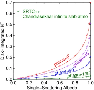
We show the resulting comparison of numerical integrations of Equation(6) over the full disk, as compared to results from

SRTC++, in Figure 4 (see also tabulations of brightness

distribution across the disk in this case from Table 3 in Dlugach & Yanovitskij 1974). We assume an isotropically scattering

atmospheric phase function in both cases for simplicity(we use more complex atmospheric phase functions in later tests outlined below). Figure 4 shows four different curves in different colors—one for the spherical planet as viewed at four different phase angles (0°, 45°, 90°, and 135°). The SRTC++ result closely tracks the theoretical result of the Chandrasekhar slab all the way up to just below a single-scattering albedo of 1.0 where the theoretical value no longer applies. It follows that SRTC++ works for this simple phase function in a multiple-scattering regime.

3.2. Atmosphere and Surface

For the next veriﬁcation step, we compare SRTC++ results to those of a more general semianalytic model. We use a model derived by one of us (BKJ) from Thomas & Stamnes (2002)

and initially used in Vixie et al.(2015). The model separately

calculates I/F contributions from different scattering histories involving at most one atmospheric scatter. Speciﬁcally, we

look at the terms that correspond to: (1) photons that make it through the atmosphere, scatter off the surface, and make it all the way out unscathed; (2) photons that scatter off the atmosphere once and then back to the detector; (3) photons that scatter ﬁrst off the atmosphere, and then off the surface, before being detected; and (4) photons that scatter off the surfaceﬁrst, then scatter off the atmosphere on their way out. Using elephant detectors in SRTC++, then, we can compare the Monte Carlo result directly to the semianalytical result for each scattering history individually.

In this comparison, we assume a uniform-extinction, 30-km-thick atmosphere with haze that scatters according to the Tomasko et al. (2008) phase function below 80 km. For

purposes of the test, we assume optical depthsτ and single-scattering albedos ω as shown in Table 1. These values are consistent with both Huygens results(Tomasko et al.2005) and

Cassini measurements of atmospheric transmission within Titan’s spectral windows (Barnes et al. 2013; Hayne et al.

2014; Maltagliati et al.2015a). As we intend to test our model

and not simulate actual Titan in this particular instance, we set the surface albedo A=1.0 and we ignore gaseous absorption. On the SRTC++ side, this model run uses 22,606,068 photons, illuminating the full disk of Titan. We install 18 different detectors, each elephants in this case, spread out in phase angle from the Sun from 0° to 170° in 10° increments. This run took overnight to complete.

3.3. One Scatter at Surface(__0)

Theﬁrst term corresponds to scatter only from the surface,

I

F A s i e, , e 7

i e

__ 0 ₌_p _F _f _-_{t a} ₊_a

( ) ( ( ) ( )) ( )

where i is the incidence angle, e is the emission angle, andf is the phase angle. I__ 0corresponds to the intensity at the detector

for light that only reﬂects off the surface one time and that is not extincted by the atmosphere on the way in or the way out. We convert this to the more easily interpreted I/F by dividing by the solarﬂux F. A is the surface albedo.F (s i e, , f) refers to the surface phase function (hence the s), which could potentially be a function of the incidence, emission, and phase angles. Finally, τ is the one-way atmospheric optical depth at normal geometry(i.e., looking straight down or up through the atmosphere), and the α functions of incidence (i) and emission (e) correspond to the number of atmospheres traversed by photons in this geometry under the plane-parallel approx-imation—so i

i 1 cos

a( )= .

Figure 4.We show here a comparison between disk-integrated I/F values for an optically thick atmosphere viewed at 0°, 45°, 90°, and 135° phase. We assume an isotropic atmospheric scattering phase function. The results calculated by SRTC++(asterisks) and by numerical integration of Chandrase-khar’s slab equation (solid lines, from Equation (6)) substantially agree with

one another for this simple case.

Table 1

Atmospheric Parameters Assumed for the Orange-rind Atmosphere Validation Described in Section3.2

Wavelength Optical Depth Single-scattering Albedo 0.93μm τ0.93=3.2 ω0.93=1.00 1.08μm τ1.08=2.5 ω1.08=0.99 1.28μm τ1.28=2.1 ω1.28=0.98 1.58μm τ1.58=1.45 ω1.58=0.96 2.0μm τ2.0=1.02 ω2.0=0.77 2.68μm τ2.68=0.8 ω2.68=0.507 2.78μm τ2.78=0.8 ω2.78=0.463 5.0μm τ5.0=0.3 ω5.0=0.4998

(8)

We show the results for the 1-scatter from surface case in Figure 5. In this plot and the other comparisons to the semianalytical model, we generate our error bars empirically. For each geometry (i.e., i=e=20°), we collect all of the pixels in the colorCCD that match the incidence and emission to within a given tolerance (here we use 5°). We assign the asterisk SRTC++ value in Figure5to the average of the pixels in that collection, and the error to their standard deviation. Because that collection includes a wide diversity of phase angles between f=0° and f=i+e, this approach over-estimates the errors. But because we compare the same set of pixels in both the SRTC++ and semianalytical cases, the validation comparison remains valid. SRTC++ and the semianalytical approach agree within very tight tolerances— not entirely unexpected as this case is particularly simple compared to multiple-scattering cases.

3.4. One Scatter in the Atmosphere(__1)

In the semianalytical model, light that scatters only once in the atmosphere has an intensity of

I F p i e e i e e , , 1 i e 8 __ 1 _pw _f a a a = + -t a a - + ( ) ( ) ( ) ( )( ) ( ) ( ( ) ( ))

where new parameterω corresponds to the atmospheric single-scattering albedo and new function p to the atmospheric scattering phase function, which potentially depends on the incidence, emission, and phase. We compare the results of this equation and that of SRTC++ in Figure 6.

The resulting plots show more complicated behavior than those for the surface-only case. At longer wavelengths(i.e., at 5μm), the expected I/F increases monotonically with viewing angle(we assume that the incidence angle equals the emission angle so as not to end up with 92different lines in the plot) as the higher path length increases the slant optical depth. For shorter wavelengths, though, like at 0.93μm, the situation gets

more complicated. The i=e=0° case shows up as the dimmest. But instead of a monotonic increase, the 0.93μmI/F peaks at i=e=20° before decreasing and later increasing again toward very high incidence and emission. The more highly forward-scattering phase function at shorter wavelengths causes the disparity. Note the interesting case where the two blue curves, i=e=20° and i=e=70° both have the same I/F at 0.93μmbut then diverge as they head toward longer wavelengths and lower optical depths. This effect is a bit unintuitive, but shows up in both models as SRTC++ and the semianalytic model track each other well up to i=e=70°.

At i=e=80°, though, the two models disagree. Presum-ably, this discrepancy results from applying the semianalytic model, which assumes plane-parallel geometry, beyond the point where it produces physical results.

3.5. Two Scatters: Atmosphere, then Surface(_10) We also explore the behavior of the orange-rind plane-parallel atmosphere in SRTC++ where photons experience two scatters. While SRTC++ tracks the signal independently for any number of scatters, and where they occur, with elephant detectors, here we look at just the two-scatter case for ease of comparison to the semianalytical model. This case is quite a bit trickier for the analytical model in that we need to integrate over the upward hemisphere as seen from the surface, which encompasses all of the possible paths that the photon could take between its initial atmospheric scatter and its eventual surface scatter. We parameterize that hemisphere in terms of the zenith distanceζ and the azimuthal angle θ in the sky as seen from the surface scatter point. The hemispherical integral becomes one overζ and θ such that

9 I F e p i i i e d d _ , , , , . e s 10 0 2 0 2

ò

pw z q a a a z z q q z = ´ - F ta p p -( ) ( ) ( ) ( ) ( ) ( ) ( )

where now both the phase function for the surfaceΦsand that

for the atmosphere p drive the ﬁnal ﬂux. We compute this

Figure 5. This ﬁgure is the ﬁrst of four plots comparing SRTC++ to a semianalytical model(described in Section3.2) at different scattering orders.

For each of these four plots, we assume a 30-km deep orange-rind atmosphere with the scattering phase function of Tomasko et al.(2008) for below 80km (to

test SRTC++’s use of complex phase functions). The optical depth τ and single-scattering albedoω were chosen to be representative of Titan within each window. This particular plot shows I/F as a function of wavelength within Titan’s near-infrared atmospheric windows for light that only scatters off the surface and not from the atmosphere. Both approaches arrive at the same answers for this(relatively simple) case.

Figure 6.We again compare SRTC++ results to semianalytical results, in this case for photons that only scatter one time within the atmosphere. The solid line plots the result of Equation(8) while the asterisks with error bars show

SRTC++’s answer. The analytical model assumes plane-parallel geometry, and hence is well outside its range of validity by the time i=e=80°.

(9)

nested integral numerically. If you try it yourself, take care to ensure that your inputs to the phase functions appropriately correspond to the angles between the incident and intermediate vector for the atmospheric phase function, and for the intermediate to emission vector for the surface phase function. The result of that numerical integration of Equation (9) we

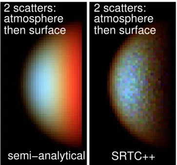
show in Figure7, along with the equivalent SRTC++ answer. The models track together across 80° in incidence and emission. In fact, they track surprisingly well—at least partially as a result of the squat 30-km atmospheric extent imposed on the SRTC++ calculations for the precise purpose of testing their comparison to the plane-parallel semianalytical model.

We show a spatial example of the results in Figure 8 as viewed from the detector with 90° phase. The bright red near the terminator of the semianalytical model is bogus as the very high incidence angle near the terminator invalidates plane-parallel results. The pixel-to-pixel noise in the SRTC++ image is real—the more photons in the simulation, though, the higher the signal-to-noise gets.

3.6. Two Scatters: Surface, then Atmosphere(_01) The complement of Equation (9), photons bouncing ﬁrst

from the surface then from the atmosphere and to the detector, is given by I F e p i e e e d d _ , , , , . 10 i s 01 0 2 0 2

ò

pw z q a a a z z q q z = ´ - F ta p p -( ) ( ) ( ) ( ) ( ) ( ) ( )

The hemisphere of integration remains the sky from the surface point, but now the intermediate segment comes after that surface scatter instead of before it. Owing to the similarity between Equation(9) and Equation (10), the two equations yield the same

answer regardless of the atmospheric phase function in the case

where the surface phase function is Lambertian. The I/F differs between the _10 and _01 cases under non-Lambertian surface phase functions (we see a difference when using an isotropic surface phase function, for example).

Given the assumed Lambertian surface scattering we see results in Figure 9 for the surface-then-atmosphere case are consistent with those from the atmosphere-then-surface case. The noise in the SRTC++ calculations is higher here, though, because of the highly forward-scattering nature of Titan’s haze particles (from the Tomasko et al. (2008) phase function).

Those fewer photons whose direction after their surface scatter brings them to within a few degrees of being pointed at the detector contribute more strongly to the detected intensity; hence the statistics of those relatively smaller numbers yields higher noise in Figure7than in Figure9. Overall, the results of the SRTC++/semianalytical comparisons give us conﬁdence in the SRTC++ calculations.

3.7. Plane-Parallel Titan

For aﬁnal validation, we compare SRTC++ calculations to those of the existing Spherical Harmonic Discrete Ordinate Method plane-parallel radiative transfer model from Evans (2007) adapted for Titan by Hirtzig et al. (2013). We ran the

Hirtzig et al.(2013) model without gaseous absorption and for

endcases with surface albedo A=0.0 (all atmosphere) and A=1.0. For purposes of validation of SRTC++, the Hirtzig et al. (2013) model run assumes a Tomasko et al. (2008) Figure 7. We plot here the results of double-scattering radiative transfer

calculations for the I/F as a function of wavelength for a Titan-like orange-rind atmosphere. In particular, here we only track those photons thatﬁrst scatter off of the atmosphere, and then scatter off the surface to the detector. Because only a fraction of the total photons simulated experience this precise history, the S/ N in the SRTC++ data has decreased relative that in Figure5. However the results agree well between the Monte Carlo SRTC++ and the semianalytical model from Equation(9).

Figure 8.These images show the spatial results from the _10 calculations described in Section 3 for both the semianalytical model (left, from Equation(9)) and SRTC++ (right). The relatively low S/N evident in the

pixel-to-pixel variation results from(1) selecting only that fraction of photons that experience the specific history _10 (i.e., ones that first bounce off of the atmosphere, then bounce off of the surface and arrive at the detector) and (2) using this many photons allowed us to sufficiently demonstrate that SRTC++ satisfactorily reproduces known plane-parallel results as shown in Figure7. Running additional photons always improves the S/N, but takes progressively longer owing to the S/N’s dependence on the square-root of the number of photons input. The colors map red to 5.0μm, green to 2.0μm, and blue to 1.3μm. This image depicts a uniform sphere of albedo 1.0 illuminated from the left at 90° phase angle. Hence the strong red signal in the semianalytical case comes from geometry near the terminator with high incidence angle i—a regime in which its plane-parallel assumptions break down.

(10)

atmospheric proﬁle and haze phase functions, with interpolated single-scattering albedos between the high and low layer values within the middle atmospheric layer.

We then set up SRTC++ with an analogous atmosphere, but compressed vertically by a factor of 100 to more closely emulate the plane-parallel assumptions of the Hirtzig et al. (2013) model. We use two separate runs of 135,636,528

photons each, one for A=0 and one for A=1, with the photon generatoremitting photons concentrated on areas with the appropriate geometry. We ran each run on a separate computer over a 3-day weekend.

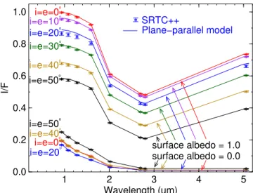
Figure10shows the resulting intercomparisons. The Hirtzig et al.(2013) plane-parallel model and SRTC++ both agree from

i=e=0° through i=e=50°. 4. Duration

A drawback to Monte Carlo methods for 3D radiative transfer is that they tend to be slow. We have offset this weakness with parallelization and a fast implementation in C+ +, but undoubtedly we can optimize further. In the meantime, we show an indication of how fast SRTC++ runs right now in Figures 11and12.

Figure 11 plots the computational speed in terms of throughput in photons per second as a function of the number of CPU cores that we use in the calculation. These runs executed on a dual 8-core (16 total cores) 3.2 GHz machine using the Titan model atmosphere from Section3.7with 57800 photons per run. As we designed the SRTC++ algorithm for each photon to calculate almost entirely independently from the others, the program is“embarrassingly parallel” in that we see only minor degradation in throughput per core even up to 16 cores executing simultaneously.

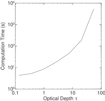
Atmospheric optical depth τ also signiﬁcantly affects compute time. In Figure 12, we show the computation time for 57800 photons in uniform-extinction orange-rind atmo-spheres of differing optical depths. Computation times increase greater-than-linearly with optical depth, so while radiative transfer on Titan at 2μm where τ=1 proceeds rapidly,

calculations at visible wavelengths where τ∼10 take considerably longer.

5. Application

We developed SRTC++ to complement existing plane-parallel codes. Those models do a good job of modeling Titan near-IR reﬂectance spectra in geometries i60° e60° where the plane-parallel approximation holds. SRTC++ will model spatial problems, creating simulated images to char-acterize near-limb and near-terminator geometries, imaging resolution and surface nonuniformity, surface phase functions, specular reﬂections, and other problems.

Figure 9.Thisﬁgure represents our last comparison between SRTC++ and the semianalytical model. In this two-scatter, surface-then-atmosphere case, the lines show Equation(10) and the asterisks with error bars show the SRTC++

result. Although the semianalytical values match those from the atmosphere-then-surface case(Figure7), the higher SRTC++ noise here (i.e., lower S/N)

results from Titan’s highly forward-scattering haze particles’ phase function (see the text).

Figure 10.This plot compares SRTC++ results to those from the Hirtzig et al. (2013) plane-parallel model for a Tomasko et al. (2008) Titan atmosphere with

no gaseous absorption. The top set of points correspond to a model with surface albedo A=1.0, while the lower plots show results for a black A=0 surface.

Figure 11.In thisﬁrst of two benchmark graphs, we show SRTC++ calculation speed as a function of the number of CPU cores used in the calculation. The throughput is nearly linear, with a small concave-down aspect resulting from the computation overhead of running in parallel. On the whole, the system scales well in this CPU regime. The gray dashed line provides a reference to guide the eye in assessing deviations from straight-line behavior.

(11)

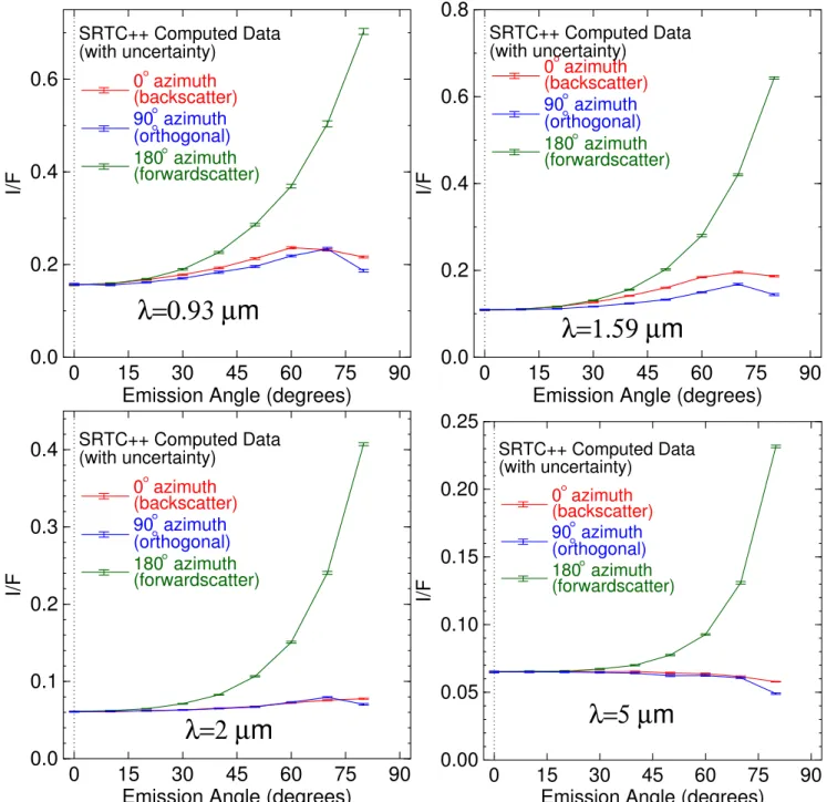
To illustrate SRTC++’s capabilities, we use it to calculate emission phase functions for Titan, which we show in Figure13. Complementary to our earlier ﬁgures, like Figure 7, which assumes specular geometry with an incidence angle equal to the emission angle, Figure 13uses a ﬁxed incidence angle of 60° and varies only the emission angle. If you were a spacecraft starting right above the illuminated point on the 4PM afternoon equator, you could acquire an emission phase function by staring at that point as you moved around the moon. But you could do so in any direction. To show how that direction would affect your measurements, we show the emission phase function as if you were in a prograde equatorial orbit heading toward the terminator and looking back (dark green), as if you were in a retrograde equatorial orbit heading toward noon(red), and as if you were in a polar orbit(blue). The differences between these azimuths result from the backscattering (red) and forward-scattering(dark green) properties of Titan’s atmospheric haze.

The SRTC++ algorithm as we describe it here represents an initial ﬁrst-cut that can start to address useful problems. However, we plan many improvements and optimizations in the future as needed. For instance, right now SRTC++ only accounts for gaseous absorption within the atmospheric single-scattering albedo parameter. As a future improvement, we intend to separately treat haze and gas opacities, using correlated-k coefﬁcients to simulate VIMS’ rather coarse spectral resolution elements. SRTC++ will probably never be the best choice for large problems that require high spectral resolution, however, like computing radiative atmospheric heating rates.

While at present SRTC++ includes a canned Tomasko et al. (2008) atmospheric model, Doose et al. (2016) since described

improvements on the Tomasko et al. (2008) atmospheric

model. It follows that while we will maintain the present model capabilities, future applications of SRTC++ will preferentially assume the Doose et al.(2016) Titan haze scattering properties.

The surface phase functions included in SRTC++ now(just isotropic and Lambertian) are azimuthally symmetric. How-ever, Buratti et al.(2006) showed a long time ago that Titan’s

surface does not obey a Lambertian law but rather shows signiﬁcant backscattering properties. Buratti et al. (2006) used

a Henyey–Greenstein surface phase function. But with better knowledge of diffuse atmospheric illumination from SRTC++, along with an additional 12 years of VIMS data, we hope to infer more detailed surface properties on Titan’s various terrains from their phase functions using SRTC++.

Specular reﬂections from Titan’s lakes and seas (Stephan et al. 2010; Barnes et al. 2011; Soderblom et al. 2012) will

prove a separate challenge. Purely specular surfaces will require separate calculations of two different paths to each detector through the specular point. Specular reﬂections from a roughened surface (like the wavy Punga mare described in Barnes et al.2014), however, can be modeled with the present

construction via particular non-azimuthally symmetric phase functions.

Because of its inherently 3D structure, SRTC++ can also simulate atmosphere-only phenomena. In particular, limb observations of atmospheric haze, stellar and/or solar occulta-tions, and Titan’s winter south polar cloud (West et al.2016)

would be amenable to analysis using SRTC++.

Thinking bigger-picture, SRTC++ can also be applied to the photometric and spectroscopic properties of exoplanets. Direct detections of planets (e.g., Kalas et al. 2008) measure

disk-integrated planetary properties; SRTC++ could be used to accurately forward-compute expected photometric behavior of such planets as a function of phase as they orbit their parent star (Cahoy et al.2010). SRTC++ might also be proﬁtably applied

to transit spectroscopy of planets (Hubbard et al. 2001)—

particularly those with thick and/or extended Titan-like atmospheres (Checlair et al. 2016). The high slant optical

depths in such cases(Fortney2005), potentially combined with

east-west and equator-pole inhomogeneities (Fortney et al.

2010), lend themselves naturally to SRTC++’s explicit and

accurate approach.

While not yet incorporated, the detector design allows for future intelligent coaddition of colorCCDʼs to maximize CPU time. For instance, after a single run, if the user desires a higher S/N, then results from a second run could be coadded with those of the ﬁrst run. Similarly, separate instances of SRTC++ could be run on different computers, only to have their colorCCD results combined later to amalgamate separate computers as a greater cluster.

Right now, SRTC++ uses OpenMP for parallelization. OpenMP unlocks all of the cores on a single computer for use. A future improvement might be to use the alternate parallelization scheme MPI, which allows networks of computers to all contribute their CPU cores toward a particular problem. Such a change would enable SRTC++ to run on large supercomputers that do not use shared memory as well.

The compilation process might be facilitated by use of a photon generator more sophisticated than that of our photo-ngenerator_square. The raster pattern performs much better than an entirely random photongenerator in that its noise drops as N−1as opposed to N-12 (Press et al.2007, page

404). However, it requires that the user decide in advance how many photons to use. It would be straightforward to instead implement a new photongenerator to make use of the Sobol’ (1967) distribution. The Sobol’ sequence is subrandom Figure 12.We plot here the total computation time for an uniform orange-rind

atmosphere with different optical depths. Higher optical depths require much longer to complete; it follows that SRTC++ will be slow when simulating, for instance, radiative transfer through Titan’s atmosphere at optical wavelengths.

(12)

an deterministic, but progressivelyﬁlls in holes left in 2D space such that it could be cut off at an arbitrary point without introducing spatial irregularities (see Press et al. 2007, Figure 7.8.1).

Further speedup may be possible using an exact precompu-tation of the single-scattering component. Because most of the signal in a SRTC++ output comes from singly scattered photons(either __0 or __1), most of the noise comes from that component, too. If the single-scattered components of an elephant detector were assigned as semianalytical values, then the net noise would depend only on the higher-order scattering components. The ultimate result of such a

modiﬁcation would be higher precision results with fewer input photons.

As written, SRTC++ depends on other packages and thus requires specific effort to install on operating system architectures other than that on which we wrote it(FreeBSD). It follows that we provide access to SRTC++ via a whole-disk image of a working FreeBSD system that can be run from a thumb drive or as a virtual machine. You can find that disk image at the SRTC++ github repository located athttps:// github.com/SRTCpp/Code where we also include a copy of the primary source code files (which are also accessible via DOI as doi:10.5281/zenodo.1193815).

Figure 13.These graphs show an example of SRTC++’s capabilities in the form of emission phase functions for Titan at four representative near-infrared window wavelengths. Each uses a single illuminated patch on the surface at the equator with 60° incidence angle. SRTC++ shows the interesting differences in the I/F as a function of emission when viewed at different angles: red shows the emission phase function as viewed from lower phase angles(i.e., toward the Sun), dark green shows the emission phase function at higher phase angles(the forward-scattering regime), and blue shows the emission phase function as acquired from detectors heading north from the illuminated patch(orthogonal to the Sun–Titan–Spacecraft plane).

(13)

The authors acknowledge the support of the NASA/ESA Cassini mission. J.W.B. acknowledges support from the NSF Astronomy & Astrophysics(A&A) Program grant #1313427. S.M.M., E.F.Y., and J.M.S. acknowledge support from NSF grant #1518226. Additional support was provided by Hubble program number HST-GO-12900.003-A from NASA through a grant from the Space Telescope Science Institute, which is operated by the Associate of Universities for Research in Astronomy, Incorporated, under NASA contract NAS5-26555. S.R. is partly supported by the Institut Universitaire de France. S.R. and T.C. also acknowledge ﬁnancial support from the UnivEarthS LabEx program of Sorbonne Paris Cite (ANR-10-LABX-0023 and ANR-11-IDEX-0005-02) and the French National Research Agency(ANR-APOSTIC-11-BS56-002 and ANR-12-BS05-001-3/EXO-DUNES). The authors acknowl-edge Johnathon Ahlers for insights into compiling SRTC++ under Linux. Thanks to reviewer Chris McKay and to editor Thomas Robitaille for constructive comments.

ORCID iDs

Jason W. Barnes https://orcid.org/0000-0002-7755-3530

Brian K. Jackson https://orcid.org/0000-0002-9495-9700

References

Ádámkovics, M., Mitchell, J. L., Hayes, A., et al. 2016,Icar,270, 376

Baes, M., Davies, J. I., Dejonghe, H., et al. 2003,MNRAS,343, 1081

Barnes, J. W., Brown, R. H., Soderblom, L., et al. 2007,Icar,186, 242

Barnes, J. W., Brown, R. H., Turtle, E. P., et al. 2005,Sci,310, 92

Barnes, J. W., Clark, R. N., Sotin, C., et al. 2013,ApJ,777, 161

Barnes, J. W., Soderblom, J. M., Brown, R. H., et al. 2009,P&SS,57, 1950

Barnes, J. W., Soderblom, J. M., Brown, R. H., et al. 2011,Icar,211, 722

Barnes, J. W., Sotin, C., Soderblom, J. M., et al. 2014,PlSci,3, 3

Buratti, B. J., Sotin, C., Brown, R. H., et al. 2006,P&SS,54, 1498

Cahoy, K. L., Marley, M. S., & Fortney, J. J. 2010,ApJ,724, 189

Chandrasekhar, S. 1950, Radiative Transfer(Oxford: Clarendon Press) Checlair, J., McKay, C. P., & Imanaka, H. 2016,P&SS,129, 1

Coustenis, A., Lellouch, E., Maillard, J. P., & McKay, C. P. 1995,Icar,118, 87

Dlugach, J. M., & Yanovitskij, E. G. 1974,Icar,22, 66

Doose, L. R., Karkoschka, E., Tomasko, M. G., & Anderson, C. M. 2016,Icar,

270, 355

Dupree, S. A., & Fraley, S. K. 2012, A Monte Carlo Primer: A Practical Approach to Radiation Transport(Berlin: Springer)

Evans, K. F. 2007,JAtS,64, 3854

Fortney, J. J. 2005,MNRAS,364, 649

Fortney, J. J., Shabram, M., Showman, A. P., et al. 2010,ApJ,709, 1396

Grifﬁth, C. A. 1993,Natur,364, 511

Grifﬁth, C. A., Doose, L., Tomasko, M. G., Penteado, P. F., & See, C. 2012a,

Icar,218, 975

Grifﬁth, C. A., Lora, J. M., Turner, J., et al. 2012b,Natur,486, 237

Grifﬁth, C. A., Penteado, P., Baines, K., et al. 2005,Sci,310, 474

Hayne, P. O., McCord, T. B., & Sotin, C. 2014,Icar,243, 158

Hirtzig, M., Bézard, B., Lellouch, E., et al. 2013,Icar,226, 470

Hubbard, W. B., Fortney, J. J., Lunine, J. I., et al. 2001,ApJ,560, 413

Jonsson, P. 2006,MNRAS,372, 2

Kalas, P., Graham, J. R., Chiang, E., et al. 2008,Sci,322, 1345

Maltagliati, L., Bézard, B., Vinatier, S., et al. 2015a,Icar,248, 1

Maltagliati, L., Rodriguez, S., Sotin, C., et al. 2015b, in European Planetary Science Congress 10,EPSC2015-687

McKay, C. P., Pollack, J. B., & Courtin, R. 1989,Icar,80, 23

Porco, C. C., Baker, E., Barbara, J., et al. 2005,Natur,434, 159

Press, W. H., Teukolsky, S. A., Vetterling, W. T., & Flannery, B. P. 1992, Numerical Recipes in C. The Art of Scientiﬁc Computing (Cambridge: Cambridge Univ. Press)

Press, W. H., Teukolsky, S. A., Vetterling, W. T., & Flannery, B. P. 2007, Numerical Recipes: The Art of Scientiﬁc Computing (Cambridge: Cambridge Univ. Press)

Rages, K., & Pollack, J. B. 1983,Icar,55, 50

Rannou, P., McKay, C. P., & Lorenz, R. D. 2003,P&SS,51, 963

Richardson, J., Lorenz, R. D., & McEwen, A. 2004,Icar,170, 113

Robitaille, T. P. 2011,A&A,536, A79

Rodriguez, S., Le Mouélic, S., Sotin, C., et al. 2006,P&SS,54, 1510

Smith, B. A., Soderblom, L., Beebe, R. F., et al. 1981,Sci,212, 163

Smith, F. L., & Smith, C. 1972,JGR,77, 3592

Smith, P. H., Lemmon, M. T., Lorenz, R. D., et al. 1996,Icar,119, 336

Sobol’, I. M. 1967, ZVMMF, 7, 784

Soderblom, J. M., Barnes, J. W., Soderblom, L. A., et al. 2012,Icar,220, 744

Soderblom, L. A., Kirk, R. L., Lunine, J. I., et al. 2007,P&SS,55, 2025

Solomonidou, A., Coustenis, A., Hirtzig, M., et al. 2016,Icar,270, 85