HAL Id: hal-02912110
https://hal.archives-ouvertes.fr/hal-02912110
Submitted on 5 Aug 2020
HAL is a multi-disciplinary open access
archive for the deposit and dissemination of
sci-entific research documents, whether they are
pub-lished or not. The documents may come from
teaching and research institutions in France or
abroad, or from public or private research centers.
L’archive ouverte pluridisciplinaire HAL, est
destinée au dépôt et à la diffusion de documents
scientifiques de niveau recherche, publiés ou non,
émanant des établissements d’enseignement et de
recherche français ou étrangers, des laboratoires
publics ou privés.
3D rock fabric analysis using micro-tomography: An
introduction to the open-source TomoFab MATLAB
code
Benoit Petri, Bjarne Almqvist, Mattia Pistone
To cite this version:
Benoit Petri, Bjarne Almqvist, Mattia Pistone. 3D rock fabric analysis using micro-tomography: An
introduction to the open-source TomoFab MATLAB code. Computers & Geosciences, 2020, 138,
pp.104444. �10.1016/j.cageo.2020.104444�. �hal-02912110�
Computers & Geosciences 138 (2020) 104444
Available online 15 February 2020
0098-3004/© 2020 The Authors. Published by Elsevier Ltd. This is an open access article under the CC BY-NC-ND license
(http://creativecommons.org/licenses/by-nc-nd/4.0/).
3D rock fabric analysis using micro-tomography: An introduction to the
open-source TomoFab MATLAB code
Benoît Petri
a,b,1,*, Bjarne S.G. Almqvist
c,2, Mattia Pistone
a,d,3aInstitute of Earth Sciences, University of Lausanne, G�eopolis, 1015, Lausanne, Switzerland bUniversit�e de Strasbourg, CNRS, IPGS UMR 7516, F-67000, Strasbourg, France cDepartment of Earth Sciences, Uppsala University, Villav€agen 16, 752 36, Uppsala, Sweden
dDepartment of Geology, Franklin College of Arts and Sciences, University of Georgia, 210 Field Street, Athens, GA, 30602-2501, USA
A R T I C L E I N F O
Keywords:
Microfabric analysis Tensor analysis Micro-tomography X-ray computed tomography MATLAB GUI
A B S T R A C T
The study of rock fabric properties (orientation, planar, linear, anisotropy) is key to unravelling the geological processes that generated them. With advancements in data acquisition and treatment, X-ray micro-computed tomography (μXCT) represents a powerful method to analyse the shape preferred orientation (SPO) of rock- forming elements, including minerals, aggregates, and pores, in the three-dimensional space. After reconstruc-tion and segmentareconstruc-tion of μXCT images, we developed a novel protocol to construct and analyse the fabric tensor, a second-rank symmetric tensor constructed using the orientation and the length of the three characteristic axes of each grain (simplified to a best fit ellipsoid). The analysis of the fabric tensor permits calculation of mean principal directions and associated confidence ellipses, and quantifies the degree of anisotropy (P0) and the shape
(T) of the fabric ellipsoid by eigenvalue and eigenvector analysis.
We implement this method in the TomoFab open-source MATLAB package. The code integrates a graphical user interface (GUI) that allows the visualisation of the full set of ellipsoid orientation, shape, and size. Density plots and contouring can be utilised to identify fabrics graphically, and a full set of fabric parameters can be calculated based on the analysis of the fabric tensor and/or the analysis of each principal direction orientation tensor.
We demonstrate the versatility of TomoFab with synthetic datasets and a field- and laboratory-based inves-tigation of a sample presenting a magmatic foliation and lineation, collected in the Mafic Complex within the lower crustal section of the Ivrea-Verbano Zone (North Italy). In the light of these developments, we stress that μXCT represents a pertinent tool for rock fabric analysis to characterise the SPO of rock components. This approach can be performed parallel or complementary to other rock fabric quantification methods (e.g., AMS, EBSD) and applied to various rock types. TomoFab is freely available for download at https://github. com/benpetri/tomofab.
1. Introduction
A rock fabric (or petrofabric) corresponds to a spatial and geomet-rical arrangement of elements inherent to a rock (minerals, grain ag-gregates, pores, inclusions). This is controlled by compositional layering, grain size variations of minerals, shape preferred orientation (SPO) and crystallographic preferred orientation (CPO) of grains. The study of rock fabrics provides multi-scale insights into various geological
processes such as magma flow (Benn and Allard, 1989; Nicolas, 1992), rock strain patterns (Chopin et al., 2012), and paleo-sediment transport directions (Benn, 1994). The fabric development can be described semi-quantitatively in the field (foliation, lineation), but proper quan-tification requires more rigorous methods (Higgins, 2006). To date, quantitative fabric studies involve electron backscatter diffraction (EBSD; Prior et al., 1999) measurements for CPO determination (e.g., Bascou et al., 2001) and magnetic fabric measurements, such as * Corresponding author. Universit�e de Strasbourg, CNRS, IPGS UMR7516, F-67000, Strasbourg, France.
E-mail address: [email protected] (B. Petri).
1 Development of ideas and software, data treatment, participation to discussions and manuscript writing. 2 Development of ideas, participation to discussions and manuscript writing.
3 Data acquisition and treatment, participation to discussions and manuscript writing.
Contents lists available at ScienceDirect
Computers and Geosciences
journal homepage: www.elsevier.com/locate/cageo
https://doi.org/10.1016/j.cageo.2020.104444
anisotropy of both magnetic susceptibility (AMS) and anhysteretic remanent magnetization (AARM) (Borradaile and Jackson, 2010; Hirt and Almqvist, 2012); AMS and AARM depend on both CPO and SPO (for ferromagnetic minerals) of the magnetic minerals of rocks (Petri et al., 2018). Obtaining the three dimensional SPO is however time-consuming because it requires either serial sectioning or grinding of samples and image analysis (e.g., Bryon et al., 1995). Alternatively, the SPO can be estimated by analysing three or more section planes (slabs or thin sec-tions) at high-angle to one another or by more advanced statistical methods if the observation planes are not mutually perpendicular (e.g., Heilbronner, 1992; Launeau and Robin, 2005; Moreno Ch�avez et al., 2018; Robin, 2002; Shan, 2008). The characterisation of a petrofabric by SPO requires determining the shape and orientation of each individual rock component. Consequently, a fabric can be either weakly developed (i.e., isotropic) with rounded and/or randomly oriented components or strongly developed (i.e., anisotropic) with highly elongated or flattened and strongly aligned components.
The development of micro-computed tomography techniques, using either X-ray or neutron tomography (e.g., Ketcham and Carlson, 2001; Vontobel et al., 2006), provides access to the three-dimensional explo-ration of a rock volume and represents a powerful tool when single grains and/or grain aggregates can be visualised and segmented. Micro-computed tomography has found several applications ranging from fluid flow characterisation in porous media (Islam et al., 2018; Starnoni et al., 2017) to imaging biological matter (Titschack et al., 2018). The size, shape and orientation of each individual object can be extracted (e.g., Som et al., 2013) using Blob3D for instance (Ketcham, 2005b), but this approach requires subsequent statistical treatment. There is a wealth of literature on the statistics of 3D orientation data (Fisher, 1953; Watson and Irving, 1957), which is summarised in several text books (Borradaile, 2003; Fisher et al., 1993; Mardia and Jupp, 2009). Specifically, spherical statistics are mainly obtained by means of vector (or axis) analysis or by analysing the orientation or the fabric second-rank tensors from which several parameters can be used to calculate the properties of the fabrics. While the construction of the orientation tensor is unequivocal (Scheidegger, 1965; Watson, 1966), various approaches to construct a “fabric tensor” have been reported, notably for bone structure characterisation (Odgaard, 1997) and applied to rock fabric quantification (Ketcham, 2005a; Launeau and Cruden, 1998; Launeau and Robin, 1996; Macente et al., 2017; Sch€opa et al., 2015). The different approaches to construct a fabric tensor are: (1) the star length distribution (SLD; Odgaard et al., 1997; Smit and Odgaard, 1998), which probes the grain shape by analysing the length of axes sourcing from a point located in the volume; (2) the star volume dis-tribution (SVD), which reports the volume of a cone that originates from a point located in the volume; and (3) the mean intercept length (MIL; Harrigan and Mann, 1984; Whitehouse, 1974), which is determined using the number of intercepts between a linear grid and the considered volume surface. All these continuum methods apply a regularly or randomly distributed counting grid that is particularly appropriate for
the characterisation of the fabric of a connected network of elements (e. g., connected pores). However, none of the current tools uses the full set of data that can be extracted from the best-fit ellipsoids that approxi-mate grains and/or grain aggregates (Jerram and Higgins, 2007; Ket-cham, 2005b, 2005a) with the aim of quantifying a fabric defined by a population of grains or pores.
We present a set of parameters used to quantify the fabric develop-ment as basis of the TomoFab MATLAB package, which we developed to visualise and quantify petro-fabrics using micro-tomographic data. We finally illustrate and discuss the methodology using synthetic datasets and a case study from a rock core of gabbro presenting a magmatic foliation and lineation, collected in the Ivrea-Verbano Zone (Southern Alps, North Italy).
2. Methods
To satisfy the mutual dependency of three orthogonal principal axis orientation distributions (and related confidence angles), an appropriate approach should use the shape and the orientation of each individual grains simultaneously (i.e., the direction and length of the three prin-cipal axes V1, V2 and V3 with ||V1|| � ||V2|| � ||V3||; Fig. 1). To this end, we have built a method based on the SLD fabric tensor to construct a linear and a quadratic fabric tensor that both integrate all three principal axes of individual ellipsoid orientations and lengths.
More generally, two categories of approaches have been developed to treat orientation data, either by analysing vectors (or axes) or by constructing and analysing second-rank tensors. Two types of tensors Fig. 1. (a) Three-dimensional view of a segmented
grain (red) and its best-fit ellipsoid (blue), segmented and compiled with Blob3D (Ketcham, 2005b). (b) Three-dimensional view of the ellipsoid characterised by the length and orientation of three orthogonal principal axes V1, V2 and V3. Colour map from Crameri (2018) representing the distance to the ellipsoid centre. (For interpretation of the references to colour in this figure legend, the reader is referred to the Web version of this article.)
Table 1
Summary of symbols used in the equations, text and figures.
Symbol Definition
i Index of ellipsoid axis: 1, 2, 3 j Index of ellipsoid: from 1 to N l, m, n Directional cosines of an axis
a Axis directional cosines in vector format: (l, m, n) N Number of ellipsoids considered
V Axis coordinates in vector format
R Length of the mean axis calculated from a population of axes O Orientation tensor calculated from directional cosines of a population of
axes
L Linear fabric tensor calculated from a set of axes triplet Q Quadratic fabric tensor calculated from a set of axes triplet λ Eigenvalue of orientation or fabric tensors
v Eigenvector of orientation or fabric tensors E Confidence angle around specified direction
P, G, R Point, Girdle, or Random orientation distribution parameters of Vollmer (1990)
K Or K-index; fabric shape parameter of Woodcock (1977)
LS Fabric shape parameter of Ulrich and Mainprice (2005)
T Fabric shape parameter of Jelínek (1981)
can be defined: the orientation tensor, constructed for each of the principal directions using their Cartesian coordinates (directional co-sines), and the fabric tensor, here constructed using the three principal directions and length of associated axes. Each of the methods provides quantitative estimations of circular and elliptical confidence cones and fabric developments parameters. The nomenclature used is reported in Table 1.
2.1. Axis analysis and associated confidence estimates
An intuitive and easily applicable approach analyses orientation and length of each axis (also referred to as vector analysis; after Borradaile, 2003; Tauxe, 2003) by calculating the length R of the mean axis by: R ¼ ffiffiffiffiffiffiffiffiffiffiffiffiffiffiffiffiffiffiffiffiffiffiffiffiffiffiffiffiffiffiffiffiffiffiffiffiffiffiffiffiffiffiffiffiffiffiffiffiffiffiffiffiffiffiffiffiffiffiffiffiffiffiffiffiffiffiffiffiffiffiffiffiffiffiffiffiffiffiffiffiffiffiffiffiffiffiffiffiffiffiffiffiffiffiffiffiffiffiffiffiffiffiffiffiffiffiffiffiffiffiffiffiffiffiffiffiffiffiffiffiffiffiffiffiffiffiffiffiffiffiffiffiffiffi �X�� �Vi;j � �*l Vi;j � �2 þ�X���Vi;j � �*m Vi;j � �2 þ�X���Vi;j � �*n Vi;j � �2 r (1)
lVi,j, mVi,j and nVi,j being the directional cosines of each individual axis
and ||Vi,j|| the length of each individual axis. This method is convenient
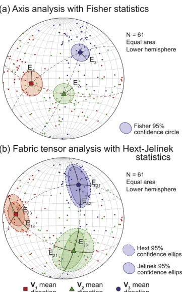
for statistical estimates of the distribution using Fisher statistics (Fisher, 1953) if data follows a unimodal distribution (one confidence angle; a circular confidence cone; Fig. 2a), and Bingham or Henry – Le Goff statistics (Bingham, 1964; Henry and Le Goff, 1995) if data distribution is bimodal (two confidence angles; an elliptical confidence cone). The main drawback of this approach is that the three principal directions of each ellipsoid are treated independently, whereas the orientation of each principal axis (e.g., V1) depends on the orientation of the other two axes (V2 and V3). The orthogonality of the resulting mean directions will not be preserved and the compiled lineations and foliations defined by an ellipsoid population are without meaning, notably in case of rela-tively scattered principal axes orientation (Fig. 2a).
2.2. Orientation tensor
The mean orientation tensor is a second-rank symmetric tensor constructed using the sum of the directional cosines of a single principal direction (e.g., V1). The method was developed in parallel by Schei-degger (1965) and Watson (1966). The orientation tensor is defined as: OVi¼ XN j¼1 ajaTj (2) with aj ¼ 0 @mljj nj 1
A, l, m, and n being the directional cosines of a specific principal direction (e.g., V1). Thus, OVi can be re-written as:
OVi¼ 2 6 6 6 4 X l2 Vi;j X lVi;jmVi;j X lVi;jnVi;j X mVi;jlVi;j X m2 Vi;j X mVi;jnVi;j X nVi;jlVi;j X nVi;jmVi;j X n2 Vi;j 3 7 7 7 5 (3)
OVi is frequently normalised by the sum of its eigenvalues or by the number of data points. The eigenvectors (v1, v2, v3) of the greatest, intermediate, and smallest eigenvalues (λ1, λ2, λ3) of O, corresponds to
axes with maximum, intermediate, and minimum strength, respectively. Similar to the axis analysis, OVi can only be calculated for an individual direction (e.g., OV1 for V1 axes) but the combination of orientation tensors cannot involve more than 2 principal directions (Lisle, 1989), simply because the sum of O from the three orthogonal directions is null. 2.3. Fabric tensor
Calculation of the three orthogonal principal axes and their inter-dependent level of confidence alone is not sufficient to fully quantify the fabric tensor because it requires combining information on the three principal axes into a single tensor. This can be done using a fabric tensor that can be described in a linear or quadratic form.
2.3.1. Linear fabric tensor
The linear fabric tensor corresponds to the sum of the three orien-tation tensors of characteristic axes multiplied by their lengths:
L ¼X N j¼1 � �V1;j � �aV1;jaTV1;jþ XN j¼1 � �V2;j � �aV2;jaTV2;jþ XN j¼1 � �V3;j � �aV3;jaTV3;j (4) with aV1;j ¼ 0 @mlV1;jV1;j nV1;j 1
A, l, m, and n being the directional cosines of a specific principal direction (here V1) and ||V1,j|| its length or norm. For example, the first element of equation (4) can be also written as: Fig. 2. Mean orientation statistics for the three principal axes defined by a set
of ellipsoids. (a) Axis analysis and associated Fisher statistics. E1, E2 and E3 are
cone half-opening angles for V1, V2 and V3 mean directions. (b) Fabric tensor analysis (linear fabric tensor) with Hext and Jelínek statistics. Hext-Jelínek confidence estimates result in elliptical confidence cones characterised by two half-opening angles (e.g., E13 and E12 for V1 in the direction of V3 and V1 in the
direction of V2, respectively). The red dashed line highlights the V1–V2 plane, i. e., the foliation defined by the SPO; the lineation corresponds to the direction of
V1. N: number of ellipsoids used for calculations. (For interpretation of the references to colour in this figure legend, the reader is referred to the Web version of this article.)
2.3.2. Quadratic fabric tensor
The quadratic fabric tensor design is identical to the fabric tensor based on the SLD method (Ketcham, 2005a; Odgaard et al., 1997; Smit and Odgaard, 1998), but it adopts only the three characteristic axes of individual ellipsoids: Q ¼X N j¼1 aV1;jaTV1;jþ XN j¼1 aV2;jaTV2;jþ XN j¼1 aV3;jaTV3;j (6) with aV1;j ¼ 0 @ � �V1;j��lV1;j � �V1;j��mV1;j � �V1;j��nV1;j 1
A, l, m, and n being the directional cosines of a specific principal direction (here V1) and ||V1,j|| its length. For example, the first element of Q, which is the fabric tensor of V1, can also be written as:
2.3.3. Fabric tensor analysis
Both the linear and the quadratic fabric tensors can be decomposed into eigenvectors (v1, v2, v3) of the greatest, intermediate, and smallest eigenvalues (λ1, λ2, λ3), which give the maximum, intermediate, and
minimum values of the “moment of inertia” i.e., the mean principal directions and lengths of V1, V2 and V3 of the fabric ellipsoid, which will be orthogonal (Fig. 2b). From the principal directions, the coordinates of the foliation and the lineation defined by the SPO of the ellipsoids can be calculated and correspond to the V1–V2 plane and to the V1 axis, respectively.
Several operations are applicable when constructing the orientation tensor. One consists of constructing the fabric tensor with normalised individual ellipsoid size (e.g., by the root of the sum of the square axis length or by the length of the V1 axis) so that all ellipsoids are weighted equally. This would avoid that the fabric tensor is dominated by a small number of highly anisotropic and large ellipsoids, which potentially form a secondary and weaker fabric (sub-fabric; see discussion below and in the work of Borradaile, 2001). For convenience, both L and Q can be normalised by the sum of its eigenvalues.
2.3.4. Confidence estimates
Calculations to estimate the data dispersion from second-rank ten-sors were initially proposed for anisotropy of magnetic susceptibility (AMS) measurements but are applicable to other second-rank tensors on the condition that they are symmetric. The methods permit calculation
of confidence angles that define an elliptical cone around each mean principal axis by integrating the mutually dependant distribution of the individual axes.
First, the Hext method (Hext, 1963; summarised in Tauxe, 2003) uses the mean value of the tensor diagonal elements and uses its devi-ation to calculate confidence angles. Three angles of confidence of the three mean directions are calculated: E12 ¼E21; E13 ¼E31; and E23 ¼E32, with E12 being the confidence angle around V1 in the direction of V2
(Fig. 2b), usually calculated at a 95% level of confidence.
The method of Jelínek (Jelínek, 1978; summarised in Tauxe, 2003) requires a larger number of calculations with the use of the covariance matrix of a reassembled tensor to construct three matrices whose ei-genvalues are used to derive six different confidence angles: E12, E21,
E13, E31, E23 and E32. Both methods usually provide similar confidence
angles, although the Hext method tends to generate larger confidence angles than those produced by the Jelínek method (Fig. 2b; Borradaile, 2003; Tauxe, 2003; Werner, 1997). Both Hext and Jelínek methods require measurements that have uncertainties with zero mean as well as
being normally distributed and small (see discussion in Tauxe, 2003). This can be verified using quantile-quantile plots (Q-Q plots; Tauxe, 2003). A third method was therefore developed by Constable and Tauxe (1990) using a bootstrapping approach that would be preferred in the presence of a sub-fabric (bimodal orientation distribution).
2.4. Fabric parameters
Second-order tensors are particularly appropriate to derive quanti-tative parameters characterising fabrics, as commonly done with structural data, EBSD or AMS. Indeed, fabric analysis can be performed either by using the eigenvalues of the orientation tensor of each axis treated separately (OVi; K-index; P, G, R values; parameters introduced below), a combination of eigenvalues of multiple orientation tensors (OV1 and OV3; LS-index) or simply the eigenvalues of the fabric tensor (L and Q; shape parameter T, corrected anisotropy P0). All parameters rely
on the following ellipsoid shape end-members: (1) Spherical ellipsoid if V1 ¼V2 ¼V3; (2) Planar ellipsoid if V1 ¼V2 >V3; (3) Linear ellipsoid if V1 >V2 ¼V3;
(4) Triaxial (neutral) ellipsoid if V1 >V2 >V3;
(5) The greater the difference between the lengths of each axis, the more anisotropic the ellipsoid becomes.
Most of these parameters can be calculated from a best fit ellipsoid (with V1, V2, V3 lengths) to each grain, but also for the fabric tensor XN j¼1 � �V1;j � �aV1;jaTV1;j¼ 2 6 6 6 6 4 X� �V1;j � �l2 V1;j X� �V1;j � �lV1;jmV1;j X� �V1;j � �lV1;jnV1;j X� �V1;j � �mV1;jlV1;j X� �V1;j � �m2 V1;j X� �V1;j � �mV1;jnV1;j X� �V1;j � �nV1;jlV1;j X� �V1;j � �nV1;jmV1;j X� �V1;j � �n2 V1;j 3 7 7 7 7 5 (5) XN j¼1 aV1;jaTV1;j¼ 2 6 6 6 6 6 4 X� �V1;j � �2 l2 V1;j X� �V1;j � �2 lV1;jmV1;j X� �V1;j � �2 lV1;jnV1;j X� �V1;j � �2 mV1;jlV1;j X� �V1;j � �2 m2 V1;j X� �V1;j � �2 mV1;jnV1;j X� �V1;j � �2 nV1;jlV1;j X� �V1;j � �2 nV1;jmV1;j X� �V1;j � �2 n2 V1;j 3 7 7 7 7 7 5 (7)
eigenvalues (λ1, λ2, λ3) resulting from the combination of many grains.
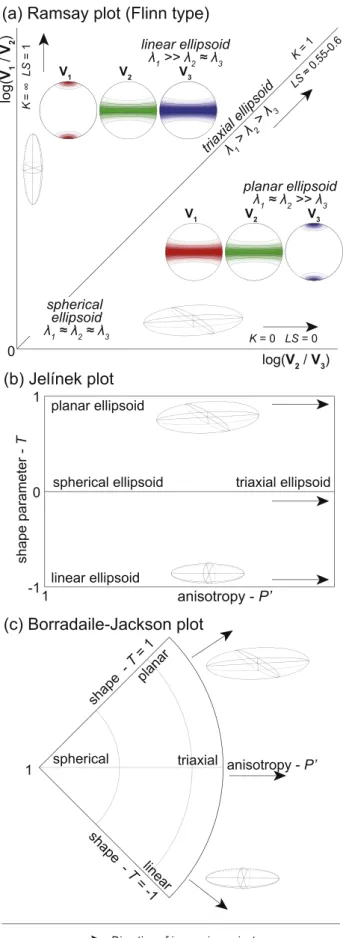
Various types of diagrams can be used to analyse the parameters calculated from each grain and from the fabric tensor (Fig. 3). 2.4.1. Shape parameters
One of the first parameters that was introduced is the K-index (Woodcock, 1977), which can be computed using any of the orientation tensors. It is most likely calculated using the orientation tensor of the longest axis of objects (i.e., c-axis for pyroxene, V1 for ellipsoids) and is defined by Woodcock, 1977 as:
K ¼lnðλ1=λ2Þ
lnðλ2=λ3Þ (8)
The K-index value ranges from 1 to ∞ for linear ellipsoids, approaches 1 for spherical and triaxial neutral ellipsoid and ranges from 1 to 0 for planar ellipsoids. It is an analogue to the Flinn (1962) or Ramsay (1967) diagram used in structural geology (Fig. 3a).
Alternatively, Vollmer (1990) proposed the definition of three pa-rameters to estimate the distribution of directions by the calculation of the P (equal 1 for point distribution), G (equal 1 for girdle distribution) and R (equal 1 for random distribution) parameters defined as follows:
P ¼ λ1 λ2;G ¼ 2 � ðλ2 λ3Þ;R ¼ 3 � λ3 (9)
with P þ G þ R ¼ 1 and λ1, λ2, and λ3 being the three eigenvalues of the
orientation tensor of the chosen principal axis.
The LS-index of Ulrich and Mainprice (2005) is constructed using the P, G, and R parameters of two perpendicular principal directions, commonly the largest and smallest axes (e.g., b- and c-axes of pyroxene,
V1 and V3 of ellipsoids, respectively), and are defined as: LS ¼1 2 � 2 � PV3 GV3þPV3 � � GV1 GV1þPV1 �� (10) with PV3 and GV3 being the P and G parameters calculated using the V3 orientation tensor and PV1 and GV1 being the P and G parameters calculated using the V1 orientation tensor. Consequently, the LS-index equals 1 for linear fabrics and is 0 for planar objects (Fig. 3a).
The shape parameter T, developed for AMS measurements, uses a tensor containing the information of the three orthogonal principal di-rections (i.e., a fabric tensor). It is defined by Jelínek (1981) as: T ¼lnðλ2=λ3Þ lnðλ1=λ2Þ
lnðλ2=λ3Þ þlnðλ1=λ2Þ (11)
The shape parameter T reflects shape of the fabric ellipsoid: rota-tional planar (1.0 � T > 0.5); planar to plano-linear (0.5 � T > 0.2); plano-linear (0.2 � T > 0.2); plano-linear to linear 0.2 � T > 0.5); rotational linear ( 0.5 � T � 1.0).
2.4.2. Anisotropy
The degree of anisotropy of the fabric can be inferred from the “corrected” anisotropy parameter P0(Jelínek, 1981) of the fabric tensor,
defined as: P’ ¼ exp ffiffiffiffiffiffiffiffiffiffiffiffiffiffiffiffiffiffiffiffiffiffiffiffiffiffiffiffiffiffiffiffiffiffiffiffiffiffiffiffiffiffiffiffiffiffiffiffiffiffiffiffiffiffiffiffiffiffiffiffiffiffiffiffiffiffiffiffiffiffiffiffiffiffiffiffiffiffiffiffiffiffiffiffiffiffiffiffiffiffiffiffiffi 2 �� ln � λ1 λm ��2 þ � ln � λ2 λm ��2 þ � ln � λ3 λm ��2� s (12) with λm ¼ ðλ1þ λ2þ λ3Þ=3. The P0 parameter increases from 1
(isotropic) up to values depending on the shape and distribution of its constituents. Both P0 and T parameters are combined to construct the
Jelínek plot, as particularly adapted for rock fabric analysis (Fig. 3b). However, low anisotropy ellipsoids that approach to a spherical shape can be graphically scattered in a standard Jelínek plot. To avoid this graphical bias, an alternative approach was proposed by Borradaile and Jackson (2010) with a polar P0-T plot (Fig. 3c).
Fig. 3. Examples of fabric diagrams, associated fabric ellipsoids and ideal
distribution of V1, V2 and V3 orientations. (a) Ramsay plot (modified Flinn diagram; Flinn, 1962; Ramsay, 1967), (b) standard P0-T plot (Jelínek plot;
Jelínek, 1981) and (c) polar P0-T plot (Borradaile and Jackson, 2010). Black
3. Implementation of the TomoFab program
The various methods for mean direction calculations, confidence ellipses and parameters informing about the characteristics of the fabric have been incorporated in the TomoFab MATLAB package (a continu-ously maintained version is available for download at https://github. com/benpetri/tomofab). The code runs on multiple platforms using MATLAB R2015a and newer versions without additional specific tool-boxes. The user can run the tomofab.m file, which launches promptly the graphical user interface or GUI (Fig. 4).
The GUI consists of different panels that allow loading and exporting data and plots and then visualizing and filtering input data using the ellipsoid volume. Input files are tab-separated value tables of ellipsoids and sample orientation information. Volume filtering automatically recalculates all statistical parameters and updates all plots. Orientation data are plotted in either equal area (Schmidt) or equal angle (Wülff) nets, however the equal area projection is recommended for fabric analysis to avoid the inherent density distortion of the stereographic equal angle projection. The user can identify data clustering (fabrics and sub-fabrics) using contoured density plots constructed with a modified Kamb method (Vollmer, 1995) displaying densities in 3σ (standard de-viation) or in multiples of uniform distribution (MUD).
Calculation of mean orientations can be performed either by vector analysis (orthogonality between the mean principal directions is not taken into account) or using the analysis of the fabric tensor (orthogo-nality between the mean principal directions is preserved). The user has the choice to either use a linear or a quadratic fabric tensor. Depending on the dataset, the user may normalise the size of each ellipsoid by the root of the sum of the squared axis lengths to limit the influence of a small number of large and highly anisotropic ellipsoids on the fabric tensor (the effect of the “sub-fabric” above described). Depending whether the orientation statistics were compiled by vector or tensor analysis, Fisher, Hext and Jelínek confidence cones can be calculated and displayed. Additional statistical methods can also be implemented such as Bingham statistics. For each loop of calculation, orientation parameters (mean V1, V2 and V3 direction, foliation, and lineation dip directions) are updated at the bottom-left of the window.
Fabric diagrams are updated at each calculation loop and consist of an ellipsoid aspect ratio (V1/V3) histogram, a PGR ternary diagram for each principal direction (Vollmer, 1990), a Ramsay plot using a log(||
V2||/||V3||) - log(||V1||/||V2||) correlation (Fig. 3a; modified from Flinn, 1962; Ramsay, 1967) and a Jelínek plot (P0-T; Fig. 3b; Jelínek, 1981) for individual ellipsoid but also for the fabric tensor. Alterna-tively, a polar P0-T plot of Borradaile and Jackson (2010) can be used,
with either a linear P0 axis or a log(P0) axis in case of dataset with
scattered individual ellipsoid P0, which is likely the case with geological
material analysed with μXCT compared to standard P0 values derived
from AMS dataset (usual P0values are ranging between 1 and 1.2).
All calculations can be performed in the sample coordinate system, but the full dataset can be re-oriented back to the geographic coordinate system. To do so, the sample orientation should be known and high-lighted by a physical mark before the tomography analysis, in order to apply upside down analysis, strike and dip angle corrections. In such a case, the program reads orientation information and applies corrections for each individual ellipsoid, and performs all calculations (axis or tensor analysis, confidence estimates, fabric parameters) in the geographic coordinate system.
4. Synthetic case study
In order to test the different methods of constructing fabric tensors and the implications for confidence ellipses calculation and fabric pa-rameters, we have generated synthetic datasets composed of ellipsoids with variable size, shape, and orientation distribution (Figs. 5–7). 4.1. Fabric parameters
The first dataset employed (Figs. 5 and 6) corresponds to a set of 50 planar and planar to plano-linear ellipsoids with V1 �1 mm, V2 �0.9 mm and V3 �0.6 mm and 3 linear to plano-linear ellipsoids with V1 �2 mm, V2 �0.9 mm and V3 �0.6 mm. These ellipsoids are rotated around their V1 axis to produce a linear fabric (Figs. 5a and 6a) or rotated around their V3 axis to produce a planar fabric (Figs. 5b and 6b). For better visibility, random noise is added to the orientation of the Fig. 4. Graphical user interface of TomoFab allowing to display, analyse and quantify orientation and fabric statistics.
Fig. 5. Synthetic datasets composed of ellipsoids with different orientation distribution illustrated with a 3D rendering of the ellipsoids, Schmidt net, PGR diagram,
Ramsay diagram, standard P0-T diagram and polar P0-T diagram. (a) Ellipsoids rotated around their V1 axes to produce a linear fabric. (b) Ellipsoids rotated around
their V3 axes to produce a planar fabric. The red dashed line highlights the V1–V2 plane, i.e., the foliation defined by the SPO; the lineation corresponds to the direction of V1. Statistics calculated with a linear fabric tensor and Hext confidence ellipses at 95% level of confidence. See text for details. Colour map from Crameri (2018) representing the distance to the ellipsoid centre. (For interpretation of the references to colour in this figure legend, the reader is referred to the Web version of this article.)
ellipsoids and the length of their axes.
The synthetic linear fabric (Fig. 5a) displays a point clustering of V1 axes and girdle distribution of V2 and V3 axes, confirmed by the PGR values and diagram. Accordingly, the use of a linear fabric tensor in-dicates V1 mean direction at V1 clustering point, whereas V2 and V3 mean directions lie on the girdle defined by V2 and V3 individual el-lipsoids axes. Compiled Hext confidence angles also highlight the V2–V3 girdle distribution, with E23 and E32 angles larger than the other angles.
The compiled fabric parameters (K ¼ 7.4; LS ¼ 0.87; T ¼ 0.50; P0¼1.5)
clearly indicate a linear to plano-linear fabric. It has to be noted that the shape parameter of the fabric ellipsoid has quite high values (T ¼ 0.5), despite the fact that high G values for V2 and V3 would rather lead to lower T values (T � 1). This is the result of the shape of the majority of the individual grains that are planar to plano-linear, avoiding extreme linear T values.
The synthetic planar fabric (Fig. 5b) displays a point clustering of V3 axes whereas V1 and V2 axes are distributed along a girdle, in agreement with the PGR values of the three principal axes. Using a linear fabric tensor, the mean V1 and V2 directions lie on the girdle defined by the individual ellipsoid principal axes, whereas mean V3 is located on the V3 cluster. The derived Hext confidence angles shows high opening values for E12 and E21 whereas the other confidence angles are rather small. In
agreement to this, the fabric parameters indicate a clearly planar fabric (K ¼ 0.06; LS ¼ 0.06; T ¼ 0.95; P0¼1.6). The shape parameter (T) is
quite high in comparison to the one compiled with the synthetic linear fabric (Fig. 5a) and is explained by the planar and planar to plano-linear shape of individual ellipsoids. This clearly demonstrates the influence of the shape of individual ellipsoids on the resulting fabric ellipsoid. 4.2. Linear vs. quadratic fabric tensor
Using the same two synthetic datasets, we have compiled mean orientation, confidence angles and fabric parameters from linear fabric tensors and quadratic fabric tensors (Fig. 6). The calculated mean principal axes for the synthetic linear fabric is almost identical between the two tensors. However, the mean principal directions of V1 and V2 for the synthetic planar fabric shows misorientation of ~10�but remains on
the girdle defined by the V1 and V2 individual ellipsoid orientations. The Hext confidence angles calculated using the two methods present sys-tematically smaller opening angles with a quadratic fabric tensor than with a linear fabric tensor. The fabric parameters that are derived from both linear (Fig. 6a; K ¼ 7.4; LS ¼ 0.87; T ¼ 0.53; P0¼2.2) and planar
synthetic fabrics (Fig. 6b; K ¼ 0.06; LS ¼ 0.06; T ¼ 0.92; P0¼2.9) still
indicates a plano-linear to linear fabric and a planar fabric, respectively. K- and LS- indexes are identical as they are compiled with V1 and V3 orientation tensors. This is not the case with the parameters derived from fabric tensors, notably for the anisotropy parameter P0: the squared
axes length favours long axes more than small axes when constructing Fig. 6. Difference in mean axes orientation, Hext confidence ellipses at 95% level of confidence and fabric statistics between linear fabric tensors and quadratic fabric
tensors compiled for the two datasets presented in Fig. 6: (a) synthetic linear fabric and (b) synthetic planar fabric. The red dashed line highlights the V1–V2 plane – i. e., the foliation defined by the SPO; the lineation corresponds to the direction of V1. (For interpretation of the references to colour in this figure legend, the reader is referred to the Web version of this article.)
the tensor, but also when deriving its eigenvalues and eigenvectors. This has several consequences: (1) the calculated mean principal directions with a quadratic fabric tensor are predominantly influenced by the orientation of the large ellipsoids compared to the small ellipsoids, explaining the misorientation of V1 and V2 observed in Fig. 6b; and (2) the quadratic fabric ellipsoid has a different shape parameter (T) value and higher degree of anisotropy (P0), which cannot be compared to
in-dividual ellipsoids.
4.3. Standardised fabric tensor
The second dataset employed (Fig. 7) is composed of 50 planar to plano-linear ellipsoids with V1 �1 mm, V2 �0.9 mm and V3 �0.6 mm and 3 larger linear ellipsoids with V1 �6 mm, V2 �0.9 mm and V3 � 0.6 mm. The axes orientation and length are varied slightly for better visualisation: the three large ellipsoids are defining a V1 cluster at 205/ 25 whereas the set of small ellipsoids are defining a V1 cluster at 260/20. As fabric tensors are constructed using the length of the character-istic axes of ellipsoids, more weight is attributed to large and highly anisotropic ellipsoids than to small and isotropic ellipsoids. The influ-ence of such outlier ellipsoids is moderate when using linear fabric tensors but dominant using quadratic fabric tensors. This effect is depicted in Fig. 7a, where the mean principal axes are lying in between the two clustering points, in particular for mean V1 and V3 axes. Con-fidence ellipses clearly show a triaxial fabric ellipsoid (note that the exemplified bimodal distribution might not be suitable for Hext and Jelínek confidence estimates; see section 2.3.4.). This is confirmed by the fabric statistics, especially by the T value (K ¼ 2.1; LS ¼ 0.50; T ¼
0.00; P0¼1.6). The mean axes orientation, the confidence ellipses and
the fabric statistics indicate that the three large ellipsoids define a sub- fabric that overcomes the fabric defined by the 50 smaller ellipsoids. This may occasionally lead to a decoupling between indexes derived from orientation tensors and indexes derived from fabric tensors (here K >1 and T ¼ 0). The sub-fabric effect is attenuated by normalising each individual ellipsoid by the root of the sum of the squared axes length to obtain “unit ellipsoids” (see details in Borradaile, 2001). In such a case, mean principal directions and fabric statistics are ruled by the most populated set of ellipsoids rather than by the largest and most aniso-tropic ellipsoids (Fig. 7b), which mean principal directions localised at individual axes clustering points, and confidence angles and fabric sta-tistics approaching values expected from the set of 50 small ellipsoids (K ¼2.1; LS ¼ 0.50; T ¼ 0.46; P0¼1.5).
5. Natural case study
The natural example represents a sub-volume of an oriented core (~45-mm diameter) collected with a portable rock drill (Fig. 8). It consists of a pyroxene-bearing gabbro from the exposed lower-crustal section of the Ivrea-Verbano Zone, in the gabbro-norite zone of the Upper Mafic Complex (sample MC07-02; 45.84826�N; 8.19640�E; Val
Mastallone, NW Italy). The sample is composed of pyroxenes, plagio-clase, and oxides (magnetite and ilmenite) and presents a well- developed foliation and lineation marked by the preferred orientation of magmatic pyroxene grains (Fig. 8a–c). Notably, the study of this sample allows a better understanding of the dynamics and the fabric development related to magma flow and emplacement in the lower Fig. 7. Influence of ellipsoid size and anisotropy on the linear fabric tensor analysis using datasets for which each individual ellipsoid is either (a) non-normalised or
(b) normalised by the root of the sum of the squared length (“unit ellipsoids”). The red dashed line highlights the V1–V2 plane – i.e., the foliation defined by the SPO; the lineation corresponds to the direction of V1. Hext confidence ellipses are plotted at 95% level of confidence. See text for details. Colour map from Crameri (2018)
representing the distance to the ellipsoid centre. (For interpretation of the references to colour in this figure legend, the reader is referred to the Web version of this article.)
crust.
The sample was imaged with a Bruker SkyScan 1173 X-ray micro- tomographer at the University of Lausanne (Switzerland) using a source voltage of 130 kV and a source current of 61 μA for 6 h, producing 801 slices with a 50 μm spatial resolution. Image segmentation and both automatic and manual separations (i.e., defining and isolating a set of connected voxels that constitutes a blob; see Appendix A for details) were performed using Blob3D (Ketcham, 2005b) before measuring each blob centre coordinates, volume and best-fit ellipsoid axis length and orientation using the same software. Figs. 9–10 present fabric and orientation distribution of pyroxene and oxide grains that were manu-ally separated and selected by their volume (0.5–8.5 mm3 for pyroxene;
0.1–2.4 mm3 for oxide). A comparison between automatic and manual
segmentation results is reported in Table 2 and as Supplementary Ma-terial (see Appendix A). In order to compare the results of our approach to state-of-the-art methods, we performed a Star Length Distribution (SLD) analysis using Quant3D (Ketcham, 2005a; Odgaard et al., 1997; Smit and Odgaard, 1998) on the same set of images segmented with Blob3D. The SLD is a continuum method of fabric characterization that does not require a separation of grains or even to consider grains, but suffers from being grain size sensitive; a large grain will be sampled and integrated several times, whereas smaller grains may even not be integrated.
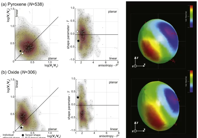
Individual best-fit ellipsoid of both pyroxene and oxide grains are scattered but pyroxene grains are preferentially plano-linear, whereas oxide grains are more elongated, being preferentially linear to plano- linear (Fig. 9). In the absence of solid-state deformation, these individ-ual grain shape parameters correspond to the almost ideal shape of magmatic pyroxenes and oxides.
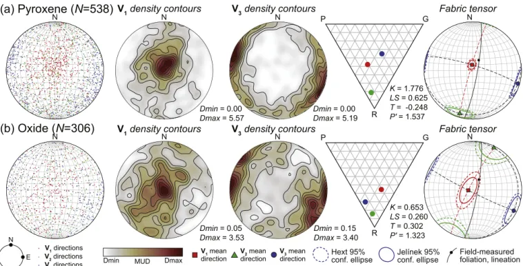
Orientation of individual grains best-fit ellipsoid of pyroxene grains (Fig. 10a) shows a clear V1 vertical point distribution with a weak vertical girdle that is striking towards the NNE. Conversely, V3 distri-bution presents a horizontal girdle distridistri-bution with ESE and WNW point maxima. The analysis of the linear fabric tensor compiled with the same dataset constrains a vertical foliation and a vertical lineation at
~10�from the field measured foliation and lineation. The fabric defined
by the pyroxene grains is linear to plano-linear as indicated by the analysis of the orientation tensors (K ¼ 1.776; LS ¼ 0.625) and the linear fabric tensor (T ¼ 0.248; P0¼1.537). The SLD analysis of segmented
but not separated images indicate a plano-linear fabric (Fig. 9a; λ1 ¼ 0.384; λ 2 ¼0.335; λ3 ¼0.281; equivalent to T ¼ 0.117 and P0¼1.367)
with higher equivalent T values than those ones derived from the linear fabric tensor, likely due to the integration of grains aggregates when using the SLD method.
The orientation distribution of oxide grains (Fig. 10b) is moderately scattered. The distribution of V1 orientations draws a moderately defined girdle that steeply dips to the ESE from which a vertical point distribution can be noticed. On the other hand, V3 distribution defines two ESE and WNW horizontal, but scattered, point distribution. The analysis of the linear fabric tensor presents rather similar orientations to those derived for the pyroxene grains, but with larger Hext and Jelínek confidence estimates due to the scattered distribution of individual grain orientation. Although oxide grains are individually quite elongated (Fig. 9b), the fabric they define is planar to plano-linear (K ¼ 0.653; LS ¼0.260; T ¼ 0.302; P0 ¼1.323). The results of both orientation and
fabric tensor analysis are in good agreement with the SLD analysis (Fig. 9b; λ1 ¼0.372; λ2 ¼0.342; λ3 ¼0.286; equivalent to T ¼ 0.351 and P0¼1.307).
In general, the use of automatically separated grains allows to give a first order constraint on the grain shape and fabric properties, but the analysis is disturbed by the integration of a large number of grain ag-gregates as well as randomly oriented, very small grains that are ruled out by volume filtering using TomoFab (see comparison in Appendix A). We have to highlight that in our example, both automatically and manually separated datasets lead to similar fabric properties which may not be the case for all datasets, notably in case of interconnected pores or grains (aggregates). However, manual separation clearly increases the quality of the dataset, allowing to better document the difference in fabric properties between the pyroxene and the oxide grain population that relates different stress regime during the sequential crystallisation Fig. 8.μXCT images and segmented images of a pyroxene-bearing gabbro from the Upper Mafic Complex in the Ivrea-Verbano Zone (Southern Alps, North Italy). (a) Section of the core showing the physical mark needed to reorient data to the geographical reference frame. (b) Reconstructed volume showing the analysed sample and the physical mark. (c) Reconstructed section across the analysed core showing coarse grained pyroxene, plagioclase and oxide gabbro with a well-developed magmatic foliation. Segmented sub-volume presenting (d) pyroxene and (e) oxide blobs processed with Blob3D (Ketcham, 2005b), represented in the sample reference frame. Px: pyroxenes; Pl: plagioclase; Op: opaque mineral (oxides; magnetite and ilmenite).
Fig. 9. Fabric diagrams of segmented and manually separated pyroxene (0.5–8.5 mm3) and oxide (0.1–2.4 mm3) grains of Fig. 8de simplified to best-fit ellipsoids.
The black filled tensor shape parameters reported in the Ramsay and Jelínek plots derive from the compiled linear fabric tensor, the white filled tensor shape parameters derive from the SLD fabric tensor. Rightmost images are star length distribution diagrams calculated on Blob3D-segmented images using Quant3D (Ketcham, 2005a) in sample reference frame. N: number of ellipsoids used for calculations. Density colour map from Crameri (2018). (For interpretation of the references to colour in this figure legend, the reader is referred to the Web version of this article.)
of the various mineralogical phases (Table 2). Notably, the oxide grain population, although being linear to plano-linear in general, the fabric they define is planar to plano-linear showing that they behave as passive markers of the deformation – i.e., individual grain shape does not always translate deformation regimes.
6. Conclusion
We have designed and constructed a versatile fabric tensor analysis tool to characterise rock fabrics using segmented micro-computed to-mography datasets. We defined the linear fabric tensor and the quadratic fabric tensor using the sum of the orientation tensors of the three characteristic axes of grains (simplified to best fit ellipsoids) multiplied by the length or squared length of each axis, respectively. The use of the fabric tensor allows calculation of three orthogonal mean principal axes, their elliptical cones of confidence and the two main parameters relevant to rock fabric quantitative characterisation: the fabric ellipsoid shape and the degree of anisotropy. This approach is implemented in TomoFab, an open-source MATLAB package that is
freely available for download. The method permits quantitative com-parison of rock fabrics of different samples imaged by micro-computed tomography, but also to fabrics constrained by other independent methods (EBSD, AMS, and seismic anisotropy). The examples described above demonstrate the wide applicability of the method. Ultimately, the software can be more broadly used in Earth and material sciences and, potentially, in other fields when considering analyses of material fabrics and porosity.
7. Computer code availability
TomoFab is an open source MATLAB package available for download at https://github.com/benpetri/tomofab. TomoFab is developed under a GNU licence by Benoît PETRI (see corresponding author information). The code runs on multiple platforms using MATLAB R2015a and newer versions without additional specific toolboxes.
Fig. 10. Orientation distribution of segmented and manually separated (a) pyroxene (0.5–8.5 mm3) and (b) oxide (0.1–2.4 mm3) grains simplified to best-fit
el-lipsoids. Raw ellipsoids V1 and V3 orientation densities are represented in multiples of uniform distribution (MUD), analysed and contoured using TomoFab. Orientation data (equal area lower hemisphere spherical projection) are in the geographic reference frame. The red dashed line highlights the V1–V2 plane, i.e., the foliation defined by the SPO; the lineation corresponds to the direction of V1. Statistics performed with a linear fabric tensor and both Hext (dashed) and Jelínek (solid) confidence estimates at 95% level of confidence. N: number of ellipsoids used for calculations. The solid black line and point reports the field-measured foliation and lineation. Density colour map from Crameri (2018). (For interpretation of the references to colour in this figure legend, the reader is referred to the Web version of this article.)
Table 2
Summary of fabric parameters and orientation derived from the analysis of linear fabric tensors constructed using manually or automatically separated blobs. See
Figs. 9–10 and Appendix A for related diagrams.
Separation N K LS T P0 Foliation Lineation
Pyroxene manual 538 1.776 0.625 0.248 1.537 286/86 352/80 automatic 658 1.209 0.526 0.103 1.468 287/86 342/83 Oxide manual 306 0.653 0.260 0.302 1.323 297/83 267/82 automatic 260 0.798 0.275 0.108 1.400 301/82 301/82
Declaration of competing interest
The authors declare that they have no known competing financial interests or personal relationships that could have appeared to influence the work reported in this paper.
Acknowledgments
This work was supported by the University of Lausanne and the University of Strasbourg and by an ExxonMobil research grant to BP. BA received funding for this project from the Swedish Research Council grant 2018–03414. MP acknowledges the Ambizione Fellowship (PZOOP2_168166), supported by the Swiss National Science Founda-tion, for fieldwork and rock sampling in the Ivrea-Verbano Zone (Italy) and rock analysis by μXCT at UNIL. Pauline Le Maire is thanked for fruitful discussions around orientation data treatment and MATLAB programming. Lukas P. Baumgartner and Benita Putlitz are gratefully thanked for giving access to the UNIL μXCT facility as well as Othmar Müntener for insightful discussions. We thank Frederick W. Vollmer, the two anonymous reviewers, as well as the Editor-in-chief Dario Grana and the Associate Editor Eileen Martin for their helpful comments and editorial handling.
Appendix A. Supplementary data
Supplementary data to this article can be found online at https://doi. org/10.1016/j.cageo.2020.104444.
References
Bascou, J., Barruol, G., Vauchez, A., Mainprice, D., Egyrio-Silva, M., 2001. EBSD- measured lattice-preferred orientations and seismic properties of eclogites. Tectonophysics 342, 61–80.
Benn, D.I., 1994. Fabric shape and the interpretation of sedimentary fabric data. SEPM J. Sediment. Res. 64A https://doi.org/10.1306/D4267F05-2B26-11D7-
8648000102C1865D.
Benn, K., Allard, B., 1989. Preferred mineral orientations related to magmatic flow in ophiolite layered gabbros. J. Petrol. 30, 925–946.
Bingham, C., 1964. Distributions on the Sphere and on the Projective Plane. PhD Thesis. Yale University.
Borradaile, G.J., 2003. Statistics of Earth Science Data: Their Distribution in Time, Space and Orientation. Springer Science & Business Media.
Borradaile, G.J., 2001. Magnetic fabrics and petrofabrics: their orientation distributions and anisotropies. J. Struct. Geol. 23, 1581–1596. https://doi.org/10.1016/S0191- 8141(01)00019-0.
Borradaile, G.J., Jackson, J.A., 2010. Structural geology, petrofabrics and magnetic fabrics (AMS, AARM, AIRM). J. Struct. Geol. 32, 1519–1551.
Bryon, D.N., Atherton, M.P., Hunter, R.H., 1995. The interpretation of granitic textures from serial thin sectioning, image analysis and three-dimensional reconstruction. Mineral. Mag. 59, 203–211. https://doi.org/10.1180/minmag.1995.059.395.05. Chopin, F., Schulmann, K., �Stípsk�a, P., Martelat, J.E.E., Pitra, P., Lexa, O., Petri, B., 2012.
Microstructural and metamorphic evolution of a high-pressure granitic orthogneiss during continental subduction (Orlica-�Snie_znik dome, Bohemian Massif). J. Metamorph. Geol. 30, 347–376. https://doi.org/10.1111/j.1525- 1314.2011.00970.x.
Constable, C., Tauxe, L., 1990. The bootstrap for magnetic susceptibility tensors. J. Geophys. Res. 95, 8383. https://doi.org/10.1029/JB095iB06p08383. Crameri, F., 2018. Scientific colour-maps. Zenodo. https://doi.org/10.5281/
zenodo.1243862.
Fisher, N.I., Lewis, T., Embleton, B.J.J., 1993. Statistical Analysis of Spherical Data. Cambridge university press.
Fisher, R., 1953. Dispersion on a sphere. Proc. R. Soc. A Math. Phys. Eng. Sci. 217, 295–305. https://doi.org/10.1098/rspa.1953.0064.
Flinn, D., 1962. On folding during three-dimensional progressive deformation. Q. J. Geol. Soc. 118, 385–428. https://doi.org/10.1144/gsjgs.118.1.0385. Harrigan, T.P., Mann, R.W., 1984. Characterization of microstructural anisotropy in
orthotropic materials using a second rank tensor. J. Mater. Sci. 19, 761–767. https:// doi.org/10.1007/BF00540446.
Heilbronner, R.P., 1992. The autocorrelation function: an image processing tool for fabric analysis. Tectonophysics 212, 351–370. https://doi.org/10.1016/0040-1951 (92)90300-U.
Henry, B., Le Goff, M., 1995. Application de l’extension bivariate de la statistique Fisher aux donn�ees d’anisotropie de susceptibilit�e magn�etique: int�egration des incertitudes de mesure sur l’orientation des directions principales. Comptes rendus l’Acad�emie des Sci. S�erie 2. Sci. la terre des plan�etes 320, 1037–1042.
Hext, G.R., 1963. The estimation of second-order tensors, with related tests and designs. Biometrika 50, 353–373. https://doi.org/10.2307/2333905.
Higgins, M.D., 2006. Quantitative Textural Measurements in Igneous and Metamorphic Petrology. Cambridge University Press, Cambridge. https://doi.org/10.1017/ CBO9780511535574.
Hirt, A.M., Almqvist, B.S.G., 2012. Unraveling magnetic fabrics. Int. J. Earth Sci. 101, 613–624. https://doi.org/10.1007/s00531-011-0664-0.
Islam, A., Chevalier, S., Sassi, M., 2018. Structural characterization and numerical simulations of flow properties of standard and reservoir carbonate rocks using micro- tomography. Comput. Geosci. 113, 14–22. https://doi.org/10.1016/j.
cageo.2018.01.008.
Jelínek, V., 1981. Characterization of the magnetic fabric of rocks. Tectonophysics 79, T63–T67. https://doi.org/10.1016/0040-1951(81)90110-4.
Jelínek, V., 1978. Statistical processing of anisotropy of magnetic susceptibility measured on groups of specimens. Studia Geophys. Geod. 22, 50–62. https://doi. org/10.1007/BF01613632.
Jerram, D.A., Higgins, M.D., 2007. 3D analysis of rock textures: quantifying igneous microstructures. Elements 3, 239–245.
Ketcham, R.A., 2005a. Three-dimensional grain fabric measurements using high- resolution X-ray computed tomography. J. Struct. Geol. 27, 1217–1228. https://doi. org/10.1016/j.jsg.2005.02.006.
Ketcham, R.A., 2005b. Computational methods for quantitative analysis of three- dimensional features in geological specimens. Geosphere 1, 32–41. https://doi.org/ 10.1130/GES00001.1.
Ketcham, R.A., Carlson, W.D., 2001. Acquisition, optimization and interpretation of X- ray computed tomographic imagery: applications to the geosciences. Comput. Geosci. 27, 381–400. https://doi.org/10.1016/S0098-3004(00)00116-3. Launeau, P., Cruden, A.R., 1998. Magmatic fabric acquisition mechanisms in a syenite:
results of a combined anisotropy of magnetic susceptibility and image analysis study. J. Geophys. Res. Solid Earth 103, 5067–5089. https://doi.org/10.1029/97JB02670. Launeau, P., Robin, P.-Y.F., 2005. Determination of fabric and strain ellipsoids from
measured sectional ellipses—implementation and applications. J. Struct. Geol. 27, 2223–2233. https://doi.org/10.1016/j.jsg.2005.08.003.
Launeau, P., Robin, P.-Y.F., 1996. Fabric analysis using the intercept method. Tectonophysics 267, 91–119. https://doi.org/10.1016/S0040-1951(96)00091-1.
Lisle, R.J., 1989. The statistical analysis of orthogonal orientation data. J. Geol. 97, 360–364.
Macente, A., Fusseis, F., Menegon, L., Xiao, X., John, T., 2017. The strain-dependent spatial evolution of garnet in a high- P ductile shear zone from the Western Gneiss Region (Norway): a synchrotron X-ray microtomography study. J. Metamorph. Geol. 35, 565–583. https://doi.org/10.1111/jmg.12245.
Mardia, K.V., Jupp, P.E., 2009. Directional Statistics. John Wiley & Sons.
Moreno Ch�avez, G., Castillo Rivera, F., Sarocchi, D., Borselli, L., Rodríguez-Sedano, L.A., 2018. FabricS: a user-friendly, complete and robust software for particle shape-fabric analysis. Comput. Geosci. 115, 20–30. https://doi.org/10.1016/j.
cageo.2018.02.005.
Nicolas, A., 1992. Kinematics in magmatic rocks with special reference to gabbros. J. Petrol. 33, 891–915. https://doi.org/10.1093/petrology/33.4.891.
Odgaard, A., 1997. Three-dimensional methods for quantification of cancellous bone architecture. Bone 20, 315–328. https://doi.org/10.1016/S8756-3282(97)00007-0. Odgaard, A., Kabel, J., van Rietbergen, B., Dalstra, M., Huiskes, R., 1997. Fabric and
elastic principal directions of cancellous bone are closely related. J. Biomech. 30, 487–495. https://doi.org/10.1016/S0021-9290(96)00177-7.
Petri, B., Skrzypek, E., Mohn, G., Mateeva, T., Robion, P., Schulmann, K., Manatschal, G., Müntener, O., 2018. Mechanical anisotropies and mechanisms of mafic magma ascent in the middle continental crust: the Sondalo magmatic system (N Italy). GSA Bull 130, 331–352. https://doi.org/10.1130/B31693.1.
Prior, D.J., Boyle, A.P., Brenker, F., Cheadle, M.C., Day, A., Lopez, G., Peruzzo, L., Potts, G.J., Reddy, S., ans Nick, E., Timms, R.S., Trimby, P., Wheeler, J., Zetterstr€om, L., 1999. The application of electron backscatter diffraction and orientation contrast imaging in the SEM to textural problems in rocks. Am. Mineral. 84, 1741–1759.
Ramsay, J.G., 1967. Folding and Fracturing of Rock. McGraw-Hill, New York. Robin, P.-Y.F., 2002. Determination of fabric and strain ellipsoids from measured
sectional ellipses — theory. J. Struct. Geol. 24, 531–544. https://doi.org/10.1016/ S0191-8141(01)00081-5.
Scheidegger, A.E., 1965. On the statistics of the orientation of bedding planes, grain axes, and similar sedimentological data. U. S. Geol. Surv. Prof. Pap. 525, 164–167. Sch€opa, A., Floess, D., de Saint Blanquat, M., Annen, C., Launeau, P., 2015. The relation
between magnetite and silicate fabric in granitoids of the Adamello Batholith. Tectonophysics 642, 1–15. https://doi.org/10.1016/j.tecto.2014.11.022. Shan, Y., 2008. An analytical approach for determining strain ellipsoids from
measurements on planar surfaces. J. Struct. Geol. 30, 539–546. https://doi.org/ 10.1016/j.jsg.2006.12.004.
Smit, Schneider, Odgaard, 1998. Star length distribution: a volume-based concept for the characterization of structural anisotropy. J. Microsc. 191, 249–257. https://doi.org/ 10.1046/j.1365-2818.1998.00394.x.
Som, S.M., Hagadorn, J.W., Thelen, W.A., Gillespie, A.R., Catling, D.C., Buick, R., 2013. Quantitative discrimination between geological materials with variable density contrast by high resolution X-ray computed tomography: an example using amygdule size-distribution in ancient lava flows. Comput. Geosci. 54, 231–238.
https://doi.org/10.1016/j.cageo.2012.11.019.
Starnoni, M., Pokrajac, D., Neilson, J.E., 2017. Computation of fluid flow and pore-space properties estimation on micro-CT images of rock samples. Comput. Geosci. 106, 118–129. https://doi.org/10.1016/j.cageo.2017.06.009.
Tauxe, L., 2003. Paleomagnetic Principles and Practice, Modern Approaches in Geophysics. Kluwer Academic Publishers, Dordrecht. https://doi.org/10.1007/0- 306-48128-6.
Titschack, J., Baum, D., Matsuyama, K., Boos, K., F€arber, C., Kahl, W.-A., Ehrig, K., Meinel, D., Soriano, C., Stock, S.R., 2018. Ambient occlusion – a powerful algorithm to segment shell and skeletal intrapores in computed tomography data. Comput. Geosci. 115, 75–87. https://doi.org/10.1016/j.cageo.2018.03.007.
Ulrich, S., Mainprice, D., 2005. Does cation ordering in omphacite influence development of lattice-preferred orientation? J. Struct. Geol. 27, 419–431. https:// doi.org/10.1016/j.jsg.2004.11.003.
Vollmer, F.W., 1995. C program for automatic contouring of spherical orientation data using a modified Kamb method. Comput. Geosci. 21, 31–49. https://doi.org/ 10.1016/0098-3004(94)00058-3.
Vollmer, F.W., 1990. An application of eigenvalue methods to structural domain analysis. Geol. Soc. Am. Bull. 102, 786–791.
Vontobel, P., Lehmann, E.H., Hassanein, R., Frei, G., 2006. Neutron tomography: method and applications. Phys. B Condens. Matter 385–386, 475–480. https://doi.org/ 10.1016/j.physb.2006.05.252.
Watson, G.S., 1966. The statistics of orientation data. J. Geol. 74, 786–797. Watson, G.S., Irving, E., 1957. Statistical methods in rock magnetism. Geophys. J. Int. 7,
289–300. https://doi.org/10.1111/j.1365-246X.1957.tb02882.x. Werner, T., 1997. Experimental designs for determination of the anisotropy of
remanence-test of the efficiency of least-square and bootstrap methods applied to metamorohic rocks from southern Poland. Phys. Chem. Earth 22, 131–136. https:// doi.org/10.1016/S0079-1946(97)00090-6.
Whitehouse, W.J., 1974. The quantitative morphology of anisotropic trabecular bone. J. Microsc. 101, 153–168. https://doi.org/10.1111/j.1365-2818.1974.tb03878.x. Woodcock, N.H., 1977. Specification of fabric shapes using an eigenvalue method. Geol.
Soc. Am. Bull. 88, 1231. https://doi.org/10.1130/0016-7606(1977)88<1231: SOFSUA>2.0.CO;2.