Modeling of trace gases from the 1998 North Central Mexico forest fire smoke plume, as measured over Phoenix

(1)

HAL Id: hal-00301206

https://hal.archives-ouvertes.fr/hal-00301206

Submitted on 18 Apr 2006

HAL is a multi-disciplinary open access

archive for the deposit and dissemination of sci-entific research documents, whether they are pub-lished or not. The documents may come from teaching and research institutions in France or abroad, or from public or private research centers.

L’archive ouverte pluridisciplinaire HAL, est destinée au dépôt et à la diffusion de documents scientifiques de niveau recherche, publiés ou non, émanant des établissements d’enseignement et de recherche français ou étrangers, des laboratoires publics ou privés.

Modeling of trace gases from the 1998 North Central

Mexico forest fire smoke plume, as measured over

Phoenix

V. R. Kotamarthi, P. V. Doskey, S. R. Springston, P. Hyde, J. S. Gaffney, N.

A. Marley

To cite this version:

V. R. Kotamarthi, P. V. Doskey, S. R. Springston, P. Hyde, J. S. Gaffney, et al.. Modeling of trace gases from the 1998 North Central Mexico forest fire smoke plume, as measured over Phoenix. Atmospheric Chemistry and Physics Discussions, European Geosciences Union, 2006, 6 (2), pp.3227-3264. �hal-00301206�

(2)

ACPD

6, 3227–3264, 2006

Forest fire smoke plume V. R. Kotamarthi et al. Title Page Abstract Introduction Conclusions References Tables Figures J I J I Back Close

Full Screen / Esc

Printer-friendly Version Interactive Discussion

EGU

Atmos. Chem. Phys. Discuss., 6, 3227–3264, 2006 www.atmos-chem-phys-discuss.net/6/3227/2006/ © Author(s) 2006. This work is licensed

under a Creative Commons License.

Atmospheric Chemistry and Physics Discussions

Modeling of trace gases from the 1998

North Central Mexico forest fire smoke

plume, as measured over Phoenix

V. R. Kotamarthi1, P. V. Doskey1, S. R. Springston2, P. Hyde3, J. S. Gaffney1, and N. A. Marley1

1

Environmental Science, Argonne National Laboratory, 9700 South Cass Avenue, Argonne, IL 60439-4843, USA

2

Brookhaven National Laboratory, Upton, NY, USA

3

Arizona Department of Environmental Quality, Phoenix, AZ, USA

Received: 16 January 2006 – Accepted: 10 February 2006 – Published: 18 April 2006 Correspondence to: V. R. Kotamarthi (vrkotamarthi@anl.gov)

(3)

ACPD

6, 3227–3264, 2006

Full Screen / Esc

EGU

Abstract

Forest fires in North and Central America have been frequent and extensive over the past few years. Though much research has addressed the effects of forest fires in tropical South America and Africa on regional and global-scale oxidants, the same is not true for North America. Here we show that one of the days during an intensive field

5

campaign conducted over Phoenix, Arizona, in 1998 was substantially influenced by transport from forest fires in central and southern Mexico. We combined data collected from aircraft platforms, surface stations, and satellite with model results to establish that the origin of the air sampled over Phoenix on 20 May 1998, was from forest fires in Mexico. We also investigated the effect of the smoke layer on photolysis rates and

10

hence photochemistry over a five-day travel period from the source region to Phoenix. The results show that a smoke layer could reduce photolysis rates of key tropospheric constituents significantly and decrease the oxidant formation rates during the first few days of the plume history. The ultimate effect of the smoke layer on the evolution of oxidants in the plume was, however, shown to be minimal.

15

1 Introduction

Biomass burning emissions profoundly affect air quality on local scales. The deterio-ration of air quality due to smoke includes reduced visibility and increases in CO and hydrocarbon mixing ratios in the immediate vicinity. These conditions can last several weeks to months, depending on the duration of the event. Biomass burning resulting

20

from both anthropogenic activities (e.g., forest clearing, activities associated with agri-culture) and natural events (e.g., lightning strikes in drought conditions) affects forested areas. Much attention has been focused on potential effects of large-scale events such as the massive burning of tropical rain forests (Fishman et al., 1991; Longo et al., 1999; Thompson et al., 2001). However, little is known about the short-term effects

25

(4)

ar-ACPD

6, 3227–3264, 2006

Full Screen / Esc

EGU

eas (Wong and Li, 2002). The impact of such forest fires on ozone mixing ratios near the surface and throughout the tropospheric column over North America needs further investigation.

We had an opportunity, during the year 1998 over Phoenix, Arizona, to sample air impacted by forest fires in North Central Mexico. The measurements were part of an

5

intensive six-week study conducted in May and June, in and around Phoenix, as a part of a U.S. Department of Energy (DOE) Atmospheric Chemistry Program initiative in collaboration with the Arizona Department of Environmental Quality (ADEQ). Mea-surements of meteorological variables were made during this campaign to improve simulations of the flow conditions in the region (Fast et al., 2001). Meanwhile, an

ex-10

haustive characterization of the chemical composition of the air was conducted from a small aircraft (Gulfstream G-1). Argonne ground-based monitoring stations augmented those operated by the ADEQ (Gaffney et al., 2002; Doskey et al., 2000).

Extensive forest fires reported in central and northern Mexico during April and May of 1998 covered thousands of acres (Peppler et al., 2000). The plume from these fires

15

reached as far north as Wisconsin. Ground-based measurements of the optical char-acteristics of the smoke plume were reported from the DOE Atmospheric Radiation Measurement Program’s Southern Great Plains (SGP) site in Oklahoma, as well as in Texas and other southwestern U.S. states. Peppler et al. (2000) reported an increase in ozone and mixing ratios above 80 ppb on 7, 12, 13, 15, 19, 20, and 22 May at the

20

SGP site. They also observed increase in large particles (sizes greater than 10 nm) in the atmosphere on 5, 8, 12, 16, 24, and 25 May. Aerosol single scattering albedos were highest on 10, 14, and 18 May. It is difficult to attribute the increase in ozone at this location to the smoke event. Rather, the general southerly direction of the wind flow during this period is thought to have contributed to the observed ozone, because

sev-25

eral highly polluted urban areas in Texas are directly south of the SGP site. During May and June 1998, thousands of acres of biomass are estimated to have burned. Here we focus on a set of trace gas measurements made during the Phoenix 1998 experiment that show the presence of the plume over Phoenix and provide some indications of its

(5)

ACPD

6, 3227–3264, 2006

Full Screen / Esc

EGU

effect on atmospheric chemistry on the regional scale.

Figures 1a and b show the aerosol optical depth obtained from the TOMS (Total Ozone Mapping Spectrometer) satellite instrument for 19 and 20 May (Torres et al., 2002). Smoke aerosols, composed mainly of soot particles, are expected to absorb radiation and thus give positive values for aerosol optical depth. Such values (>0) are

5

evident approaching the Phoenix area on 19 May (Fig. 1a) but are less prominent on 20 May (Fig. 1b). The TOMS data resolution is 1.25◦ longitude by 1.0◦ latitude (a square grid approximately 100 km by 80 km), and the local overpass time for the Phoenix area is around noon daily.

The aerosol index values <1 that appear frequently in the data files do not

neces-10

sarily represent smoke aerosols. However, in this particular case, evidence from other measurements made in and around Phoenix supports the assertion that these obser-vations do represent smoke aerosols. The contours with aerosol index >2.5 in western and southern Mexico are close to the regions identified as the source of the forest fires in various media reports.

15

Measurements made on 20 May at the Usery Pass surface site, to the southwest of the Phoenix urban area, will be analyzed together with the measurements made from the G-1 aircraft on 21 May and 22 May over the Phoenix urban air shed for indications of the forest fire plume and its net effect on the atmospheric chemistry of this region. In addition, measurements made by the ADEQ at its Central Phoenix site, also known

20

as the Phoenix Supersite site, will be used to supplement our data and support our conclusions.

2 Measurements over Phoenix of the North Central Mexico forest fire plume

The measurements made in Phoenix during May–June of 1998 were part of a field campaign conducted by the DOE Atmospheric Chemistry Program. Surface-level

mea-25

surements of NO_x, NO, NO₂, ozone, CO, and several hydrocarbons were made at a surface site at Usury Pass, 30 km from the center of the Phoenix. Measurements were

(6)

ACPD

6, 3227–3264, 2006

Full Screen / Esc

EGU

also made from the G-1 aircraft on several of the days. A complete description of the flight plans, mission objectives, and data is online (http://www.Atmos.anl.gov/ACP). The NO_x, CO, and ozone measurements made at the surface station were reported by Gaffney et al. (2002). The focus here is on two days in May 1998 when aircraft and surface observations of a host of gas-phase chemical tracers were made in and around

5

Phoenix.

20 May was marked by low ozone (30–40 ppbv), high CH₃Cl (∼900 pptv), and low NO_xat the Usery pass site (Gaffney et al., 2002). The Central Phoenix site, located in downtown Phoenix and operated by the ADEQ, also showed remarkable differences on 20 May versus the other days. Figure 2a shows an average ozone level for a period of

10

approximately four weeks, from 15 May to 12 June, with the diurnal profile for 20 May for comparison. The ozone level for 20 May was less than half of the average value for the corresponding time period during the afternoon peak ozone hours. The diurnal profile on 20 May also showed a flatter, broader peak during the daytime, uncharacteristic of a urban source dominated by locally produced ozone. This observation suggests that

15

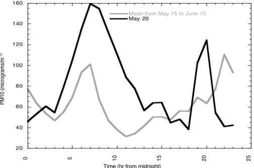
the ozone on 20 May originated mostly from long-range transport. This day also had a higher-than-average (by about 50%) CO level (Fig. 2b), compared to the four-week period defined above. Similar behavior was also shown by the measured PM10 at the Central Phoenix site (Fig. 2c). Interestingly, an appreciable increase in NO_x was also measured by the ADEQ. This additional NO_x mostly likely resulted from lower rates of

20

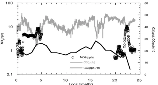
conversion of NO_x to HNO₃ in the air as a result of decreased photochemical activity in the smoky conditions. Measurements made away from the city, at the Usery Pass site (Gaffney et al., 2002), show similar low ozone values. The ozone level reported at the Usery Pass site for 20 May (∼40 ppbv) was among the lowest values for the month of May (Fig. 3). The ultraviolet light (UV) recorded on this day was also lower by about

25

30–50% than on the previous day (data not shown).

Measurements were also made from the G-1 aircraft on 21 May and 22 May. Unfor-tunately, no measurements were made from this aircraft platform on 20 May because of poor visibility. However, even on 21 May, the air above the boundary layer was

(7)

ACPD

6, 3227–3264, 2006

Full Screen / Esc

EGU

substantially impacted by long-range transport from the forest fires. Figure 4a shows measured ozone from the aircraft platform as a function of altitude and time (GMT). The aircraft climbed from an altitude of 500 m after takeoff to an altitude of over 3000 m on both days and then spiraled down to approximately 1000 m. We focus our attention on this level leg of the flight, extending from approximately 60 000 seconds GMT (local

5

time ∼08:20 a.m.) to 62 000 s GMT (∼09:15 a.m.). Measured ozone at approximately the same altitude was lower by almost 20 ppbv on 21 May than on 22 May. The water vapor mixing ratios for these two days differed by a factor of 2–3 (Fig. 4b). The mix-ing ratios for methyl hydrogen peroxide (Fig. 4c) and hydrogen peroxide (Fig. 4d) were similarly different by factors of 2–3. Lee et al. (1997) reported that biomass burning

10

plumes are generally accompanied by an increase in the mixing ratios of these perox-ide compounds. These observations would indicate that the air mass sampled on 21 May from the aircraft platform originated from biomass burning.

In the rest of the discussion, we establish the origin of the air mass by using air-parcel trajectory calculations, then use model calculations to determine the reasons for

15

the low ozone levels in the plume observed over Phoenix on 20 May 1998.

3 Model calculations

Back trajectories from Phoenix were calculated for the month of May 1998 to investigate the origin of the air mass sampled during the field experiment. The calculations were performed mainly to examine the smoke event observed on 20 May over Phoenix. A

20

well-established mesoscale meteorological model (MM5 V.3) was used to generate meteorological fields on fine spatial and time scales for a 20-day period from 10 May to 30 May. The model had a grid resolution of approximately 90 km by 90 km and extended from 5◦ to 42◦N latitude and from 130◦ to 80◦W longitude. The 23 vertical levels in the model had vertical resolution ranging from 50 m near the surface to more

25

than 2 km at the model top, situated at 100 mb. The mesoscale meteorological model was initialized by using NCEP (National Centers for Environmental Protection) 4-D

(8)

ACPD

6, 3227–3264, 2006

Full Screen / Esc

EGU

(four-dimensional) reanalysis (version 1) data for May 1998 obtained from the National Center for Atmospheric Research. The NCEP 4-D reanalysis data set was also used to derive the model boundary conditions for the simulation period. Output fields from the model were saved every hour for the 20 days from 10 May to 30 May.

Back trajectories based on the calculated wind velocities from the model, usually

5

referred to as kinematic trajectories, were calculated for each day from 15 May to 25 May. The results were then plotted in groups of trajectories, with those originating at 850 mb and below as one set. Mid-troposphere trajectories extending from 850 mb to 500 mb were plotted as the second set, those from 500 mb to 300 mb as the third set. Figure 5 shows the results for air parcels reaching Phoenix on 20 May at approximately

10

08:00 a.m. The figure shows that for this set of trajectories, the air parcels in the at-mospheric boundary layer originated in western Mexico, close to the site of several observed forest fires.

3.1 Photochemical trajectory calculations

A nominal trajectory, selected on the basis of the trajectories computed below 850 mb,

15

was assigned an initial width of 90 km (the size of the grid in MM5 simulations). The initial location of the plume was close to the sources of forest fires in western Mexico (Fig. 5). This plume was also assumed to grow as a function of time with a coefficient derived from Gelinas and Walton (1979) and Gifford (1982). Figure 6 shows the se-lected nominal trajectory as the black line and the outer limits of the plume as it evolves

20

as the green lines surrounding the blue nominal trajectory. The final width of the plume after five days of travel time is approximately 500 km. The plume is thus modeled as an entraining plume, and ambient conditions are set to background conditions from mea-surements in this region and global-scale three-dimensional chemical-transport model results (MOZART; Wei et al., 2002).

(9)

ACPD

6, 3227–3264, 2006

Full Screen / Esc

EGU

3.2 Initial conditions for all key trace gases

No measurements close to the forest fires were available for setting the initial conditions for trace gases in the plume. As s result, we used scaling factors obtained from previ-ous field experiments to set the initial conditions in the plume. An important constraint on this process was obtained from measured concentrations of CH₃Cl, known to be

5

emitted in large quantities during biomass burning events (Andreae et al., 1996), at the Usery Pass surface site during the experimental period. The measurements showed a peak value of 900 pptv on the early morning of 20 May and background mixing ratios on the order of 600 pptv for the rest of the week (Gaffney et al., 2002). We used the value of 900 pptv for CH₃Cl to estimate the initial CH₃Cl level in the plume by running

10

the trajectory-photochemical model repeatedly under the given dilution rates. Figure 7 shows the final rate of decrease calculated for CH₃Cl in the plume and the initial con-dition, 2.2 ppbv, required to reproduce the measured final mixing ratio of 900 pptv. For this set of calculations, the background mixing ratio of CH₃Cl was set to 600 pptv to calculate the entrainment. The CH₃Cl initial conditions thus obtained were then used

15

to obtain CO from correlations between CH₃Cl and CO reported for measurements near forest fires (Andreae et al., 1996). Using these estimated CO mixing ratios and the reported correlations between CO and hydrocarbons, we initialized non-methane hydrocarbons (NMHCs) (Hao et al., 1996). A similar procedure was used for initial-izing NO_x (Lacaux et al., 1996). Thus, we have a fairly robust estimate of the initial

20

conditions in the trajectory air parcel, giving us confidence in the results based on this model. The initial mixing ratios of some of the key trace gases used in the model are presented in Table 1. The ambient mixing ratios used for various trace gases and entrained into the plume are listed in Table 2. The model was run forward for five days, from the approximate location in western Mexico, to reach Phoenix on 20 May

25

at around 08:00 a.m. During this five-day period, we also periodically updated column ozone based on TOMS data for this time in this region, for use in calculating photolysis rates.

(10)

ACPD

6, 3227–3264, 2006

Full Screen / Esc

EGU

3.3 Photochemical model

A box photochemical model was used to investigate the formation of ozone and the effect of the smoke plume on the evolution of ozone inside the photochemical trajec-tory described above. The base version of the model has full representation of NO_x, O_x, HO_x, CH₄, and CO chemistry, and the reaction rates and photolytic cross section

5

are based on the recommendations of DeMore et al. (1997, and previous versions of “JPL-97”). The NMHC reaction scheme used is based on the RACM (Regional Atmo-spheric Chemistry Mechanism) mechanism proposed by Stockwell et al. (1997). The prognostic equations for the chemical evolution of the trace gases with time are solved by using the GEAR package of Hindmarsh (1983). The complete chemical scheme

10

represents 79 different gas species, 214 thermal reactions, and 32 photolysis reac-tions (Kotamarthi et al., 2001). The photolysis rate calculareac-tions are performed by using the FAST-J code of Wild et al. (2000). This photolysis code was designed for calcu-lating photolysis rates mainly in the troposphere and also to calculate the impact of clouds and aerosol layers of various types on calculated photolysis rates. We adopted

15

this photolysis code for our photochemical model (described above) for this set of cal-culations to account for the presence of smoke aerosols and their effect on photolysis rates.

Black carbon was modeled as absorbing and scattering aerosol. The optical prop-erties of the carbon soot particles were modeled by using a Mie code (Mischenko

20

et al., 1999) to derive the first seven terms of the Legendre polynomial of the scattering function required by the FAST-J code. The smoke aerosol was assumed to have a log-normal distribution with a geometric mean radius of 0.05 µm and a standard deviation lnσ_g of 0.6 (Wong and Li, 2002) and a particle size range of 0.01–10 µm. The real and imaginary parts of the refractive index were set to 1.56 and 0.025, respectively (Wong

25

and Li, 2002; Yamasoe et al., 1998). This yields a single scattering albedo of 0.82, in the range of values reported by Kaufman et al. (1998) for smoke aerosols.

(11)

ACPD

6, 3227–3264, 2006

Full Screen / Esc

EGU

layer was assumed to have logarithmic distribution with height and was held constant throughout the five-day simulation. The aerosol concentration was assumed to be 5000 ng/m3at the surface, decreasing logarithmically to 1 ng/m3at an altitude of 10 km in the model. This implies that no sedimentation of the particle occurs during the five-day travel time, which is incorrect; however, since the focus here is on investigating

5

the bounds of the effect on the plume, we consider this approximation acceptable. Fig-ures 8a and b show the calculated reductions in the photolysis rates of ozone and NO₂, respectively as a function of solar zenith angle. The percent difference in these two photolysis rates as a result of the smoke layer is shown in Fig. 8c. The aerosol layer affects the NO₂ photolysis rates at a much higher rate than it affects the ozone

10

photolysis rate. This would indicate that the aerosols are more absorbing in the range 350–400 nm (where most of the NO₂photolysis occurs) than in the range below 350 nm (where most of the ozone photolysis in the troposphere occurs).

4 Results

A number of model simulations were performed to evaluate the effects of various

pa-15

rameters within and outside the plume on the predicted ozone mixing ratio. The base case calculation employed NO_x at 200 pptv in the ambient air surrounding the plume and entrained into it. The water vapor mixing ratio was set to 1000 ppm, correspond-ing to the low water vapor level observed from the G-1 aircraft (Fig. 4b). The second case used a higher water vapor mixing ratio of 9000 ppm of H₂O, corresponding to the

20

water vapor measured on 21 May from the G-1 (Fig. 4b). A third calculation employed 200 pptv of ambient NO_x and 9000 ppm of H₂O and included the effect of the smoke aerosol layer on photolysis rates, calculated as discussed in Sect. 3.3. This case is ex-pected to approximate the decrease in UV observed at the Usury Pass site (Gaffney et al., 2001). Figure 9 shows the results from this set of runs for ozone mixing ratios over

25

the five-day period. The first 24 h are marked by a nearly 75% increase in ozone for the base case and the case with increased H₂O mixing ratios. The later development of

(12)

ACPD

6, 3227–3264, 2006

Full Screen / Esc

EGU

ozone in these two plumes is different, however, with the plume with more water vapor containing less ozone (about 15 ppb) at the end of five days. The decrease in ozone in the case with higher water vapor results from the reaction

HO₂+ O₃→ 2H₂O+ O₂. (R1)

The loss of ozone increases with the decrease in available NO_xas the trajectory ages.

5

When a smoke layer was included in the calculations, the water vapor was set to 9000 ppm, and the ambient NO_x was 200 pptv, the final ozone obtained was identi-cal to the result for the high-water-vapor case. This is the most likely scenario in this plume. The reduced UV lowers the photochemical activity in the crucial first 24 h in the life of the plume, reducing the ozone produced in the plume by about 45% compared

10

to the other two cases shown in Fig. 9. The first three days in the evolution of this smoke-affected photolysis plume closely parallel the case with higher water vapor and NO_xat 200 pptv. In the case with the smoke layer, the loss of ozone is restricted in the last 1.5 days of plume evolution as a result of higher NO_xretained (due to lower rates of conversion of NO_x to HNO₃) and reduced photochemical activity. The final difference

15

in ozone between these two cases is less than 1 ppb, whereas the maximum difference between the peak ozone mixing ratios in these two cases is about 15 ppbv. Thus, the reduction of the photolysis rate by the smoke layer has the effect of decreasing the peak ozone production in the early evolution of the plume, but the ozone is sustained much longer than in the case with no smoke effect on photolysis rates. In total, the

20

effect of the smoke layer on ozone production in the plume may be minimal over the life of the plume. However, the main reason for the lower ozone losses in the reduced-UV case is the lower HO₂, by about 10% in this case, compared to the no-smoke-layer case; hence, Reaction (R1) is less effective in destroying ozone. The combination of these two factors results in much lower ozone levels than in the other two cases.

25

Additional sensitivity tests were conducted to evaluate the impact of the ambient NO_x mixing ratios and the initial conditions of ozone in the plume. The same three cases as above are now repeated with higher ambient NO_x, set to 1.5 ppbv as compared to 200 pptv in the previous simulations. Overall, the behavior of the system remains

(13)

ACPD

6, 3227–3264, 2006

Full Screen / Esc

EGU

unchanged except for an increase of almost 10 ppb in the final ozone concentration in each of the cases (Fig. 10). Figure 11 shows NO_x(NO+NO₂) in the plume as a function of time for cases with ambient NO_x at 200 pptv and 1.5 ppbv. The NO_x in the plume is nearly threefold higher in case with higher ambient NO_x. Thus, the ambient NO_x level has the most significant effect on the final ozone concentration in the plume. In

5

our case, with the plume traveling largely over a continental rural background, a mixing ratio of 200 pptv for ambient NO_xmight be more appropriate.

Finally, we tested the sensitivity of the calculated results to the initial ozone mixing ratios in the plume. The results of these calculations (Fig. 12) indicate that the final ozone mixing ratio in the plume is not very sensitive to the initial concentrations, and

10

far less ozone was produced in the plume with high initial ozone than in the plume with low initial ozone. Finally, the increase in H₂O₂in the plume is plotted in Fig. 13. With low water vapor in the plume, the H₂O₂in the plume stays relatively low at 1.25 ppb and remains constant for the period of the simulation. Almost all of the H₂O₂ is produced on the first day of simulation for this case. For the case with higher water vapor, H₂O₂

15

increases significantly over the five-day calculation, with smaller increases during the last two days. For the case with a layer of smoke overhead, the final H₂O₂mixing ratio of 3 ppb is in the range of the measurements made from the aircraft platform on 21 May (Fig. 4d).

5 Conclusions

20

We have presented measurements and model calculations for a smoke event in the Phoenix, Arizona, urban area on 20 May and 21 May 1998, that was caused by forest fires in North Central Mexico. The smoke event was marked by low ozone, high water vapor, high H₂O₂, and reduced photochemical activity due to the presence of a layer of smoke aerosols. There were also increases in methylchloride and

methylhydroperox-25

ides, reported previously as evidence of biomass burning (Lee et al., 1997). Changes in ozone occurred mainly near the source regions (close to the biomass burning), where

(14)

ACPD

6, 3227–3264, 2006

Full Screen / Esc

EGU

an abundance of hydrocarbons and NO_x occurred in the plume. The trajectory calcu-lations show that the production of ozone – and, as a consequence, the ozone mixing ratio – in the plume can reach a maximum during approximately the first day of the plume history and that conditions in the plume and overhead can lead to a subsequent decrease of ozone in the plume. The smoke layer of such a plume traveling overhead

5

– but inside the boundary layer – was shown to be capable of decreasing photolysis rates of key tropospheric constituents, such as NO₂ and O₃, by as much as 20–60% during the course of a day. The ultimate impact of this reduction in photolytic activity on the evolution of ozone in the plume may, however, be limited.

Acknowledgements. This work was supported by the U.S. Department of Energy, Office of

10

Science, Office of Biological and Environmental Research, Environmental Sciences Division, Atmospheric Chemistry Program, under contract W-31-109-Eng-38. We also wish to thank J. Weinstein-Lloyd for providing the peroxide data set.

References

Andreae, M. O., Atlas, E., Harris, G. W., Helas, G., de Kock, A., Koppmann, R., Maenhaut, W.,

15

Mano, S., Pollock, W. H., Rudolph, J., Scharffe, S., Schebeske, G., and Welling, M.: Methyl halide emissions from savanna fires in southern Africa, J. Geophys. Res., 101, 23 603– 23 613, 1996.

DeMore, W. B., Sander, S. P., Golden, D. M., Hampson, R. F., Kurylo, M. J., Howard, C. J., Ravishankara, A. R., Kolb, C. E., and Molina, M. J.: Chemical Kinetics and Photochemical

20

Data for Use in Stratospheric Modeling, Evaluation Number 12, Jet Propulsion Laboratory Publication 97-4, National Aeronautics and Space Administration, Pasadena, CA, 1997. Doskey, P. V., Rudolph, J., and Kotamarthi, V. R.: Measurements of nonmethane hydrocarbons

in Phoenix, Arizona, American Meteorological Society Symposium on Atmospheric Chem-istry, Long Beach, CA, AMS Preprints, pp. 30–32, 2000.

25

Fast, J. D., Doran, J. C., Shaw, W. J., Coulter, R. L., and Martin, T. J.: The evolution of boundary layer and its effect on air chemistry in the Phoenix area, J. Geophys. Res., 105, 22 833– 22 848, 2001.

(15)

ACPD

6, 3227–3264, 2006

Full Screen / Esc

EGU

Fishman, J., Fakhruzzman, K., Cros, B., and Nganga, D.: Identification of widespread pollution in the Southern Hemisphere deduced from satellite analyses, Science, 252, 1693–1696, 1991.

Gaffney, J. S., Marley, N. A., Drayton, P. J., Doskey, P. V., Kotamarthi, V. R., Cunningham, M. M., Baird, J. C., Dintaman, J., and Hart, H. L.: Field observations of regional and urban impacts

5

of NO₂, ozone, UV-B and nitrate radical production rates in the Phoenix air basin, Atmos. Environ., 36, 825–833, 2002.

Gelinas, R. and Walton, J. J.: Dynamic-kinetic evolution of a single plume of interacting species, J. Atmos. Sci., 31, 1807–1813, 1974.

Gifford, F. A.: Horizontal diffusion in the atmosphere: A Lagrangian dynamical theory, Atmos.

10

Environ., 16, 505–512, 1982.

Hao, W. M., Ward, D. E., Olbu, G., and Baker, S. P.: Emissions of CO₂, CO, and hydrocarbons from fires in diverse African savanna ecosystems, J. Geophys. Res., 101, 23 577–23 584, 1996.

Hindmarsh, A. C.: ODEPACK, A systemized collection of ODE solver, in: Scientific

Comput-15

ing, North-Holland, edited by: Stepleman, R. S., Carver, M., Peskin, R., Ames, W. F., and Vichnevetsky, R., Amsterdam, p. 55–64, 1983.

Kaufman, Y., Hobbs, P. V., Kirchoff, V. W. J. H., Artaxo, P., Remer, L. A., Holben, B. N., King, M. D., Ward, D. E., Prins, E. M., Longo, K. M., Mattos, L. F., Nobre, C. A., Spinhirne, J. D., Ji, Q., Thompson, A. M., Gleason, J. F., Christopher, S. A., and Tsay, S.-C.: Smoke, Clouds,

20

and Radiation-Brazil (SCAR-B) experiment, J. Geophys. Res., 103, 31 783–31 808, 1998. Kotamarthi, V. R., Gaffney, J. S., Marley, N. A., and Doskey, P. V.: Heterogeneous NO_x

chem-istry in the polluted PBL, Atmos. Environ., 35, 4489–4498, 2001.

Lacaux, J. P., Delmas, R., Jambert, C., and Kuhlbusch, T. A. J.: NO_x emissions from African savanna fires, J. Geophys. Res., 101, 23 585–23 595, 1996.

25

Lee, M., Heikes, B. G., Jacob, D. J., Sachse, G., and Anderson, B.: Hydrogen peroxide, organic hydroperoxide, and formaldehyde as primary pollutants from biomass burning, J. Geophys. Res., 102, 1301–1309, 1997.

Longo, K. M., Thompson, A. M., Kirchoff, V. W. J. H., Remer, L. A., de Freitas, S. R., Silva Dias, M. A. F., Artaxo, P., Hart, W., Spinhirne, J. D., and Yamasoe, M. A.: Correlation

be-30

tween smoke and tropospheric ozone concentration in Cuiaba during Smoke, Clouds, And Radiation-Barzil (SCAR-B), J. Geophys. Res., 104, 12 113–129, 1999.

(16)

re-ACPD

6, 3227–3264, 2006

Full Screen / Esc

EGU

flectance of flat, optically thick particulate layers: An efficient radiative transfer solution and applications to snow and soil surfaces, J. Quant. Spectrosc. Radiat. Transfer, 63, 409–432, 1999.

Peppler, R. A., Ashford, L., Bahrmann, C. P., Barnard, J. C., Ferrare, R. A., Halthore, R. A., Laulainen, N. S., Ogren, J. A., Poellot, M. R., Sheridan, P., Splitt, M. E., and Turner, D. D.:

5

ARM Southern Great Plains site observations of the smoke pall associated with 1998 Central American fires, Bull. Amer. Meteorol. Soc., 81, 2563–2591, 2000.

Stockwell, W. R., Kirchner, F., and Kuhn, M.: A new mechanism for regional atmospheric chem-istry modeling, J. Geophys. Res., 102, 25 847–25 879, 1997.

Thompson, A. M., Witte, J. C., Hudson, R. D., Guo, H., Herman, J. R., and Fujiwara, M.: Tropical

10

tropospheric ozone and biomass burning, Science, 291, 2128–2132, 2001.

Torres, O., Bhartia, P. K., Herman, J. R., Sinyuk, A., and Holben, B.: A long term record of aerosol optical thickness from TOMS observations and comparison to AERONET measure-ments, J. Atmos. Sci., 59, 398–413, 2002.

Wei, C. F., Kotamarthi, V. R., Ogunsola, O. J., Horowitz, L. W., Walters, S., Wuebbles, D. J.,

15

Avery, M. A., Blake, D. R., Browell, E. V., Sachse, G. W.: Seasonal variability of ozone mixing ratios and budgets in the tropical southern Pacific: A GCTM perspective, J. Geophys. Res., 107, doi:10.1029/2001JD000772, 2002.

Wild, O., Zhu, X., and Prather, M. J.: Fast-J: Accurate simulation of in- and below-cloud photol-ysis in tropospheric chemical models, J. Atmos. Chem., 37, 245–282, 2000.

20

Wong, J. and Li, Z.: Retrieval of optical depth for heavy smoke aerosol plumes: Uncertainties and sensitivities to the optical properties, J. Atmos. Sci., 59, 250–261, 2002.

Yamasoe, M. A., Kaufman, Y. J., Dubovik, O., Remer, L. A., Holben, B. N., and Artaxo, P.: Re-trieval of the real part of the refractive index of smoke particles from sun-sky measurements during SCAR-B, J. Geophys. Res., 103, 31 893–31 902, 1998.

(17)

ACPD

6, 3227–3264, 2006

Full Screen / Esc

EGU

Table 1. Initial conditions in the plume.

Trace Gas Initial Condition

Ozone 40 ppbv NO_x 2.5 ppbv CO 500 ppbv Ethane 3.7 ppbv Propane 950 pptv Ethene 11.5 ppbv

Propene+ 1-Butene + 1-Pentene + 1-Hexene 4.6 ppbv

(18)

ACPD

6, 3227–3264, 2006

Full Screen / Esc

EGU

Table 2. Ambient mixing ratios entrained into the plume.

Trace Gas Mixing ratio

Ozone 30 ppbv NO_x 200 pptv CO 150 ppbv Ethane 800 pptv Ethene 25 pptv Propane 25 pptv

(19)

ACPD

6, 3227–3264, 2006

Full Screen / Esc

EGU

Figure 1a:

Fig. 1. (a) Aerosol optical depths from the TOMS data set for 19 May. Contours are drawn at

(20)

ACPD

6, 3227–3264, 2006

Full Screen / Esc

EGU

Figure 1b:

Fig. 1. (b) Aerosol optical depths from the TOMS data set for 20 May. Contours are drawn at

(21)

ACPD

6, 3227–3264, 2006

Full Screen / Esc

Printer-friendly Version Interactive Discussion EGU 0 10 20 30 40 50 60 70 0 5 10 15 20

Mean from May 15-June 15

May 20 o zo n e ( p p b v)

Time (hr from midnight) Figure 2a:

Fig. 2. (a) Diurnal variation of ozone in central Phoenix. The grey line is an average for 15 May

(22)

ACPD

6, 3227–3264, 2006

Full Screen / Esc

Printer-friendly Version Interactive Discussion EGU 0.2 0.4 0.6 0.8 1 1.2 1.4 1.6 1.8 0 5 ₁0 ₁5 ₂0 ₂5

Mean from May 15 to June 15 May 20

Time (hrs from midnight)

C O ( p p m ) Figure 2b:

Fig. 2. (b) Diurnal variation of CO in central Phoenix. The grey line is an average for 15 May to

(23)

ACPD

6, 3227–3264, 2006

Full Screen / Esc

Printer-friendly Version Interactive Discussion EGU 20 40 60 80 100 120 140 160 0 5 ₁0 ₁5 ₂0 ₂5

Mean from May 15 to June 15

May 20 P M 10 ( m icr og ra m s/ m 3)

Time (hr from midnight)

Figure 2c

Fig. 2. (c) Diurnal variation of PM10 in central Phoenix. The grey line is an average for 15 May

(24)

ACPD

6, 3227–3264, 2006

Full Screen / Esc

Printer-friendly Version Interactive Discussion EGU 0.1 1 10 100 0 10 20 30 40 50 60 0 5 10 15 20 25 NO2(ppb) O3(ppb) CO(ppb)/10 N O2 (p pb ) O 3( pp b) , C O (p pb )/1 0 Local time(hr) Figure 3:

Fig. 3. Measured ozone, CO, and NO₂on the day the smoke plume was observed in Phoenix from the Usery Pass surface site.

(25)

ACPD

6, 3227–3264, 2006

Full Screen / Esc

Printer-friendly Version Interactive Discussion EGU 0 500 1000 1500 2000 2500 3000 3500 4000 20 30 40 50 60 70 80 90 100 54000 56000 58000 60000 62000 64000 66000 P altitude(5/22) P altitude (5/21) BNL O3 (5/22) BNL O3 (5/21) al tit ud e (m ) O 3 ( p p b ) Time (sec) Figure 4a:

Fig. 4. (a) Measurements made from the G-1 aircraft platform of 21 May (black line and circles)

and 22 May (gray line and triangles). The solid lines show the altitude excursion of the plane (left-hand y-axis), and the circles and triangles show the corresponding measured ozone value (right-hand y-axis).

(26)

ACPD

6, 3227–3264, 2006

Full Screen / Esc

Printer-friendly Version Interactive Discussion EGU 0 500 1000 1500 2000 2500 3000 3500 4000 0 2000 4000 6000 8000 1 104 1.2 104 1.4 104 54000 56000 58000 60000 62000 64000 66000 altitude (5/21) altitude (5/22) H 2O (5/21) H 2O (5/22) al tit ud e (m ) ₂ H_O (p pm ) Time (sec) Figure 4b:

Fig. 4. (b) Lines and symbols correspond to those in Fig. 4a. Here the symbols represent

(27)

ACPD

6, 3227–3264, 2006

Full Screen / Esc

Printer-friendly Version Interactive Discussion EGU 0 500 1000 1500 2000 2500 3000 3500 4000 0.1 0.2 0.3 0.4 0.5 0.6 0.7 0.8 0.9 54000 56000 58000 60000 62000 64000 66000 altitude(5/22) altitude(5/21) MHP (5/22)MHP (5/21) al tit ud e (m ) M_H P ( pp b) Time (sec) Figure 4c:

Fig. 4. (c) Lines and symbols correspond to those in Fig. 4a. Here the symbols represent

(28)

ACPD

6, 3227–3264, 2006

Full Screen / Esc

Printer-friendly Version Interactive Discussion EGU 0 500 1000 1500 2000 2500 3000 3500 4000 0.5 1 1.5 2 2.5 3 54000 56000 58000 60000 62000 64000 66000 altitude (5/22) altitude (5/21) H_H2O2 (5/22) 2O2 (5/21) al tit ud e (m ) H 2 _O 2 ( p p b ) Time (sec) Figure 4d:

Fig. 4. (d) Lines and symbols correspond to those in Fig. 4a. Here the symbols represent

(29)

ACPD

6, 3227–3264, 2006

Full Screen / Esc

EGU

Figure 5:

Fig. 5. Plot of backward trajectories to Phoenix for 20 May. Solid lines indicate planetary

boundary layer air below 800 mb, dashed lines indicates air between 800 and 500 mb air and dotted line indicates air between 500 and 300 mb. The backward trajectories from Phoenix were calculated from MM5 (V3) model-generated output on a 90-km by 90-km grid. The output from the model was saved every hour for calculation of these kinematic trajectories.

(30)

ACPD

6, 3227–3264, 2006

Full Screen / Esc

EGU

Figure 6:

Fig. 6. The spread of the plume as calculated by the model. The black line is the nominal

trajectory chosen for the calculations, and the grey lines represent the outer limits of the plume due to dilution. The initial width of the plume was set to 90 km (the grid size of the MM5 [V3] used in the calculation), and the final width of the plume after five days is nearly 500 km.

(31)

ACPD

6, 3227–3264, 2006

Full Screen / Esc

Printer-friendly Version Interactive Discussion EGU 0.8 1 1.2 1.4 1.6 1.8 2 2.2 2.4 0 20 40 60 80 100 120 140 C H 3 C l (p pb ) Local time (hr) Figure 7:

Fig. 7. Initial conditions of CH₃Cl in the plume needed to achieve the measured CH₃Cl mixing ratio of 900 pptv after five days of plume travel and dilution.

(32)

ACPD

6, 3227–3264, 2006

Full Screen / Esc

EGU

Fig. 8. (a) Calculated photolysis rates for the reaction O₃→O(1D) as a function of solar zenith angle, with a smoke layer (gray line) and without a smoke layer (black line) for solar and column ozone conditions corresponding to 20 May over Phoenix.

(33)

ACPD

6, 3227–3264, 2006

Full Screen / Esc

EGU

Fig. 8. (b) Calculated NO₂photolysis rates as a function of solar zenith angle, with a smoke layer (gray line) and without a smoke layer (black line), for solar and column ozone conditions corresponding to 20 May over Phoenix.

(34)

ACPD

6, 3227–3264, 2006

Full Screen / Esc

EGU

Fig. 8. (c) Percent change in the photolysis rates for the reaction O₃→O(1D) (gray line) and NO₂ (black line) (as functions of solar zenith angle), as a result of introducing a smoke layer into the model photolysis rate calculations.

(35)

ACPD

6, 3227–3264, 2006

Full Screen / Esc

EGU

Figure 9

Fig. 9. Ozone mixing ratio results from model calculations over a five-day period over Phoenix,

starting at 04:00 p.m. on 15 May and ending at 04:00 p.m. on 20 May. The solid line repre-sents the calculations with no smoke layer and water vapor at 1000 ppm. The short-dashed line represents the case with no smoke layer and high water vapor (9000 ppm) in the plume. The long-dashed line is for the case with high water vapor (9000 ppm) and a layer of smoke in-troduced to reduce the photolysis rates in the model. The ambient NO_xin all these calculations is fixed at 200 pptv.

(36)

ACPD

6, 3227–3264, 2006

Full Screen / Esc

EGU

Fig. 10. Ozone concentration results from model calculations over a five-day period over

Phoenix, starting at 04:00 p.m. on 15 May and ending at 04:00 p.m. on 20 May. The solid line represents the calculations with no smoke layer and water vapor at 1000 ppm. The short-dashed line represents the case with no smoke layer and high water vapor (9000 ppm) in the plume. The long-dashed line is for the case with high water vapor (9000 ppm) and a layer of smoke introduced to reduce the photolysis rates in the model. The ambient NO_x in all these calculations is fixed at 1.5 ppbv.

(37)

ACPD

6, 3227–3264, 2006

Full Screen / Esc

EGU

Fig. 11. Variations in the plume NO_xmixing ratios for the two ambient NO_xconditions assumed for the calculations. The solid line is for calculations with high ambient NO_x(1.5 ppbv), and the dotted line shows results for low ambient NOx(200 pptv).

(38)

ACPD

6, 3227–3264, 2006

Full Screen / Esc

EGU

Fig. 12. Sensitivity of final ozone to initial ozone mixing ratios assumed for the plume. The

solid line has an initial ozone mixing ratio of 65 ppbv, and the dotted line has an initial ozone mixing ratio of 40 ppbv.

(39)

ACPD

6, 3227–3264, 2006

Full Screen / Esc

EGU

Figure 13:

Fig. 13. Calculated hydrogen peroxide (H₂O₂) in the model under three different sets of con-ditions. The solid line is for the case with low water vapor (1000 ppm) and no soot layer, the short-dashed line is for the case with high water vapor (9000 ppm) and no soot layer, and the long-dashed line is for the case with high water vapor (9000 ppm) and a soot layer that acts to reduce the photolysis rates.