HAL Id: halshs-00586720
https://halshs.archives-ouvertes.fr/halshs-00586720
Preprint submitted on 18 Apr 2011
HAL is a multi-disciplinary open access
archive for the deposit and dissemination of
sci-entific research documents, whether they are
pub-lished or not. The documents may come from
teaching and research institutions in France or
L’archive ouverte pluridisciplinaire HAL, est
destinée au dépôt et à la diffusion de documents
scientifiques de niveau recherche, publiés ou non,
émanant des établissements d’enseignement et de
recherche français ou étrangers, des laboratoires
Food price policies and the distribution of body mass
index: Theory and empirical evidence from France
Fabrice Etilé
To cite this version:
Fabrice Etilé. Food price policies and the distribution of body mass index: Theory and empirical
evidence from France. 2009. �halshs-00586720�
WORKING PAPER N° 2008 - 28
Food price policies and the distribution of
body mass index: Theory and empirical
evidence from France
Fabrice Etilé
JEL Codes: D12, H23, I12
Keywords: obesity, overweight, quantile regression, food
prices, physical activity
P
ARIS
-
JOURDAN
S
CIENCES
E
CONOMIQUES
L
ABORATOIRE D
’E
CONOMIE
A
PPLIQUÉE
-
INRA
48,BD JOURDAN –E.N.S.–75014PARIS TÉL. :33(0)143136300 – FAX :33(0)143136310
www.pse.ens.fr
CENTRE NATIONAL DE LA RECHERCHE SCIENTIFIQUE –ÉCOLE DES HAUTES ÉTUDES EN SCIENCES SOCIALES
Food Price Policies and the Distribution of
Body Mass Index: Theory and Empirical
Evidence from France.
Fabrice Etilé
(INRA-ALISS and Paris School of Economics)
February 3, 2009
Abstract
This paper uses French food-expenditure data to examine the e¤ect of the local prices of 23 food product categories on the distribution of Body Mass Index (BMI) in a sample of French adults. A dynamic choice model using standard assumptions in Physiology is developed. It is shown that the slope of the price-BMI relationship is a¤ected by the individual’s Phys-ical Activity Level (PAL). When the latter is unobserved, identi…cation of price e¤ects at conditional quantiles of the BMI distribution requires quantile independence between PAL and the covariates, especially income. Using quantile regressions, unconditional BMI distributions can then be simulated for various price policies. In the preferred scenario, increasing the price of soft drinks, breaded proteins, deserts and pastries, snacks and ready-meals by 10%, and reducing the price of fruit and vegetables in brine by 10% would decrease the prevalence of overweight and obesity by 24% and 33% respectively. The fall in health care expenditures would represente up to 1.39% of total health care spendings in 2004.
I am grateful to Christine Boizot-Szantai for research assistance, to Olivier Allais, Ar-naud Basdevant, Andrew Clark, Pierre Dubois, Sébastien Lecocq, David Madden and Anne-Laure Samson for discussions and suggestions, and to seminar participants at the 2005 EAAE Congress (Copenhagen), INRA-IDEI (Toulouse), INRA-GAEL (Grenoble), the York Seminar in Health Econometrics, INRA-EC (Blois), JESF 2007 (Lille), SFER conference 2007 (Paris), the Erasmus School of Economics (Rotterdam), AUHE seminar (Leeds), and the 17th Euro-pean Workshop on Health Economics and Econometrics (Coimbra, 2008) for helpful comments on various versions of this paper.
1
Introduction
In 2002, 37:5% of French adults were overweight and 9:4% were obese, compared
to …gures of 29:7% and 5:8% respectively in 1990 (OECD Health Data, 2005).1
These trends have become a major public health concern, as re‡ected in the goal of the National Plan for Nutrition and Health (PNNS 2006-2010) to reduce the prevalence of adult obesity by 20%. In this perspective, this paper asks whether
appropriate food price policies may help to attain this public health objective.2
The mechanism underlying the food price / body weight relationship is well known. When food prices are lower, ingesting food calories becomes cheaper, and calorie intake is likely to rise. Body weight then increases to restore the metabolic equilibrium between calorie intake and calorie expenditure. Cutler et al. (2003) note that the full price of calorie intake has fallen over the past forty years, as the cost of primary food products and food preparation have declined. Technical progress has been biased in favour of energy-dense food. As a result, the cost of a healthy and well-balanced diet is now much higher than that of an energy-dense diet (Drewnowski and Darmon, 2004). In France, for instance, long-run time series clearly reveal a fall in the price of vegetables processed with cheap additives (sugars and fats) relative to the price of vegetables in brine (Combris et al., 2006). This suggests that taxing food calories to rise their price may change trends in overweight and obesity.
However, the main economic rationale for taxation would not be any public health goal, but rather the existence of externalities. For instance, the medical cost of obesity was about 2:6 billion Euros in 2002 and 3:6 billion Euros in 2006 (Emery et al., 2007; IGF-IGAS, 2008). Taxing food would further help solve the ex ante moral hazard problem that arises from the inability of Social Security to charge individuals fairly (Strnad, 2005). In this perspective the consumer is held responsible for his/her health, and the primary goal of the tax is to raise revenue. A smaller elasticity of food demand (and therefore of body weight) may then be desirable (Chouinard et al., 2007).
Public health concerns and economics can be reconciled when we consider less classic normative goals, for instance correcting the "internalities" that en-sue from rationality failures, or from a Senian standpoint, making healthy food
1According to the World Health Organisation’s international standards, a Body Mass Index
(BMI: weight in kg divided by height squared in meters) over 25 signals overweight. Beyond 30, the individual is obese.
2Perhaps surprisingly, while public health authorities remain cautious about price policies,
French consumer associations have taken a …rm position in favour of a tax on snacks, carbo-hydrated drinks and confectionery (Cf. the lobbying campaign by the federation of consumer associations "UFC Que Choisir?" in favour of a nutritional VAT, www.quechoisir.org). In the U.S., consumer associations have traditionally been opposed to taxes (Sheu, 2006), while price interventions have long been advocated by the public health sector (see for instance Brownell K., 1994, "Get slim with higher taxes", New York Times, 15/12/1994, A29.).
products (typically fruit and vegetables) more a¤ordable, in order to help con-sumers to adjust their food habits. Here, the environment is held responsible, to some extent, not the consumer. The point of the policy is to change behaviour, which is feasible only if the elasticity of calorie demand is high enough, and taxes and subsidies are transmitted to consumer prices.
A tax on calories may not be very e¢ cient, as monitoring costs would be substantial - the recipes of food producers change constantly -, and human en-ergy requirements are heterogenous (Leicester and Windmeijer, 2004). As such, considering taxes or subsidies for speci…c product categories is more interesting. Taxes on confectionery, carbohydrated drinks or snacks already exist in a num-ber of U.S. states, although not for nutritional reasons (Jacobson and Brownell, 2000). Beyond these products, if the policy objective is to shift the BMI dis-tribution to the left, then all energy-dense products might be covered a priori by a tax: soft drinks as well as foie gras, whatever their cultural legitimacy. As such, I here try to identify the e¤ects of the prices of 23 food product categories, which cover the entire diet, on the BMI distribution of French adults. Given any normative objective, the results may provide clues for the choice of a relevant
tax base.3
Empirical work on the price-BMI relationship is relatively scarce.
Lak-dawalla and Philipson (2002) use regional variations in food taxes in the US to estimate the role of food prices in the rise of obesity. Holding BMI and the socio-demographic composition of the population constant, they …nd that the fall in supply price resulted in a 0.72 unit increase in BMI between 1981 and 1994, representing 41% of the growth in BMI over this period. Sturm et Datar (2005) present evidence that lower fruits and vegetables price predict smaller increase in body weight between the kindergarten and the third grade for Amer-ican children. Asfaw (2006) relies on a single cross-section of a household survey to study the relationship between the prices of nine food groups and average BMI in Egyptian women. He …nds, as expected, signi…cant negative e¤ects for energy-dense products, and positive e¤ects for less dense products. Using seven repeated cross-sections of the Monitoring The Future survey (1997-2003), Powell et al. (2007) report positive, albeit not signi…cant, e¤ects of the price of fruits and vegetables on the BMI of American adolescents. The current paper also uses repeated cross-sections and spatial price variation to identify the price-BMI relationship, but improves on previous work in three ways. First, the prices of all food product categories are considered, therefore controlling the pattern of
3By working at a relatively disaggregated level, I want to identify a feasible price
inter-vention, since opposition from numerous pressure groups would be encountered. Ideally, the tax base has to be not so wide as to produce sizeable coalitions of opponents and to override collective representations of food products’healthiness, but not so narrow as to be ine¢ cient.
substitution between products. Second, food prices are carefully constructed so as to capture only supply-driven price variations. Third, the identi…cation of price e¤ects when individuals’Physical Activity Levels (PAL) are not observed is extensively discussed.
I employ data from the French TNS WorldPanel household survey. This data set provides socio-demographic information at the household level, and household scanner data of food-at-home expenditures throughout the year. The BMI of all household members was self-reported annually between 2002 and 2005; we focus here on adults. One challenge posed by the use of scanner data is that they do not provide truly exogenous prices, but rather unit values computed by dividing expenditures by quantities. Unit values are endogenous, as they re‡ect households’ tastes for quality, which are unobserved and may be correlated with BMI. Empirical inference here relies on the spatial price variations that are generated by the peculiar spatial structure of the French retail market. Using assumptions widely-used in consumption economics, I construct exogenous local price indices that capture these variations.
A linear dynamic equation, which links body weight at time t + 1 to body weight at time t, prices and income, is derived from a theoretical model that brings together standard assumptions from Physiology and Economics. The key prediction is that the coe¢ cients on the right-hand side (RHS) variables depend structurally on the PAL. Since the latter is unobserved, there is slope heterogeneity in the price-BMI relationship. Identi…cation then requires some form of independence between PAL and the RHS variables. Since independence
between PAL and body weight at time t 1 is not credible, and given that
individual body weight shows little time variance in the data, it is eventually assumed that body weight is at a stationary level. Price and income elasticities of the whole BMI distribution can then be estimated by quantile regressions, as long as PAL is quantile independent of the RHS variables. The price e¤ects are estimated separately for men and women.
I then simulate the impact of several scenarii of price policy on the uncon-ditional BMI distribution. In my preferred scenario, increasing the prices of non alcoholic beverages (other than water), pastries, ready-meals and snacks by 10%, and reducing the prices of fruit and vegetables in brine by 10% would reduce the prevalence of overweight and obesity by 24% and 33%, and the med-ical cost of obesity by 960 to 2133 million Euros. However, these results should be read cautiously, as the standard errors of the elasticities are large and there is some fragility in the quantile estimates.
con-structed. Section 4 sets up the theoretical framework, and Section 5 discusses identi…cation issues. Section 6 reports the main results and discusses the sta-tistical limits of the analysis. Section 7 simulates the impact of several price scenarios, and Section 8 concludes.
2
Data
I use …ve waves of data drawn from the TNS French household panel survey (2001-2005). The data set has several speci…c features that to an extent limit the empirical analysis. Each year, up to 8000 households are observed. Each household leaves the panel after four years, during which all purchases with
a barcode are recorded.4 Additional information is provided on the products’
labelled characteristics. For instance, the fat content of cheese is speci…ed, but not the calorie content of a ready-meal. For purchases of products without barcodes (e.g. fresh meat bought at the butcher), the panel is split into two sub-panels. The …rst sub-panel is dedicated to fresh meat and …sh, and the second to fresh fruit and vegetables. Hence, information on household purchases is not exhaustive. Individual food consumption and food-away-from-home intake are not observed.
The causal structural chain that connects prices to BMI is as follows. First, households and/or individuals buy products for food-at-home or food-away-from-home consumption. Food prices play a role at this stage. Second, pur-chases for food-at-home are shared between household members. A large part is consumed, and the remainder is wasted. It is not possible to recover indi-vidual consumption from household purchases for food-at-home without strong
statistical assumptions and without ignoring food-away-from-home.5 Third,
in-dividual consumption is converted into calories. Obviously, the structure of the TNS data set does not allow us to identify the structural chain which links prices to household purchases, individual consumption, calories and ultimately weight. As a consequence, this paper focusses directly on the relationship between food prices and BMI.
2.1
Sample selection
The starting sample (Sample 1: N = 21407 individual-year observations) con-sists of observations without missing values, and for which it was possible to
assign food prices. I also drop observations in the …rst and 99th percentiles of
the BMI distribution for robustness. Descriptive statistics for all variables are
4The barcodes themselves (Universal Product Codes) are not provided with the data. 5One attempt to do so is Bonnet et al. (2007).
presented in Appendix B, Table B3. These statistics, as are all those in the
paper, were adjusted for yearly sampling weights at the household level.6
2.2
Body Mass Index
From 2002 to 2005, the BMIs of all household members were self-reported. I am not able to correct for declaration biases, as correction equations that are valid
for the whole population are not available.7 While overweight and obesity are
probably underestimated, this may be less of a concern here than in the OECD Health Data (2005). According to the latter, there were 9:4% of obese adults in France in 2002. In Sample 1, the corresponding …gure is 10:4%. The sample prevalence of overweight is 44:6% as against 37:5% in the OECD data.
The left side of Figure B1 in Appendix B plots the distribution of the BMI in Sample 1. This distribution is not Gaussian according to standard statistical tests. Skewness is strongly positive, since the distribution has an elongated right tail. Applying a logarithmic transformation does not eliminate skewness. Empirical modelling takes this issue seriously by using quantile regressions.
Last, for 86:5% of those individuals who can be followed over two consecutive years (14576 transitions are observed), body weight remains stable (see Table B1). This stability will be exploited in the econometric analysis.
2.3
23 product categories
Purchases are …rst classi…ed into food products, whose de…nition takes into account nutritional information that is labelled, and therefore available to the consumer. For instance, there is a distinction between mid-fat Brie cheese (fat content between 30 and 59%) and full-fat Brie cheese (fat content over 60%). Likewise, I distinguish diet/light sodas from standard ones. Overall, there are more than 350 food products.
Food products are then sorted into 23 product categories, for which I want to construct exogenous prices: mineral water, alcohol, soft drinks, vegetables in brine, fruit in brine, processed vegetables, processed fruit, cereals, meat in brine and eggs, seafood in brine, processed seafood, cooked meat, breaded proteins, yoghurt and fresh uncured cheese, cheese, milk, animal fats and margarine, oils, sugar and sweets, pastries and desserts, sweet and fatty snacks including
6These weights are rescaled to sum to the yearly number of observations, and therefore
account for their relative representativity.
7Body weight is measured with errors that can be decomposed into two parts. First, there
are deliberate declaration biases. It has been found in a company cohort of French middle-aged sub jects that weight is systematically underestimated and height is systematically overesti-mated, leading to an underestimation of BMI that is larger for women (-0.44 kg/m2) than
for men (-0.29 kg/m2). Overweight status, age, education and occupation are signi…cantly
correlated with this declaration bias (Niedhammer et al., 2000). Second, there are errors due to rounding to the nearest integer value, heaping and digit preferences.
breakfast cereals, salty and fatty snacks, and ready-meals. Each category is made up of between 1 and 77 food products. Appendix B, Table B2, provides more details on the food categories with some examples.
This classi…cation is intended to depict collective representations of food products’ healthiness, as any taxation policy will require some support from public opinion. This concern, as well as advice from health professionals, leads me to distinguish between breaded meat and …shes, and cooked meat and meat in brine, but also fruit or vegetables in brine (even canned or frozen) from fruit and vegetables that are prepared with additives, such as fats or syrups. Some food products are not classi…ed in their "natural" category, when their nutritional quality may have been profundly altered by the production process. For example, breakfast cereals are considered as sweet and fatty snacks, and not as cereals. Olives fall in the "salty and fatty snacks" category rather than in the "fresh fruits" category.
Section 3 hereafter explains how I construct local prices for these 23 cate-gories.
2.4
Control variables
A number of economic, social and demographic potential confounders will be controlled for. Household income is measured over 18 intervals. I use the mean of each interval to construct a continuous proxy. Households in the highest category (over 7000 Euros a month) are dropped. Income is equivalenced and de‡ated by the yearly Consumer Price Index provided by the National Statis-tical O¢ ce (INSEE) for households, according to their position in the income distribution (reference: 2004 Euros). Unit values were also de‡ated by this CPI before being used for the construction of the price indices in the next sec-tion. The regressions will control for home-production of fruit and vegetables (FRUITSORVEG). A dummy (MEALPLANNER) indicates if the individual is responsible for household food expenditure, as the meal planner may be bet-ter able to control her/his weight through food choices if s/he is not prone to impulse buying.
Other control variables are: gender, household structure, education (six qual-i…cation levels, since education renders health production through food choices more e¢ cient). A quadratic trend in age will be included, as well as a dummy crossed with gender which indicates recent pregnancy/birth in the household (BABYWOMEN and BABYMAN). Last, regional and time di¤erences in tastes are controlled for with a set of dummies for region (which groups together sev-eral "departements"), the type of residential area, and the calendar year. Hence, price e¤ects are identi…ed by local deviations from the regional taste e¤ects, as
is usually the case in estimation of food demand systems.
3
The construction of local food prices
By dividing, for each household and for any given food product, yearly ex-penditure by the quantity purchased, a household-speci…c unit value can be constructed. Unfortunately, unit values are not exogenous, as they also re‡ect households’tastes for quality. We can imagine that households with higher av-erage BMIs are more likely to buy, in a given food category, products that are more energy-dense, and the latter have generally lower unit values. To construct exogenous prices from unit values, I …rst suppose that the law of one price holds at the level of spatio-temporal clusters c (following Deaton, 1988). They are de…ned as follows: two households belong to the same cluster if their purchases are observed over the same calendar year t, and they live in the same or adjacent "departement" (roughly the size of a US county), and the same or similar type
of residential area.8 This paper therefore relies on spatial and time variations
in prices to identify the price-BMI relationship.
A number of authors then construct cluster-speci…c prices by computing cluster-averages of unit values (see for instance Asfaw, 2006). However, this requires the undesirable assumption that the distribution of tastes be similar across clusters, so that between-cluster di¤erences in average unit values re‡ect only di¤erences in supply prices. I therefore implement a second approach, which involves two steps. First, household paasche price indices at the level of food categories are constructed from unit values computed for food products. Second, following Cox and Wohlgenant (1986), for each food category, I regress the price index on observable household characteristics that are likely to capture quality e¤ects, and a set of cluster …xed e¤ects. The latter represent my measure of local prices.
3.1
Procedure
3.1.1 Food categories as Hicks aggregates
The data set provides the quantities qhc
lj, and unit values hclj associated with the
yearly expenditure of household h in cluster c on food product j in category l. Each food product aggregates items of di¤erent qualities, which are unobserved.
8There are 94 departements in Metropolitan France (Corsica is not covered by the
sur-vey), and each departement has between two and nine neighbours. There are eight types of residential area, from "rural" to "urban units with more than 20000 inhabitants (excluding Greater Paris)" and "Greater Paris". These residential area are ordered according to their size so that it is easy to de…ne closeness. For instance, in a given year t, a household living in a urban unit of between 2000 and 4999 inhabitants is close to households in the same or adjacent departements who live in urban units of between 5000 and 9999 residents or in rural areas. These belong to the same cluster c.
Following Deaton (1988), I assume that the relative prices of items within each product category l are …xed everywhere. Hence, product categories are treated
as Hicks aggregates. As such, if !plis the vector of unobserved prices for items
in product category l, there exists a scalar cl such that !pl= lc!p0l, where !p0l
is the relative-price structure. cl a linear homogeneous price level for category
l in cluster c, and di¤erences in cl between clusters re‡ect spatial and time
heterogeneity in supply prices. The goal here is to construct a measure of cl.9
Let !pljand !p0ljbe vectors extracted from !pland !p0l that collect the prices
of all di¤erent qualities of food product j, and !qhc
j the corresponding vector
of unobserved quantities purchased by household h. The average unit value of food product j in category l for household h is:
hc lj = !plj:!qhc lj !1 :!qhc lj = cl !p0 jl:!qhclj !1 :!qhc lj (1) where hc;0lj =!p 0 lj:!qhclj !1 :!qhc lj
can be considered as a quality index (Deaton, 1988), and
!1 :!qhc
lj = qhclj.
3.1.2 Local Paasche price indices
In order to weight the unit values by the household’s structure of consump-tion, local Paasche indices are computed at the level of each category for each household: Plhc= PJl j=1qljhc hclj PJl j=1qljhc 0lj (2)
where Jl is the number of food products in l and 0lj is a reference unit value
for food product j. Here, the reference unit values are average unit values for purchases made in 2004 in Paris and surrounding departements and, accordingly,
the price levels in this cluster are normalised, i.e. 0l = 1.
3.1.3 Adjusting prices for quality e¤ects
Using (1) and (2): ln Plhc = ln( cl) + ln 0 @ PJl j=1qhclj hc;0 lj PJl j=1qhcljE h0c;0 lj jh0 2 fparis; 2004g 1 A | {z } hc l (3)
9The treatment of product categories as Hicks aggregates may seem approximate, but is
where hc
l is a quality index for category l. If food products were perfectly
homogenous in quality, then hcl = 1, and Plhc would identify cl. However,
although the classi…cation of food purchases was constructed so as to de…ne homogenous food products, a certain amount of heterogeneity may still remain. Following Cox and Wohlgenant (1986), a widely-used method is then to specify
hc
l as a function of a vector of observable variables Zhc and an error-terme
hc l :
ln( hcl ) = lZhc+ehcl (4)
implying:
ln Plhc = ln( cl) + lZhc+ehcl (5)
l is estimated by an OLS regression of ln Plhc on Zhc after a within-cluster
transformation of (5). Then, ln( cl) is identi…ed by computing the cluster mean
of the residuals:
\
ln( cl) = E ln Plhc blZhcjh 2 c (6)
This will be my price index for product category l. It is (up to an additive
con-stant) an unbiased measure of ln( cl) as long as Enehcl jh 2 co= 0: the average
value of unobservable factors that a¤ect quality choices must not systematically
di¤er between clusters. This is my second key assumption.10
The estimation of the quality e¤ect in (5) basically control for the following variables: real equivalenced income; education, age and occupation of the meal planner; household structure; self-production of fruits and vegetables; region of residence; ownership of a micro-wave and a freezer, and the size of the latter.
The quality index hc
l depends on quantities qhclj purchased by the household,
and the latter are functions of household income and supply prices.11 My third
important assumption is that variations in quality induced by variations in supply-prices can be proxied by variables that describe the local structure of the retail market. The latter are constructed from exhaustive yearly geocoded data on hypermarkets and supermarkets. After several tests, the most interesting
1 0It is possible, for instance, that ethnicity is correlated with quality choice (through cultural
foodways), BMI (through gene expression), and that the racial mix in some clusters depart signi…cantly from the national average (in the suburbs of big cities for instance). If we used U.S. data, this would produce a downward bias on the price e¤ects. However, the literature has provided no evidence for France that, controlling for observable factors, ethnicity is correlated with the di¤erence between "true prices" and unit values.
1 1The structural approach to quality, quantity and prices proposed by Crawford et al.
(2003) produces an equation for unit values that is similar to (5), with ln Pqhc lj as an
explicit control variables. In prelimiary regressions, I tried to introduce this variable without success, because it has to be instrumented and the instruments they propose (see their section 3.1.) are weak.
results are obtained with a single indicator: the surface (in m2) of supermarkets
and hypermarkets in a radius of 20 km around the city of residence.12 Since
having a car potentially expand the choice set for a given market structure, I also introduce a dummy for car ownership.
The regression results show that unit values always depend positively on income (with elasticities between 0.065 for fresh fruits and 0.21 for sea products in brine). The characteristics of the meal planner, the local retail market and the region of residence also have some in‡uences. In the end, the estimated price indices di¤er strongly from the average unit values.
3.2
Comments
3.2.1 Source of price variations
Descriptive statistics show that, in the estimation sample, between-individual standard deviations of prices are slightly higher than within-time standard de-viations, so that the identi…cation of price e¤ects will rely more on spatial than time variation in prices (see Table B4 in Appendix B). There are also very few outlying values, in the sense that the maxima and minima are generally close
to the means two standard deviations.
A key question is whether the variance is produced by actual variations in supply prices. There is an ongoing debate over the level of retail prices in France, as compared to other EU countries. A number of reports have emphasised that appropriate zoning regulations would bene…t consumers, by introducing more competition in local markets and thus lowering prices (see inter alia, Canivet, 2004). Descriptive work has shown that the structure of retail distribution is largely characterised by a lack of spatial competition. In about 60% of the 630 consumption areas, a single national retail group has more than 25% of the market share, with the second …rm lying at least 15 points behind (ASTEROP, 2008). Analysis of the price of a well-de…ned consumer basket con…rms that there are signi…cant spatial variations in price, even for supermarkets belonging
to the same retail group.13 As a result, I suppose that the variance in food
prices is largely due to the structure of the food retail market
1 2I tried for instance to distinguish between the surface in hard-discount and the surface in
standard stores, but both variables were highly collinear.
1 3See the study by the consumer association "UFC Que-Choisir?", published in the magazine
Que Choisir?, 455, January 2008. As an illustration, compared to the national average, the price of a basket of national-brand products bought in a store owned by the retailing group Carrefour is more expensive in the 14th district of Marseilles (south-east of France, +2.5%) and Drancy (near Paris, +0.6%), and cheaper in the 8th district of Marseilles (-3.5%) and Lille (North of France, -0.1%).
3.2.2 Other remarks
A number of comments are in order. First, there are potentially 3008 clusters for the analysis (94 departements times 8 types of residential area times four years). Clusters with less than 25 households were dropped from the sample for greater precision, and household sampling weights were used everywhere. Second, some indices can be computed in one sub-panel only. These prices are then imputed to individuals in the other sub-panel, by matching on the variables that identify clusters. Third, expenditures on food away-from-home are not observed and, therefore, their prices can not be constructed. A number of papers have found empirical evidence of the role of the food-away-from-home sector in the U.S. (Chou et al., 2004; Rashad et al., 2006, Powell et al., 2007). Since the prices of food-at-home are likely to be positively correlated with the prices of food away-from-home, the elasticities may be biased away from zero.
4
The food price - BMI relationship:
Frame-work.
4.1
Physical activity and the food price-BMI relationship
For Physiology, body weight is an adjustment variable in the balance equation between calorie intake and expenditure. Therefore, relative trends in the full price of intake and expenditure may explain trends in the prevalence of over-weight and obesity. As outlined in the introduction, trends in food prices are now well documented. However, evidence on calorie expenditure is scarce and mixed. Cutler et al. (2003) note that, in the developed world, the majority of the shift away from highly-active jobs occurred in the 1960s and 1970s, be-fore the major rise in obesity. However, using US microdata, Lakdawalla and Philipson (2006) uncover empirical evidence of a relationship between the fall in job-related exercise and the increase in BMI over 1982-2000. There has also been an increase in leisure-time physical exercise, which concerns essentially the better-educated (Sturm, 2004).
To my knowledge, previous work has not investigated in depth how physical activity moderates the impact of changes in food prices. More precisely, it seems to be generally admitted that the e¤ect of the latter and the former on body weight are separable. However, this assumption does not generally hold, if one is willing to fully consider the consequences of the energy-balance equation.
I now de…ne more precisely this equation. Intakes K are produced exclusively by food consumption while, following the Physiology literature, expenditures are expressed as a multiple E (> 1) of the Basal Metabolic Rate (BM R), where
E is a normalised index for Physical Activity Level (PAL, see AFSSA, 2001).
Instantaneous changes in body weight W at time are described by a di¤erential
equation:
_
W = [K E BM R ] (7)
where is a constant for the conversion of calories into Kgs per time unit .
The World Health Organisation recommends specifying the BMR as a linear function of weight:
BM R = + W (8)
where the parameters and depend on age and gender (UNU/WHO/FAO,
2004). For any well-de…ned physical activity (e.g. walking one hour at a speed of 3km/h), calorie expenditures E BM R increase with body weight
The rational consumer then chooses, under a budget constraint, the con-sumption basket that maximises the hedonic pleasure derived from food intake, while taking into account its potential impact on future well-being through changes in body weight, as shown in equation (7). In this context, Appendix A presents a model of the consumer’s weight-control problem that combines standard assumptions from rational-choice theory and the above assumptions from Physiology. One important limit of the model is that PAL is supposed to
be pre-determined.14 However, letting the PAL appear explicitly in the model
is su¢ cient to show that physical expenditure a¤ ects the slope of the price-BMI relationship.
To capture the intuition behind this result, consider two naive individuals with, initially, the same preferences, budget, environment and body weight. They di¤er only by their PALs because, for example, they are in di¤erent jobs. Then, if PALs do not enter the utility function, price changes a¤ect their calorie intakes similarly. However, the body weight of the individual with the higher PAL will be less a¤ected, because s/he burns a greater fraction of any calories ingested. The ‡ow of kilograms, as described by equation (7), will be lower, and so will be the change in body weight. I now propose an expression for the
1 4While this assumption is likely to hold for work- and commuting-related energy
expendi-tures, this may not be the case for leisure-time physical activity. A recent general population survey on the health behaviour of the French ("Enquête Conditions de Vie des Ménages", IN-SEE, 2001) shows that 69.1% of the population do not exercise at least once a week. Only 5.8% exercise explicitly to slim. The barriers to exercise are taste (36.9%), lack of time (31.9%), im-pairments to health (21.7%), and "other reasons" (9.4%), which may include prices. Regarding the latter, access to community facilities in France is heavily subsidised and the prevalence of local physical activity facilities does not notably di¤er between low- and high-income areas (Martin-Houssart and Tabard, 2002). Hence, endogenising the choice of leisure-time physical activity would essentially require us to take the consumer’s time constraint into account.
price-BMI relationship that is derived from Appendix A’s model, and which provides a starting point for the empirical work.
4.2
Speci…cation of the price-BMI relationship
Proposition 1 If, as an approximation, the consumer’s indirect utility is quadratic,
then body weights at time t + 1 and t are linked by the following relationship:
Wt+1= Wt (Et) + [1 (Et)] (pt; It; Et) (9)
where (Et) is a conservation factor, and (pt; It; Et) is a linear function of
food prices pt and income It, and can be written as:
(pt; It; Et) =
PL
l=1 lln(plt) + Iln(It) Et 0
ln ( (Et))
(10)
Appendix A shows that depreciation is greater for more active individuals ( falls as E rises). It is smaller when the marginal e¤ect of body weight on optimal
calorie intake increases. (pt; It; Et) is the stationary weight that would pertain
in the absence of shocks to prices, income and PAL. This stationary equilibrium is stable as long as the marginal e¤ect of body weight on calorie intake is lower than its marginal e¤ect on calorie expenditures.
The coe¢ cients l and I depend on preference parameters, while 0 also
depends on the physiological parameter in equation (8). The fact that the PAL
a¤ects the slope of the price-BMI relationship is not due to the parameterisation of utility. On the contrary, and logically, assuming that PALs and prices do not interact in the production of body weight would impose strong restrictions on the form of the optimal level of calorie intake and, ultimately, individual preferences.
Equations (9) and (10) specify how body weight is a¤ected by prices and
income, but not body mass index at time t, BM It. We must therefore divide
each side of the equation by H2 = height2 (in meters squared) to obtain a
speci…cation for BM It: BM It+1= (Et)BM It+ [1 (Et)] L P l=1 l ln( (Et))Plt+ I ln( (Et))It + Et 0 ln( (Et)) 1 H2 where Plt = ln(plt) H2 and It = ln(It)
H2 are log-prices and log-income adjusted for
height-squared. Following Section 3, the prices ln(plt) will be measured by
\
The e¤ect of prices on BMI cannot be identi…ed without further assump-tions regarding the level of physical activity: there is slope heterogeneity in the
relationship between the RHS variables and current body weight. As Etis
un-observed, it will be denoted eEt for the sake of clarity in the remainder of the
paper. I further adopt the following more compact notations:
F or X = l; I, X Eet = ln(X( eE)); X Eet = h 1 ( eEt) i X Eet 0 Eet = ln(Ee( eE)0 ); 0 Eet = h 1 ( eEt) i 0 Eet
4.3
Price e¤ects
A priori, raising the price of all food items should decrease calorie intake, and therefore shifts the body weight distribution to the left. It is therefore unsur-prising to …nd a negative relationship between BMI and aggregate food prices. But, when there are many food groups, as shown by Schroeter et al. (2008) or Auld and Powell (2008), the e¤ect of a change in the price of one food group depends on the own- and cross-price elasticities of consumption, and on their relative energy densities (see Appendix A for a formal argument).
To illustrate this point, consider an increase in the price of some high-calorie products (e.g. snacks), but not all energy-dense products (e.g. pastries). Imag-ine that individuals substitute the former by the latter, and that the cross-price elasticity is strongly positive, while the own-price elasticity is fairly small. Then it could be the case that the fall in calories provided by snacks may be more than compensated by an increase in calories provided by pastries.
The estimation results will therefore depend on the choice of the nomencla-ture for classifying and aggregating food products. The more the energy-dense products are grouped together in a single category (including cereals, oil, sugar and sweets, most ready-meals and snacks, meat products, alcohol etc), the more likely it is that a signi…cant negative e¤ect of price on BMI will be obtained. However, this does not necessarily identify a feasible price intervention, since opposition from numerous pressure groups would be encountered. Ideally, we want to identify a tax base that is not so wide as to produce sizeable coali-tions of opponents and to override collective representacoali-tions of food products’ healthiness, but not so narrow as to be ine¢ cient.
5
Econometric modelling
This section …rst discusses model identi…cation. This is not possible without assuming independence of PAL and BMI, which is obviously not credible. How-ever, seeing that, for most people, body weight is stable over two consecutive
years, I focus on the price-BMI relationship at the stationary equilibrium. The latter is identi…ed only if we assume some form of independence between PAL, on the one hand, and the covariates on the other, and especially income. Quan-tile regression techniques can then be applied to estimate the stationary model (11) in the subsample of individuals at a stationary equilibrium.
5.1
Identi…cation
5.1.1 Identi…cation of the dynamic model
Since quantile regression techniques for dynamic models have not yet been de-veloped, I here discuss only the identi…cation of the econometric counterpart of (9) for the conditional mean. If we assume conditional mean independence
be-tween eEtand fBMIt; Plt; It; Hg, then taking the conditional mean with respect
to Plt , It, H and BM It yields: E(BM It+1jPlt; It; H) = E h ( eEt) i BM It+ L X l=1 Eh l Eet i ln(Plt) +Eh I Eet i ln(I) + Eh 0 Eet i 1 H2
and average dynamic price e¤ects E l Eet can be identi…ed. How credible
is this identifying restriction? Although P AL is probably not correlated with
food prices15, independence between PAL and income is less obvious, and related
evidence is scarce due to a lack of data. Descriptive statistics for Europe show that leisure-time PALs are on average signi…cantly lower in the …rst quartile of the income distribution, and do not di¤er over the remaining quartiles (Rütten and Abu-Omar, 2004). In developed countries, the gradient between PAL and SES is fairly ‡at, at least for men. In lower social classes, on-the-job physical activity is more important and often o¤sets the de…cit in leisure-time physical activity. Even when individuals are unemployed, they tend to walk more because they use public transportation rather than cars. For women, on-the-job activity may not be more demanding in lower social classes, so that the SES gradient in PAL is rather positive. But the social gradient in PAL is weak or even insigni…cant when SES is measured by income rather than education or social
1 5A recent general population survey on the health behaviour of the French ("Enquête
Con-ditions de Vie des Ménages", INSEE, 2001) shows that 69.1% of the population do not exercise at least once a week. Only 5.8% exercise explicitly to slim. The barriers to exercise are taste (36.9%), lack of time (31.9%), impairments to health (21.7%), and "other reasons" (9.4%), which may include prices. Regarding the latter, access to community facilities in France is heavily subsidised and the prevalence of local physical activity facilities does not notably di¤er between low- and high-income areas (Martin-Houssart and Tabard, 2002). Introduction of a time constraint may perhaps change this conclusion.
class, and when we consider both work and leisure-time PAL (Dowler, 2001; IARC, 2002; Gidlow et al., 2006)..
Nevertheless, while independence may indeed be credible for PAL and
in-come, the same is very unlikely for eEt and BM It. The dynamic model has
random coe¢ cients correlated with at least one right-hand side variable. In this case, the estimation of average elasticities is not trivial, as shown by Heck-man and Vytlacil (1998) and Wooldridge (2005). Although this estimation is
potentially feasible, it is left for future research.16
5.1.2 Identi…cation of the stationary price-BMI relationship
Dynamic price e¤ects are not trivially identi…ed. However, for most individuals, self-reported body weight is stable between t and t + 1 (see Section 2.1.). In the model, stability implies that body weight is at a stationary equilibrium.
Hence, we consider the subsample of individuals for whom Wt+1 = Wt. This
is denoted Sample 2, and the descriptive statistics in Table B3 shows that the related socio-demographic characteristics do not di¤er from those of Sample 1. Equation (9) then implies:
BM It+1= L X l=1 l Eet Plt+ I Eet It + 0 Eet 1 H2 (11)
Conditional mean e¤ects Taking the conditional mean with respect to Plt,
It and H, we have: E(BM It+1jPlt; It; H) = L P l=1 Eh l Eet i ln (pl)+Eh I Eet i ln (I)+Eh 0 Eet i 1 H2
as long as conditional mean independence between eEtand fPlt; It; Hg holds. A
simple OLS estimator will then produce unbiased estimates of the average price e¤ects.
Conditional mean regressions have at least two drawbacks. First, they are not robust to outliers, e.g. individuals with very high or low BMI (although the distribution was trimmed). Second, the BMI distribution is not Gaussian. Hence, price elasticities of the conditional mean may not accurately characterise changes in the conditional BMI distribution in response to price interventions,
1 6More speci…cally, following Wooldridge, we need to instrument BM I
tby a set of variables
Qsuch that : (i) Q is strongly correlated with BM It ; (ii) Q only a¤ects BM It+1 through
BM It; (iii) eEtis mean-independent of Q, conditional on income, prices, and the set of control
variables Z ; (iv) the covariance between BM It and eEt does not depend on fQ; Zg. Were
slopes to be homogenous, after di¤erentiation of the equation , we would typically instrument BM Itby lags of BM It, which satisfy conditions (i) and (ii). However, it is not clear that
especially for those who are in the right-hand tail, which is the most interesting for public health. I here follow a number of papers in the …eld, by using quantile regressions to obtain a more complete picture (see, inter alia, Kan et Tsaï, 2004, Lakdawalla and Philipson, 2006, and Auld and Powell, 2008).
Quantile e¤ects Assuming quantile independence between eEtand fPlt; It; Hg,
i.e. that the conditional quantile of eEt, Q EetjPlt; It; H , is independent of
fPlt; It; Hg, the conditional quantile of BM It+1is:
Q (BM It+1jPlt; It; H) = L X l=1 l( )Plt+ I( )It + 0( ) 1 H2 (12)
Not only do quantile regressions o¤er a number of statistical advantages over OLS, but expression (12) for the conditional quantile is also a natural by-product of the theoretical model, since it fully takes slope heterogeneity into account. However, identi…cation of quantile treatment e¤ects requires quantile indepen-dence between unobserved physical expenditures and income, which is stronger than conditional mean independence.
Comment: stationarity and measurement errors The apparent stability
of BMI over time may partly result from measurement error. Rounding to the nearest integer implies that changes in body weight must at least exceed 1 kg to be systematically measured. Beyond "conscious" reporting bias, most individual yearly changes in W are likely to remain undetected, because the disequilibrium between intake and expenditure has to be permanent and greater
than 30 40 kCal/day in order to produce a weight gain of 1 kg over a year.17
Measurement errors are usually thought to be benign when they only concern the dependent variable, but here the structural model is dynamic in essence. As such, observed body weight may be stable while actual body weight is not, and measurement errors are likely to produce the standard attenuation bias, i.e. the true price elasticities are actually larger than those that will be estimated below. In addition, rounding errors are not Gaussian, which is a problem for OLS but not for quantile regressions.
To counterbalance this point, it is worth noting that empirical longitudinal observations by physiologists have shown that individual body weight variance
1 7More precisely, using calibrated data for energy balance, it can be shown that a
disequi-librium of 50 kCal/day for a 30-year old male carpenter, and 39 kCal/day for an o¢ ce worker of the same sex and age, is required to produce a weight gain of 1 kg over a year. Albeit seemingly modest, this represents more than three times the average yearly increase in calorie intake observed between 1961 and 2002 according to FAO statistics: the per capita calorie intake computed by the FAO using food-supply data was 3654 kCal/day in 2002, as against 3194 in 1961. Although food spoilage has probably increased over the same period, these …gures suggest that the average yearly increase in daily calorie intakes was about 11 kCal.
is generally very small over periods of several weeks to several years. There are strong biological and cognitive control mechanisms that prevent body weight from moving away from its habitual (and de facto stationary) level (see Harris, 1990, Cabanac, 2001, and Herman and Polivy, 2003). In economic terms, it is as if consumers face substantial marginal adjustment costs when they want to change their eating habits. Hence, stability of body weight over several years may simply mean that consumers are at an equilibrium that remains stable in the absence of major shocks. In this context, self-reported body weight should be interpreted as a habitual or reference body weight rather than an imperfect measure of "true" body weight.
5.2
Estimation techniques
5.2.1 Conditional mean regressions
The general econometric speci…cation associated with (11) is:
BM It+1= L X l=1 lPlt+ IIt + 0 1 H2 + 0 ZZ +eit (13)
This includes the set of control variables Z described in Section 2 above, and
an i.i.d. error termeit.
This stationary equation will be estimated assuming away persistent
idiosyn-cratic heterogeneity.18The elasticities will be computed at the sample median of
the explanatory variables. Let = f l, I, 0, Zg and X = fPlt; It; 1=H2; Zg,
then the "stationary" elasticity can be computed as:
^
"BM Ipl= bl
H250 b 0X50
where X50 is the sample median of vector Xi.
5.2.2 Conditional quantile regressions
The conditional quantile that will be estimated is:
Q (BM It+1jPlt; It; H; Z) = L X l=1 l( )Plt+ I( )It + 0( ) 1 H2 + ZZ (14)
1 8Adding individual …xed e¤ects in the regressions would be a way to control for systematic
di¤erences in unobservables between clusters, which may bias the price measures (see Section 3.1.3). Attempts to estimate conditional mean models with …xed-e¤ects in Sample 2 failed because inference relies essentially on the few individuals whose BMI moves between t 2and t, but not between t 3and t 2, and between t 1and t. To circumvent this information problem, one could assume that residuals in levels are orthogonal to price changes, as proposed by Blundell and Bond (1998) in their system-GMM approach. Speci…cation tests rejected this identi…ying assumption.
where the parameters Z of Z are free to vary across quantiles. The
parame-ters ( ) can be estimated for any 2 [0; 1] by minimizing the following loss
function in the sample: 1 N N X i=1 (BM Iit+1 ( )0Xi) where (u) = u ( 1)u if u 0 if u < 0
The asymptotic inference procedure is described by Koenker and Basset (1978) and has been implemented in standard statistical packages (see also the expos-itory survey in Buschinsky, 1998).
The following quantile elasticity (QE) will be computed at the sample me-dians of the control variables as:
^ "BM Ipl( ) = 1 ^ Q BM IjX50 @ ^Q BM IjX50 @ ln(pl) = bl( ) H250 b( )0X50
Regressions were run separately for women and men for three reasons. First, as shown in Figure B2, men have on average an higher BMI, although the preva-lence of obesity in men and women is about the same. Second, the parameters
and in the weight production function (??) depend on sex. The assumption
of independence between PALs and the right hand side variables is also more likely to hold in same-sex samples. Third, food habits di¤er. For instance, men consume more alcohol and meat, and less fruits and vegetables.
Individuals are observed over a certain length of time. Con…dence intervals are thus constructed by bootstraping the quantile estimates so that, at each replication, individuals rather than individual-year observations are drawn with
replacement 19
6
Empirical results
6.1
Main results
Table C1 and C2 in Appendix C shows the results, for women and men respec-tively. Each table has 8 columns. They display respectively the results from OLS regressions, and quantile regressions for the median and deciles above it, and the sample quantiles corresponding to overweight and obesity for the un-conditional BMI distributions (see the second bold line). Each cell presents a
point estimates of the elasticity with clustered standard errors. Food categories for which elasticities are signi…cant at the 5% level in at least one of the regres-sions are in bold; italics indicate that signi…cance is reached only at the 10% level in at least one of the regressions. I focus here, for illustrative purpose, on what happens at the overweight and obesity quantiles only.
Regarding the methodological issues, there are three important results. First, a number of elasticities are not signi…cant, and signi…cant e¤ects for men are not always the same as for women. Second, price elasticities for the conditional mean and at the overweight and obesity quantiles distribution are often of same sign, but not of same signi…cance. They also vary between means and quantiles, and between quantiles, for a number of product categories, although the statisti-cal di¤erences are generally not signi…cant. For instance, for women, elasticities
of the conditional mean are signi…cant for oils (around 0:25), while quantile
elasticities are of the same magnitude but not signi…cant. The price elasticity is negative and signi…cant for cheese at the overweight quantile ( 0:625), but becomes insigni…cant at the obesity quantile albeit still large ( 0:454). Elas-ticities to the price of sugar and confectionery are positive at the overweight quantile, and turn out to be negative at the obesity quantile. Nevertheless, they are insigni…cant. Third, distinguishing between processed food and food made at home from raw ingredients matters, as shown by the results for fruits and vegetables.
For men, negative elasticities are found for soft drinks ( 0:161 at the
over-weight quantile, 0:108 at the obesity quantile), breaded proteins (resp. 0:066
and 0:121), milk (resp. 0:220 and 0:156) and ready-meals (but only at the
overweight quantile: 0:113). For women, elasticities are negative for cheese,
oils, pastries and deserts ( 0:209 at the overweight quantile and 0:309 at the
obesity quantile), and ready meals (but, once again, only at the overweight
quantile: 0:192).
To discuss these estimates, it is worth noting that there are no clear-cut pre-dictions about the sign of the price e¤ects. When there are many food groups, as shown by Schroeter et al. (2008), the e¤ect of a change in the price of one food group depends on the own- and cross-price elasticities of consumption, and on their relative share in total energy intakes. The results can then be inter-preted in the light of this analysis and current knowledge about energy intake by product category and elasticities of quantities for food-at-home purchases.
Here, information is drawn from Allais et al. (2008).20
2 0I am indebted to Olivier Allais, who provided me with estimates of Marshallian elasticities
of household purchases for food-at-home and proportion of calorie intakes. The estimates in Allais et al. (2008) were computed using the same data set and a pseudo-panel approach that
The results for soft drinks (respectively dairy products and fats) may be explained by strong own-price elasticities, and negative cross-price elasticity of alcohol purchases.(resp. cereals and meat) to the price of soft drinks (resp. dairy products and fats).
Allais et al. …nd that increasing the price of mixed dishes is associated with lower expenditure on meat, and usually leaves expenditures on dairy products, cereals and fats una¤ected. Hence, the BMI elasticity to the price of meals and snacks should rather be negative. This is the case only for ready-meals, and elasticities are positive for snacks. However, Bellisle (2004) recalls that, in France, snacking is associated to an increase in total energy intakes only for obese individuals. Non obese individuals tend to consume snacks that have better nutritional properties than standard meals. If snacking and going to a full-meal restaurant are substitutes, then raising the price of the former may increase total energy intakes in non obese individuals. The lack of information about substitution between food-at-home and food-away weakens any prediction that could have been made on the sole basis of expenditure on food-at-home exploited in Allais et al.
For both men and women, positive elasticities are found for (bottled) wa-ter. While water brings no calories, increasing its price increases strongly the consumptions of energy-dense food such as starches and dairy products, which explain the result. Positive elasticities are also found for fruits in brine, but for women only, although they should rather be negative according to Allais et al.’s estimates.
Income elasticities are shown at the bottom of Tables C1 and C2. These are small, negative and signi…cant only for obese women ( 0:055 at the obe-sity quantile). Results for the control variables Z are available upon request. These show that self-producing fruit and vegetables is negatively correlated with women’s BMI, whilst the correlation is positive for men. Being responsible for food expenditure is positively related to BMI for women, and the converse for men. Otherwise, there is a positive and concave age e¤ect (with a peak around 60/70 years old), and a negative education-BMI gradient, which may re‡ect information and e¢ ciency e¤ects. Some dummies for regional e¤ects are signi…cant.
helps overcome the problem of unobservability outlined in the Data section. In comparison to the work here, Allais et al. work with a slightly di¤erent nomenclature, and predictions about the price e¤ects have to be made in terms of individual consumption elasticities, not household purchase elasticities.
6.2
Statistical robustness
The conditional quantile function (12) is well-identi…ed if it is monotonic in
(Koenker, 2005, section 2.6.). In the theoretical model, the sign of @ X( eEt)=@ eEt
and @ 0( eEt)=@ eEtdoes not change with eEt.21 However, the statistical inference
may not be robust, especially when there are a lot of RHS variables. Fol-lowing Machado and Mata (2005), problems with monotonicity can be evalu-ated by estimating conditional quantiles at a number of equally-spaced points 2 [0:05; 0:95], and by seeing whether, for particular values of the
covari-ates X0, there are frequent monotonicity violations. There is crossing when
^ Q BM It+1jX0 < max n ^ Qt BM It+1jX0 ; t < o
; e.g. the predicted median
is smaller than the predicted …rst quartile. When the design point X0 sets
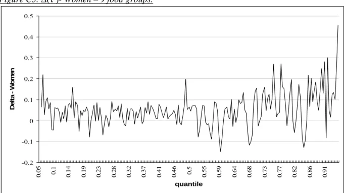
all log prices to their mean+one standard deviation, and other variables to their median (as in Machado and Mata), there are violations for 36:5% and 34:5% of the quantiles for women and men respectively. The results are il-lustrated in Figures C1 and C2 in Appendix C, which represents the value of
( ) = maxnQ^t BM It+1jX0 ; t <
o ^
Q BM It+1jX0 for women and men
respectively, as a function of 2 [0; 1]: when ( ) is negative, there is a
vio-lation. These violations are frequent but generally small: less than 0:131 and 0:080 points of BMI for women and men respectively, in 90% of the cases. Their magnitude is more important in the extreme quantiles (above 0.95)
6.3
Aggregating product categories for greater robustness
Although the above robustness checks rarely appear in empirical papers, they are useful because they indicate the reliability of the empirical inference. Here, they somewhat weaken the main …ndings. However, this may re‡ect the large number of covariates in the model. To illustrate, I now present complementary results obtained by aggregating food categories into nine broad food groups: water, beverages other than water, fruit and vegetables, meat and seafood, dairy products, fats, sugar and confectionery, snacks and ready-meals. For each group k, a price index is constructed as follows:
Pkc= Lk X lk=1 wc lk P lkw c lk pclk
where lk is an index for the Lk food categories making up the functional group
k (e.g. for dairy products: cheese, yoghurt and milk); pc
lk = \ln( c
lk) is the
cluster-speci…c index computed in Section (2); and wclk is the cluster-average
2 1As > 0 and > 0, it can be shown that signh@
X( eEt)=@ eEt i = sign [ X] (with X = l; I) and signh@ 0( eEt)=@ eEt i = signh ( KW+ W W ) KK i where ( KW+ W W ) KK is a
share of household expenditures on lk. The stationary price-BMI equation was
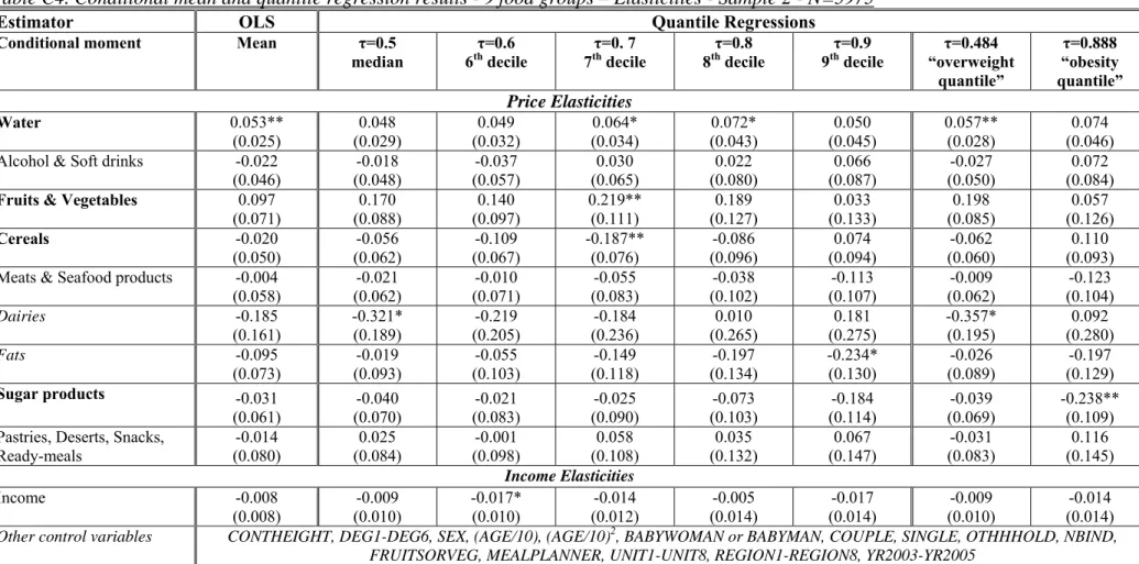
re-estimated via quantile regressions Tables C3 and C4 in Appendix C shows the results for women and men respectively.
Prices are less signi…cant than in Tables C1 and C2. One reason is that some groups (e.g. alcohol and soft drinks) aggregate food categories for which price elasticities had opposite signs in the previous regressions.For women, dairies and fats attract negative coe¢ cients, and the price elasticity of water is positive. For the last category - pastries, deserts , sancks and ready-meals - the positive e¤ect that was found for snacks is clearly dominated by the negative price e¤ects for pastries, deserts and ready-meals. This is not surprising as expenditures on ready-meals, pastries and deserts are higher than expenditures on snacks and, as a consequence, the price of the food group gives less importance to the latter. For man, the elasticities for water and fruits and vegetables are positive and sometimes signi…cant. It is interesting to note that fats and sugar products attract negative coe¢ cients, which are signi…cant only for the highest quantiles. last, negative elasticities are associated to dairies and cereals around the median. These results thus con…rm and strengthen the …ndings in Section 6.
Since there are fewer variables, statistical inference is also more robust, .
The rate of violations (at the design point X0) falls to 23% and 18:5%, for men
and women respectively. Figures C3 and C4 shows that violations are rather small. However, they occur more frequently in the quantiles of the conditional distribution above the median. This calls for caution in the use of the results.
7
Food price policies and the distribution of BMI
A number of elasticities were found to be signi…cant in the regression. These seem to be of small size, which is in line with previous empirical …ndings. Chouet al. (2004) …nd that the elasticity of BMI to food-at-home price is 0:039.
In Powell et al. (2008), the OLS price elasticity of fruit and vegetables is small and insigni…cant (0:012). In quantile regressions, values are between 0:001 at
the median and 0:015 at the 90th quantile. A larger and signi…cant elasticity
is found at the 95th quantile (+0:049), with a potential "extremal quantile" bias (see Chernozhukov, 2005). To our knowledge, only Asfaw (2006) has found strong empirical evidence of price e¤ects, but for a developing country Egypt -with perhaps greater spatial price variation: the BMI elasticities of energy-dense
products (bread, sugar, oil and rice) range between 0:1 .and 0:2, while the
BMI elasticity of fruits was signi…cantly positive (+0:09), as was that on milk and eggs (+0:141).
I will now show that small price elasticities may produce large price e¤ects on the BMI distribution, when the prices of several product categories vary
simultaneously.
7.1
Simulation method
Table C5 translates naively the estimated elasticities in weight changes for a 1:70 meter tall woman, and 1:80 meter tall man. For instance, a 10% decrease in the price of fruit and vegetables in brine would reduce a man’s weight by 1:2 kg, if his initial weight was about 81 kg (at the overweight quantile), and by 1:5 kg if his initial weight was 97:2 kg (at the obesity quantile). A policy that would increase the prices of soft drinks, pastries and deserts, snacks and ready-meals by 10%, and would reduce the price of fruit and vegetables in brine by 10% produces weight losses of 2:6 kg at the overweight quantile and 3:6 kg
at the obesity quantile for men. These numbers are respectively 3:2 kg and
2:9 kg for women.
However, these simulations are naive, because price elasticities at conditional quantiles are not price e¤ects on unconditional quantiles. Moreover, they do not fully pro…t from the advantage of quantile regression over OLS, as the former also provide information on how the unconditional distribution of BMI is a¤ected by price changes, which is more interesting for the simulation of price policies. The method proposed by Machado and Mata (2005) is applied to simulate the marginal densities implied by the conditional quantile model under a given price regime. The procedure consists of …ve steps:
1. Draw a random sample of B numbers from a uniform distribution on [0; 1]:
1, 2; ::; B. Each number represents a quantile of the distribution. Here,
B = 1500.
2. For each quantile b, estimate using the actual data the quantile regression
model (14). This generates B quantile regression parameters b( b), that
can be used to simulate the predicted conditional distribution
3. Generate a random sample of size B by drawing with replacement obser-vations in the actual data set (i.e. from the rows of X): this generates a
sample of size B with typical observation Xi:
4. Then fBMIi = b( b)0Xig is a random sample of the BMI distribution
integrated over the covariates X, i.e. the unconditional distribution of BMI that is consistent with the conditional quantile regressions results. 5. Construct a hypothetical data set from the actual data set, by replacing
actual prices by their desired levels (for instance increase by 1% the price of vegetables). And repeat step 3 to obtain a new sample of size B, and step
4 to obtain the marginal distribution that would prevail under the new price regime. Comparing the latter to the actual (predicted) distribution draws a precise picture of the e¤ect of price policies on the prevalence of
overweight and obesity.22
Con…dence intervals can in theory be constructed by repeating these …ve steps. However, given that the procedure is time-consuming, we here focus on point estimates of the e¤ect of hypothetical policy reforms.
7.2
Results
I now compare the simulated distribution of BMI in the current price regime, and the distribution that would prevail under …ve di¤erent price scenarios. In scenario 1, the price of soft drinks and snacks increases by 10%,while the price of fruits and vegetables in brine decrease by 10%, as suggested by a recent o¢ cial report (IGF-IGAS, 2008). Scenario 2 adds a 10% increase in the price of soft drinks, breaded proteins, pastries and deserts, and ready-meals, but do not decrease the price of fruits and vegetables. In scenario 3, the latter fall again by 10%. Scenario 4 imagines that the prices of fats and sugar and confectionery also increase by 10%. In scenario 5, dairies, especially cheese, which is at the heart of the French gastronomy, also enter in the tax base.
Table C6 reports for each scenario the prevalence of overweight and obesity in the simulated sample before and after the implementation of the policy. Emery et al. (2000) estimate that the extra medical costs associated with obesity vary between 506 Euros and 648 Euros. The lower bound considers only a limited set of medical conditions and individuals with BMI over 30, while the upper bound extends the set of medical conditions and takes into account all individuals with BMI over 27. Hence, by extrapolating the percentages to the entire adult population (about 48:5 million adults in 2004), we have a point estimate of the expected reduction in health-care expenditure. This evaluation does not take into consideration the statistical uncertainty in the estimated conditional quantiles.
The minimum reduction in health care expenditure varies between 534 million Euros (Scenario 1 lower bound) and 2498 milmillion Euros (Scenario 5 -upper bound). Given the regression results, it is not surprising that the larger the tax base, the higher the expected e¤ects. Scenario 3 seems to have a good design, since the tax base does not include symbolic products such as cheese or olive oil, and has sizeable e¤ects. The prevalence of adult obesity would fall by 33%. Figures C5 and C6 in Appendix C present the results for men and