HAL Id: hal-01142357
https://hal.archives-ouvertes.fr/hal-01142357
Preprint submitted on 15 Apr 2015
HAL is a multi-disciplinary open access
archive for the deposit and dissemination of
sci-entific research documents, whether they are
pub-lished or not. The documents may come from
teaching and research institutions in France or
abroad, or from public or private research centers.
L’archive ouverte pluridisciplinaire HAL, est
destinée au dépôt et à la diffusion de documents
scientifiques de niveau recherche, publiés ou non,
émanant des établissements d’enseignement et de
recherche français ou étrangers, des laboratoires
publics ou privés.
cereals supply chain in France
Jean-Yves Courtonne, Julien Alapetite, Pierre-Yves Longaretti, Denis Dupré,
Emmanuel Prados
To cite this version:
Jean-Yves Courtonne, Julien Alapetite, Pierre-Yves Longaretti, Denis Dupré, Emmanuel Prados.
Downscaling material flow analysis: the case of the cereals supply chain in France. 2015.
�hal-01142357�
Jean-Yves Courtonnea,b,d,⇤, Julien Alapetitea, Pierre-Yves Longarettia,c, Denis Dupr´ea,b,
Emmanuel Pradosa
aSTEEP team, INRIA Grenoble - Rhˆone-Alpes, Montbonnot, France
bCentre de Recherches Appliqu´ees `a la Gestion, Universit´e Pierre-Mend`es France, Grenoble, France cUJF-Grenoble 1 / CNRS-INSU, Institut de Plan´etologie et d’Astrophysique de Grenoble (IPAG) UMR 5274
dArtelia Eau et Environnement, Echirolles, France
Abstract
The spatial reconstruction of the production, trade, transformation and consumption flows of a spe-cific material, can become an important decision-help tool for improving resource management and for studying environmental pressures from the producer’s to the consumer’s viewpoint. One of the obstacles preventing its actual use in the decision-making process is that building such studies at var-ious geographical scales proves to be costly both in time and manpower. In this article, we propose a semi-automatic methodology to overcome this issue: we describe our multi-scalar model and its data-reconciliation component and apply it to cereals flows. Namely, using official databases (Insee, Agreste, FranceAgriMer, SitraM) as well as corporate sources, we reconstructed the supply chain flows of the 22 French regions as well as the flows of four nested territories: France, the Rhˆone-Alpes r´egion, the Is`ere d´epartement and the territory of the SCOT of Grenoble. We display the results using Sankey diagrams and discuss the intervals of confidence of the model’s outputs. We conclude on the perspec-tives of coupling this model with economic, social and environmental aspects that would provide key information to decision-makers.
Keywords: material flow analysis, supply chain, downscaling, data reconciliation, cereals, France
⇤Corresponding author
Email addresses: jean-yves.courtonne@inria.fr (Jean-Yves Courtonne), julien.alapetite@gmail.com (Julien Alapetite), pierre-yves.longaretti@inria.fr (Pierre-Yves Longaretti), denis.dupre@iae-grenoble.fr (Denis Dupr´e), emmanuel.prados@inria.fr (Emmanuel Prados)
1. Introduction 1
Material flow analysis (MFA) is a systematic assessment of the flows and stocks of materials within 2
a system defined in space and time (Brunner and Rechberger, 2003). Depending on the pursued ob-3
jective (e.g. detoxification, dematerialization etc.), this framework has been implemented for vari-4
ous scopes de facto creating a family of methodologies, ranging from Substance Flow Analysis to 5
Economy-Wide Material Flow Accounting (Bringezu and Moriguchi, 2002). In this paper, we are in-6
terested in mapping the flow of specific resources throughout the economy, both from a spatial and a 7
processing point of views; i.e., we aim to trace the associated flows from the extraction of raw materials 8
to the processing, trade and consumption of the derived products based on the resource under consid-9
eration. These studies are known as MFA on the level of goods, as defined by Baccini and Brunner 10
(2012)1. In their original work, Billen et al. (1983) conducted such MFA on 6 supply chains at the
11
scale of Belgium (iron, glass, plastic, lead, wood and paper, and food products). Since then, MFA has 12
been mostly applied to metals2 (Ciacci et al., 2013), (Eckelman and Daigo, 2008), (Liu and M¨uller,
13
2013), (Dahlstr¨om and Ekins, 2006), (Bonnin et al., 2012) to cite only a few. Some studies were 14
also undertaken on construction materials (Smith et al., 2003) and wood (Hashimoto and Moriguchi, 15
2004), (Binder et al., 2004), (Cheng et al., 2010). Regarding food products, few studies actually quanti-16
fied flows between the production, transformation and consumption stages (Blezat-Consulting, 2010), 17
rather focusing on the supply of a product unit (Narayanaswamy et al., 2003), (Mintcheva, 2005), 18
(Virtanen et al., 2011), or on regional nitrogen flows (Billen et al., 2009). 19
Binder et al. (2009) raised the important issue of the practical usefulness of large-scale MFA stud-20
ies for policy-making. Three main obstacles were identified in comparison with MFA at the scale of an 21
industrial unit: “(i) the numbers of stakeholders involved increases [...] and it becomes unclear who is 22
responsible for taking action; (ii) the uncertainty of the data increases; and (iii) the goals [...] are not 23
always clearly defined”. In order to bridge the gap between research findings and policy-making, many 24
authors have rightly argued that MFA should be coupled with social, economic or/and environmental 25
models (Binder, 2007). This kind of coupling was for instance successfully implemented by Rochat 26
1Two kind of materials are distinguished: substances, that is any chemical element or compound composed of uniform units,
and goods, that is economic entities of matter with a positive or negative economic value [...] made up of one or several substances (Brunner and Rechberger, 2003).
et al. (2013) who combined MFA, Life Cycle Assessment (LCA) and multi-scenarios, multi-criteria, 27
multi-stakeholders analysis to address the issue of PET plastic management in Columbia. One could 28
also refer to the study carried out by Bouman et al. (2000) who used SFA, LCA and partial equilibrium 29
models to evaluate industrial systems and compare pollution management scenarios. Coupling MFA 30
with a social model aims at better understanding the behaviors of stakeholders and the interactions 31
between them in order to study how to improve resource management. For instance, Binder et al. 32
(2004) used a multi-agent model to study the management of regional wood flows in Switzerland. As 33
mentioned by Kytzia et al. (2004), the coupling of MFA with an economic model can be performed 34
to study economic consequences of environmental policy, or on the contrary, to study the e↵ective-35
ness of economic tools to tackle environmental issues. Finally, the coupling with an environmental 36
model, for example with LCA, makes it possible to build environmental accounts (such as footprints) 37
from the producer’s and from the consumer’s perspective. As underlined by many authors (e.g., Peters 38
and Hertwich 2006; Skelton et al. 2011), these points of view are both complementary and paramount 39
for policy-making. The producer’s point of view informs on environmental pressures that occur on a 40
territory: a variety of measures (incentives, regulations, information...) can be taken to address these 41
pressures. The consumer’s point of view informs on the responsibility of the consumer for environ-42
mental burdens occurring locally or far away (end products purchased by final consumers trigger global 43
supply chains and thus it can be argued that consumers bear the subsequent environmental pressures). 44
The present paper is the first step of a project aiming at analyzing local supply chains from an 45
economic, social and environmental perspective for decision-aiding. In particular we aim at analyzing 46
environmental pressures along supply chains, i.e. from the producer’s to the consumer’s viewpoint. The 47
paper has two main objectives. The first one is to assess the feasibility of downscaling a national MFA 48
to simultaneously obtain MFAs on every subterritory the country is composed of (e.g. every regions). 49
This makes the study more time-efficient while also ensuring the comparability of the data and the 50
consistency of aggregated results (the regional data will sum up to the national data). These results 51
can then serve as a basis for discussion and refinements with local stakeholders. The second goal is 52
to undertake a multi-scale MFA. We strongly believe that multi-scale analysis is a powerful decision-53
help tool given social-environmental issues are unlikely to be resolved at any single administrative 54
level. Such a perspective has already been adopted in France in the case of Paris and its region where 55
economy-wide MFAs were produced on three di↵erent geographical scales (from the city to the r´egion 56
level; Barles (2009)). Here, we undertake studies at the national, regional, departemental and SCOT3
57
scales. 58
In order to illustrate the interest of the tool we have developed, we have chosen to apply it to a basic 59
class of commodities, i.e., cereals. This choice is motivated by the following considerations: 60
• At the world’s scale, but more generally at any scale, the supply of cereals and cereals products 61
is strategic given their direct and indirect (through meat consumption) role in human diets and 62
their increasing use for other purposes (e.g. bioethanol), 63
• Cereals are, in terms of weight of production, the most important agricultural good in France; 64
the supply chain is represented all over the territory and, at the same time, a strong heterogeneity 65
can be observed between regions, 66
• The supply chain is well structured making it easier to model and collect the necessary data. 67
• Finally, it is possible to account for most end-products derived from cereals with a limited set of 68
descriptive product categories, bread being the most obvious one in the case of France. 69
The paper is organized as followed: the first section depicts the methodological framework and the 70
sources and hypotheses used in the modelisation phase, we present and discuss the results in the second 71
section before concluding on the perspectives for further research in the field of MFA. 72
2. Materials and methods 73
2.1. Methodological framework 74
In order to semi-automatically produce MFAs at subnational scales, we start by building a consis-75
tent MFA at the country level. For this purpose, we use on the one hand a supply and use tables (SUTs) 76
framework as a way to present and organize the data, and on the other hand a constraint optimiza-77
tion algorithm aiming at reconciling inconsistent data. We underline here that while we use a typical 78
Input-Output framework, we don’t go into any IOA (e.g. computation of the Leontief matrix)4.
79
It is worth noting our resource-specific MFA based on SUTs is close to the concept of Material 80
System Analysis (MSA) introduced by Moll et al. (2005) on the case of European iron and steel flows, 81
3Sch´ema de coh´erence territoriale: the SCOT is an urban-planning document dedicated to a group of towns or urban areas. 4French IO tables indeed come into a too aggregated form to reach the level of detail we are interested in here.
and taken up by OECD (2008). However, while MSA is considering all material inputs and outputs 82
along the supply chain (i.e. life-cycle-wide), we only focus at this step on one good: cereals5.
83
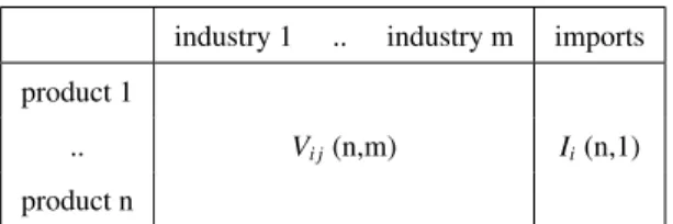
2.1.1. Supply and use tables 84
Handling a large quantity of data is a major difficulty in MFA and calls for a proper way of orga-85
nizing the information. SUTs appear to be the most convenient framework to achieve this goal. They 86
comprise a Supply table, which indicates the origin of the goods (either sector-wise or geographically) 87
and a Use table, which indicates the destination of the goods. 88
5The study of specific material/environmental flows associated with it will be tackled in a next step as described in the
industry 1 .. industry m imports product 1
Vi j(n,m) Ii(n,1)
.. product n
industry 1 .. industry m exports consumption product 1
Ui j(n,m) Ei(n,1) Ci(n,1)
.. product n
As shown above, the supply table comprises the supply matrix V and the imports vector I whereas 89
the use table comprises the use matrix U, the exports vector E and the (final) consumption vector C. 90
For instance Ui j refers to the quantity of product i that is used by sector j and Cirefers to the quantity
91
of product i that is consumed by end-users on the territory. The constraints linking these elements are 92
discussed in section 2.1.3. 93
Using SUTs implies to make a list of the goods deriving from the primary resource under study, 94
i.e. the primary material itself, semi-products, by-products and end-products. Finding the appropriate 95
level of details for both products and industries is an iterative process between looking for sources 96
of information and trying to fill the tables. With a small number of highly aggregated product cate-97
gories, the study isn’t likely to provide useful information and with a very detailed list of products and 98
industries, filling the data, especially at local scales, won’t be feasible. A good knowledge of exist-99
ing classifications in the national statistical system, for instance economic sectors, products or traded 100
commodities classifications, is also required because correspondences between them will be needed. 101
We used the most precise level of classification of economic sectors available in France for most of 102
the sectors in the study: the NAF 2008 classification (732 sub-classes). For some important products 103
such as bioethanol, this classification was however not precise enough. In those cases, we created our 104
own sectors, knowing information on factories location was available from the cereals’ supply chain 105
federation. This initial step of supply-chain structure analysis is the most time-consuming and cannot 106
be automatized. In fact, it consists in building a model of the supply chain: a too coarse model will 107
not make sense while a too detailed one will be intractable. The final version of our study includes 19 108
products and 18 sectors (displayed in figure 11 in Supplementary Material section A). 109
2.1.2. Boundaries of the study, units and allocation choices 110
We used a typology proposed by Nakamura and Kondo (2009) to define the scope of the study. 111
Inputs from sector a to sector b can take three di↵erent forms: primary material inputs, that will 112
be physically incorporated in the production of sector b (e.g. wheat for flour production), material 113
ancillary inputs, that are necessary for production of sector b but not part of it (e.g. machines), and 114
finally flows of services. For this MFA on cereals we track the flows from product to product until 115
cereal grains are no more physically present in the output of the process. Thus, we go for instance from 116
wheat to flour and to bread and biscuits while we stop the study at animal feed without analyzing the 117
embodied cereals in the meat finally consumed (which would be virtual allocation and not a physical 118
flow of cereals). 119
Like other MFA studies on the level of goods, we converted all flows to a common unit6. Here,
120
flows are expressed in cereals grains equivalent (c.g.e.). The c.g.e. weight equals the real weight when 121
the product under consideration is entirely made out of cereals (e.g. flour), otherwise (e.g. bread, 122
beer...), it represents the weight of the cereal content of the product. 123
To sum things up, our SUTs framework distinguishes itself from SUTs traditionally used in national 124
accounts by the finer-grained description of the products and industries categories, by the fact that it 125
focuses on a single supply chain and by the choice of the unit. 126
2.1.3. Data reconciliation 127
The principle of mass conservation provides a few constraints on the SUTs. When the data comes 128
from distinct sources, these constraints are of course very unlikely to be fulfilled. Making the original 129
data fit the constraints is commonly referred to as the data reconciliation process. The constraints are 130
discussed below. 131
We first apply the law of mass conservation on each product: the amount of product that was used 132
during the considered time period by transforming industries, exports and final consumption, had to be 133
supplied by local industries or by imports (constraint 1). The corresponding equation is: 134 X j ˆVi j+ ˆIi= X j ˆ Ui j+ ˆEi+ ˆCi i = 1..n (1) 135
We use hats above letters to refer to the data resulting from the reconciliation process (original 136
data are represented without a hat). In the general case, equation 1 should contain additional terms to 137
account for initial and final stocks (or alternatively one term of stock variation). We however go around 138
this issue as explained in section 2.2.4. Moreover, losses are treated as a sector (without outputs) in 139
matrices U and V . 140
We apply a similar principle of conservation to every transforming industrial sector (constraint 2): 141
the sum of a sector’s inputs is equal to the sum of its outputs: 142 X i ˆVi j=X i ˆ
Ui j j = 1..m and j is a transforming sector (2)
143
6For instance, Binder et al. (2004) and Cheng et al. (2010) convert all flows of wood-related products into their equivalent in
A sector producing raw materials is not concerned by this constraint because it only has outputs. We 144
moreover implement a few process constraints to verify classical technical conversion factors between 145
products (constraint 3). These equations link one or more inputs of a transforming sector with one or 146
more of its outputs. For instance the yield of conversion of wheat grains into flour translates into the 147
following constraint for the milling sector : Sf lour,mills=0.77 ⇤ Uwheat,mills. We present those equations
148
in table 8 in section A of Supplementary Material. Finally, we want all terms to remain positive (con-149
straint 4) and most of the terms to remain null (constraint 5) because of the supply chain modelisation 150
choices (for instance the primary production sector cannot produce transformed products). 151
Our goal is to minimize the discrepancy between original data and estimated/final data while re-152
specting the constraints. This problem can be expressed in many ways depending on the expression 153
of the distance between original and final data. We choose here one of the simplest, a weighted least 154
square problem under constraints: 155 min ✓ X i X j ( ˆVi j Vi j)2 2 Vi j +X i X j ( ˆUi j Ui j)2 2 Ui j +X i ( ˆIi Ii)2 2 Ii +X i ( ˆEi Ei)2 2 Ei +X i ( ˆCi Ci)2 2 Ci ◆
subject to the set of constraints 1 to 5 (3)
In equation 3, refers to the assumed standard deviation of the data. They make it possible to treat 156
data sources di↵erently depending on the assumed (or possibly measured, or constrained) uncertainties 157
on the data. The chosen weights are discussed later in the paper. 158
2.1.4. Downscaling technique 159
From an administrative point of view, metropolitan France is currently divided in 22 administrative 160
r´egions. Each r´egion is further subdivided into d´epartements (96 in total), the next and last admin-161
istrative authority being towns and cities (about 36000 in total). The lack of data at local scale is 162
problematic. The smaller the scale, the less the availability of the data. For this reason, one can try to 163
estimate the missing data using other existing variables along with data available at a larger scale, by 164
defining appropriate proxies. 165
The general proxy expression of the estimation of local data would be: 166
Yn+1= f (Yn,Xn+1
1 , .. ,Xn+1k ) (4)
Here the exponents refer to the geographical level of the data (for instance, if n represents the country 168
level, n + 1 represents the regional level). f is the model linking the quantity of interest at level n, Yn
169
(known), and k explanatory variables available at level n + 1, Xn+1
j , to the quantity of interest at level
170
n + 1 that we are looking for: Yn+1.
171
The possibilities of testing complex proxy models are of course very limited by the scarcity of 172
the information. Researchers who faced the lack of data in their local MFA studies actually used a 173
single proxy (or explanatory variable) to estimate missing data (Barles, 2009) (Kovanda et al., 2009) 174
(Niza et al., 2009). This is usually based on reasonable hypotheses such as “consumption is almost 175
proportional to the population”. We applied the same approach here and conducted linear regression 176
tests whenever the sample existed and was of sufficient size7. We studied the possibility of having a
177
multiple explanatory variables model but concluded it wasn’t robust enough given the limited size of 178
the geographic sample (Smaranda, 2013). Moreover, we found that the R2 index, which represents
179
the proportion of the variability of the sample that has been explained by the model, was high enough 180
in the case of a simple one-explanatory-variable-linear model to consider it satisfactory. Results are 181
presented in Table 4. For instance, if we want to estimate the regional use of wheat by the milling 182
industry in region i, Uri
wheat,mills, with the number of employees working in this sector Emills, equation 4
183
becomes: 184
Uri
wheat,mills = Uwheat,millsf r ⇤ Ermillsi /Emillsf r (5)
185
Once enough direct data or proxies have been gathered, it is possible to fill the SUTs. New columns 186
are added to consider inter-regional trade of good. By construction, the imports of product i to region 187
a from region b, Ira,bi , are equal to the exports of product i from region b to region a, Erb,ai , so we only 188
use the Ir variable (matrix) in the program. We then apply the same data reconciliation process as the 189
one described above. An additional constraint however needs to be implemented: one wants to ensure 190
the coherence of the results regarding aggregation and disaggregation. The regional data must sum up 191
to the national total. With the same notations as above for the exponents, the general expression of the 192
aggregation constraint (constraint 6) is: 193
X
i
ˆXn+1, i= ˆXn where ˆX represent matrix ˆV, ˆU, ˆI, ˆE or ˆC (6)
194
In equation 6, I and E refer to international imports and exports only: there is no aggregation 195
constraint on inter-regional trade. 196
There exists no trade database at subnational scales that perfectly matches our products classifica-197
tion. Therefore, a few traded categories are more aggregated than our own categories. For instance the 198
wheat category in the transport database includes both our common wheat and durum wheat categories. 199
Table 16 in section B of Supplementary Material shows the full correspondence and section B depicts 200
the changes that had to be made to take this limitation into account. 201
Finally, no trade data is available below the level of the d´epartement. Therefore, at this scale, we 202
only compute production and consumption (intermediate and final) flows, using the usual proxis and 203
then apply the resource equals use constraint on each product to determine the amount of net imports 204
(or net exports). Thus, we no longer use any optimization or data reconciliation process below the scale 205
of the d´epartement. 206
2.2. Data sources and hypotheses 207
Figure 11 in Supplementary Material section A shows the classifications used in this study for 208
product and sector categories together with the chosen modelisation of the supply chain: it indicates 209
for instance that the starch industry uses common wheat and ma¨ıze and supplies starch and residues. 210
In order to fill the SUTs, the information we are looking for fall into di↵erent categories: primary 211
production, intermediate consumption, stocks, trade, livestock consumption and final consumption. As 212
mentioned in the previous section, we use direct data when it exists and proxy data otherwise. Each 213
type of information is discussed below in relationship to table 3 that summarizes the sources and table 214
4 that presents the chosen proxies. The question of data uncertainties is discussed in the last paragraph 215
of the section. 216
Item Sour ce Smallest scale av ailable Production of each type of cereals (common wheat, durum wheat, ma ¨ıze, barle y...) Statistique Agricole Annuelle (Agreste): http://acces. agriculture.gouv.fr/disar/faces/ d´epartement (better resolution can be purchased as long as does not go ag ainst statistical secret) Production of intermediate products (flour , bread, biscuits, starch, semolina, pasta, malt, beer ...) Bilans d’appro visionnement (Agreste): http://agreste.agriculture.gouv.fr/ enquetes/bilans- d-approvisionnement/ cereales- riz- pomme- de-terre/ , cereals’ inter -profession http://asset.keepeek.com/ permalinks/domain39/2013/06/04/927- B18-Des_ chiffres_et_des_cereales__edition_2012- 2013_-_ page_a_page.pdf country Animal feed (for cattle, poultry and pigs) Bilans d’appro visionnement (Agreste) country Inputs used by the animal feed industry (Agreste) most of the r´egions International trade of ra w materials and trans-formed products Bilans d’appro visionnement (Agreste) country SitraM database (based on French customs’ data) d´epartement of origin /destination -country of origin /destination National road freight SitraM database (based on the TRM surv ey) d´epartement of origin /destination -d ´epartement of origin /desti-nation National railroad freight SitraM database (based on reports from SNCF -av ailable until 2006) r´egion of origin /destination -r ´egion of origin /destination National riv er freight SitraM database (based on reports from VNF) d´epartement of origin /destination -d ´epartement of origin /desti-nation Cereals’ consumption patterns Babayou et al. (1996) r´egions Table 3: A vailable sources for data in weight unit (all recent years are av ailable when applicable)
Item Pr oxy and sour ce Sample size R 2 (and p-value) Used for scales... Cereals production Arable land (code 211) -CORINE Land Co ver 96 0.95 (2e-62) < d´epartement Total liv estock feed Li vestock at subnational scales -Statistique Agricole Annuelle (Agreste) for r´egions and d´epartements, Recensement G ´en ´eral Agricole 2000 (Agreste) for to wn see the lifestock feed section < country Flour production Emplo yment (sector 10.61A) 12 0.75 (2e-4) < country Production of semolina Number of factories not tested < country Production of cornmeal Number of factories not tested < country Rice transformation Number of factories not tested < country Production of canned corn Number of factories not tested < country Starch production Emplo yment (sector 10.62Z) 3 0.96 (0.13) < country Industrial bread production Emplo yment (sector 10.71A) not tested < country Production of bread in supermark ets Emplo yment (sector 47.11F) not tested < country Craft bread production Emplo yment (sector 10.71C) not tested < country Biscuits production Emplo yment (sector 10.72Z) not tested < country Pasta production Emplo yment (sector 10.73Z) not tested < country Li vestock compound feed production Emplo yment (sector 10.91Z) 18 0.96 (1e-12) < r´egion Malt production Emplo yment (sector 11.06Z) 3 0.99 (0.06) < country Beer production Emplo yment (sector 11.05Z) not tested < country Bioethanol production Number of factories not tested < country Final consumption Population coupled with consumption pattern -Population census (Insee), Babayou et al. (1996) not tested < country Table 4: Chosen proxies. R 2can be interpreted as the fraction of the sample’ s variability that is explained by the linear model. The p-v alues (in brack ets) represent the probability of obtaining a similar or better R 2value if the null hypothesis is true (i.e. if there is no relationship between the explanatory and response variables). One usually assumes the null hypothesis is false when the p-v alue is belo w 0.05. Here, we can validate the explanatory models for cereals, flour and liv estock feed production whereas the samples are too small to validate the starch and malt production models. Insee’ s CLAP database is used to get the number of emplo yees; number and location of factories come from the yearly report of the Passion C ´er ´eales association (inter -profession). Hypotheses were not tested when no data w as found at the re gional scale.
2.2.1. Primary production 217
Detailed data on cereals production is published in the annual agricultural statitics available down 218
to the level of the d´epartement. We therefore used a land-use proxy (see table 4) to estimate the 219
production of cereals at the scale of a group a cities. 220
2.2.2. Intermediate consumption 221
The annual report of the French inter-profession of cereals (Passion-C´er´eales, 2013) provides in-222
formation on the quantities used and produced by di↵erent industries in the supply chain. Based on 223
this data, we established conversion factors between products (table 8 in Supplementary Material sec-224
tion A), that are used to constrain the problem (see section 2.1.3). When the data couldn’t be found 225
in specific regional reports, which is the general case, we estimated the subnational intermediate con-226
sumptions using the downscaling technique presented in the previous section and the proxies in table 227
4. 228
2.2.3. Livestock feed 229
Regional consumption of cereals for livestock feed are not directly known, mainly because the 230
cereals are distributed in various forms: mostly self-consumption at the farm and consumption of 231
industrial compound products, and marginally grains bought by the farmer. We therefore designed 232
a model to estimate these consumptions. Figure 1 presents the general principle of the model: we 233
estimate the local livestock consumption of cereals based on the data on livestock and slaughter and 234
on the nutritional needs of the animals. Data source for livestock, slaughter and production figures are 235
shown in table 3. We estimated the nutritional needs based on zootechny guidebooks (see table 3) and 236
then scaled them in order to make them consistent with the total cereals animal consumption provided 237
in the national accounts of the ministry of agriculture. Table 10 in Supplementary Material section 238
A shows the modeled distribution of cereals feed among the main categories of animals before and 239
after this adjustment process: the scaling ratio obtained is moderate (1.13), indicating that the model 240
is probably robust. In order to derive this table, we distinguished about 20 di↵erent types of animals 241
and products. Tables 11, 12 and 13 in Supplementary Material section A show the original feed intakes 242
per type of animal or product. Care was taken in order to avoid double-counting: either the lifecycle 243
or the annual approach was used for each product. For instance, we use the lifecycle approach for pigs 244
(meaning we multiply the number of pigs slaughtered during one year by the cereals intake of one pig 245
during its lifespan) and the annual approach for nursing cows (meaning we multiply the livestock at the 246
end of the year by the per capita annual feed intake). Once local cereal feed consumption is estimated, 247
we split it between compound feed and raw feed thanks to information and hypotheses on the animal 248
feed industry (tables 3 and 4).
Figure 1: Principles of the livestock feed model. Input data is shown in grey.
249
2.2.4. Stocks 250
Information about stock is partial, notably because of confidentiality issues. Averaging the figures 251
over several years solves this issue since the variations of stock tend to compensate one year after 252
another. For instance, table 9 in Supplementary Material section A shows that stock variation explains 253
up to 12% of the national apparent consumption in 2003 whereas this number falls to -0.6% over the 254
period average. In this work we therefore study the period 2001-2009. 255
2.2.5. Trade 256
As shown in table 3, for the national MFA, we use the imports and exports data of the ministry of 257
agriculture, providing information with detailed product categories directly in weight of grain equiva-258
lent. For MFAs at subnational scales, we use the SitraM database, maintained by the French ministry 259
of ecology. We underline 3 main difficulties with this data : 260
1. We had to design a correspondence table between the transport statistics classification and our 261
own product classification : table 16 in Supplementary Material section A. 262
2. Assumptions had to be made regarding the national trade by railway since the classification 263
is not as detailed as for the other modes of transport: we assume that cereals represent 75% 264
of the “Agricultural products and living animals” category. This is the proportion found for 265
international export by railroad in 2005. 266
3. Theoretically, there is a compatibility issue between data from the customs (international trade) 267
which provides the first origin and final destination of a product and the national data which 268
provides the last loading or unloading of the merchandise. This issue can lead to double counting 269
for regional imports and/or for exports8. We partially solved the problem by redistributing the
270
international trade by sea using the market shares of French harbors for cereals exports. This 271
means in particular that sea exports of regions without any harbors were entirely reallocated to 272
regions with harbors. We were not able to do the same for road, river or railway transport. Still, 273
this operation is significant since more than half the French exports of cereals are made by sea: 274
on average, between 2001 and 2009, France exported about 14 Mt of cereals by sea, 6 Mt by 275
road, 5 Mt by river, and 1,5 Mt by railroad. Table 14 in Supplementary Material section A shows 276
the impact of this operation on the total international exports of every regions. 277
2.2.6. Final consumption 278
Final consumption of cereal products occurs in two forms: food products (bread, biscuits, pasta...) 279
and industrial products (bioethanol and many products derived from starch). In France, local consump-280
tion patterns are not precisely documented, at least not precisely enough to be used in this study. For 281
most of the products, we considered the per capita consumption to be equal all over France. Regarding 282
bread, we used a study depicting the diversity of food consumption patterns in France in the mid 1990’s 283
that presents statistical information on the gap between regional and average consumption of bread per 284
household (Babayou et al., 1996). This consumption estimation is not built as an apparent consumption 285
(resulting from the di↵erence between production, stock variation and trade) but on direct households 286
surveys. Table 15 (supplementary material) presents the adopted regional adjustment factors for per 287
8For instance, French wheat loaded in the Centre r´egion, transported by road to the Rouen harbor and then exported by sea
to Algeria will be counted in the customs statistics as from the Centre r´egion to Algeria and in the national transport statistics as from the Centre r´egion to Rouen, leading to a double-counting of exports of the Centre r´egion.
capita bread consumption, reconstructed from this report. For subregional scales, no data was found 288
in the report. Following the conclusions of Babayou et al. (1996), that the urban vs. rural and north 289
vs. south typology was the most suited to explain the variability in the bread consumption patterns 290
(rather than regional cultural di↵erences for instance), we estimated the gap between local and average 291
consumptions based on this typology. Table 5 shows the corresponding adjustment factors. 292
Urban Rural
North -10% +21%
South -7% +25%
Table 5: Per capita bread consumption variability among di↵erent categories of towns in the mid 1990’s in France (Babayou et al., 1996). The table makes the distinction between cites in the north and in the south of France and between urban and rural cities (cities with less than 2000 inhabitants are considered rural). According to these authors, this typology is the most suited to explain the di↵erences between bread consumption patterns in France.
According to the national MFA, bread accounts for about 40% of the consumption of cereals for 293
food purposes, and for one third of the total consumption of cereals. This adjustment on local bread 294
consumption is therefore significant. 295
2.2.7. Data uncertainty 296
Uncertainties on input data 297
Laner et al. (2014) review existing literature regarding uncertainty handling in MFA and provide rec-298
ommendations relatively to the goals of each study. Our case study typically falls in the category of 299
descriptive MFA as they describe it and we use an approach similar to the one implemented in software 300
STAN (Cencic and Rechberger, 2008): input data are expressed by a mean and a standard deviation 301
reflecting the level of confidence in the data. As we mentioned in section 2.1.3, the weighted least 302
squares optimization leads to higher alteration (di↵erence between output and input data) of variables 303
with higher uncertainties. Since none of the sources used provides detailed information on data uncer-304
tainty, this step is based on assumptions and on educated guesses. Following Danius (2002), we treat 305
data di↵erently depending on its origin. Below, we list the di↵erent origins from the ones we trust the 306
most to the ones we trust the less: 307
1. official statistics at local, regional or national scale, based on cross-checking of surveys (some of 308
which are exhaustive) : e.g. agricultural production, employment... 309
2. statistics based on declarations (and punctual control): e.g. customs, reporting from the supply 310
chains’ federations... 311
3. modelised local data, based on downscaling, 312
4. extrapolation of statistical surveys on sub-populations 313
The last one typically applies to road freight statistics which are based on a survey9. The estimation of
314
total road freight in the country (all goods combined) is quite accurate (less than 1% of error according 315
to the calculation of the statistical office (SOeS, 2012)), however the extrapolation on subpopulations, 316
meaning on specific goods in specific regions, can be deteriorated a lot because of the small size of 317
the sample. Collaboration with the statistical office is in progress in order to estimate the intervals 318
of confidence on these subpopulations. Generally we consider that small flows have a larger relative 319
error than large ones for data extracted from the same source, but we prevent null flows from having a 320
vanishing standard deviation (this would be unrealistic). 321
Although the attribution of uncertainty weights is based on objective elements such as the source 322
of the data, this part of the process is not the most robust and the model would benefit from a sen-323
sitivity analysis that would show the impact of a change for each input variable. This was however 324
too demanding to accomplish in this paper (this would require to rewrite our Matlab code in a more 325
efficient language such as C for the simulations for the computational time to remain within reasonable 326
bounds). 327
Uncertainties on output data 328
Using common terminology in statistics, we can describe our problem as follow: if we call a supply-329
use table with uncertainties on each parameter a supply-use table distribution (STUD), then our goal 330
is to obtain a posterior STUD from our prior STUD. Given the number of constraints we know our 331
result is of much lower dimension than the number of variables and a direct sampling of the posterior 332
STUD is then possible by Monte-Carlo simulations. The intervals of confidence of output variables are 333
thus inferred from theses simulations. Numerous input datasets are randomly generated knowing the 334
standard deviation of input data, and assuming a Gaussian distribution (although this is not a require-335
ment). After a while, typically in our case, a few tens of simulations, the process reaches convergence. 336
The confidence intervals represented on the diagrams correspond to two standard deviations (95% of 337
possible values if the actual distributions are indeed gaussian). We analyze the results in section 3. 338
2.3. Software integration 339
We wrote a program to properly integrate our databases, the original SUTs, the optimization and 340
Monte-Carlo processes, and the visualization of results. As table 6 illustrates, it made it possible to 341
implement a model with a large quantity of variables, simultaneously computing all sub-entities of a 342
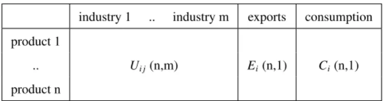
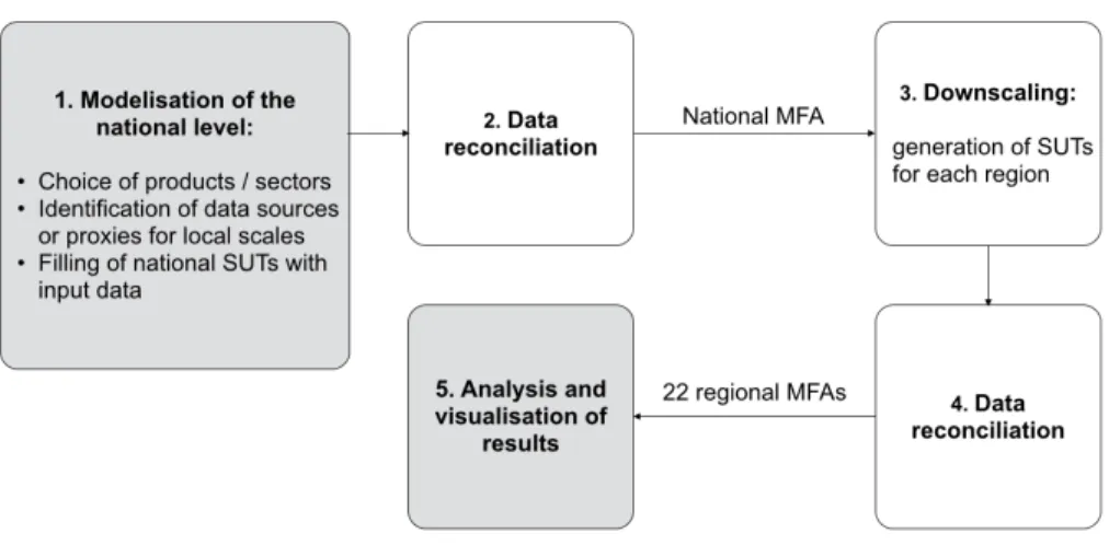
given territory. Figure 2 presents the software background on the study in relation to figure 3 which 343
shows the manual and automatic steps conducted to produce regional results. 344
Geographical scope
Scale Number of MFAs (ter-ritories) computed
Number of output variables (of which are forced equal to zero)
Execution time
France France 1 741 (637) about 10 secs
France Regions 22 25498 (14428) about 40 min
Rhˆone-Alpes Departements 8 13832 (5582) about 10 min
Table 6: Characteristics of each run of the model (one line corresponds to one run). We first obtain the national MFA, then downscale it to obtain results in every region, and finally downscale the Rhˆone-Alpes results in every departement of the region. The 741 variables of the first run are decomposed as follow: 361 variables for the supply table (19 products * 18 sectors + 19 variables for international imports) and 380 variables for the use table (19 products * 18 sectors + 19 variables for international exports + 19 variables for consumption). The 25498 variables of the second (regional) simulation are decomposed as follow: 16302 for the ”basic” supply and use tables (22 regions * 741 variables), 9196 variables for inter-regional trade. We use sparse matrices for the computation as many variables are null (see constraint 5 in section 2.1.3)
Figure 2: The chain of computation and integration between softwares.
3. Results and discussion 345
We use Sankey diagrams to display our results10. They have long been used in flow studies and are
346
very efficient in wrapping a large quantity of information (Schmidt, 2008). We use the following con-347
vention: flows circulating inside the territory are represented by horizontal lines while flows entering 348
or leaving it are represented by vertical lines. Although the core of the paper only shows results under 349
this form, all input and ouput datasets are available by request to the authors. 350
3.1. Results for France and French regions 351
We split the national results into two diagrams in order to make them more readable. Figure 4 shows 352
the production, imports and exports of cereals as well as the flows related to livestock consumption (raw 353
or compound feed). With a yearly average of 34 Mt of grains produced, common wheat is the most 354
commonly grown cereal in France (53% of the total cereal production) before corn (23%) and barley 355
(16%). This production of about 65 Mt is mainly dedicated to exports (about 27 Mt or 42%). Although 356
the information doesn’t appear on the diagram, about 2/3 of these exports go to European countries and 357
1/4 to African and middle-east countries, according to customs data. The rest of the production goes to 358
livestock feed (about 22 Mt or 34% evenly divided between raw and compound feed) and other interior 359
uses (about 16 Mt or 25%). Imports are almost negligible (less than 1 Mt)11. Finally cereals grouped
360
in the other cereals category are only used for exports and for livestock, except for rice. 361
10There is a clear link between SUTs and their representation in Sankey diagrams. Products, and activities (industries, imports,
exports and consumption) are the nodes of the diagram. The values in the supply table are represented by links going from activity nodes to product nodes and the values in the use table are represented by links going from product nodes to activity nodes. For the purpose of this study we developped a Sankey software that can be used on www.eco-data.fr/tools/sankey/start.php
11It can be noted that French livestock depends a lot on imports of soycakes (nearly 5 Mt are imported each year, mostly from
Figure 4: Cereals MFA at the scale of France: international trade and animal feed. Results are shown in kilotonnes for an average year over the period 2001-2009.
Figure 5 shows the interior use of each cereal along with imports and exports of transformed prod-362
ucts, until final human consumption on the territory. Starch and wheat mill industries clearly stand out 363
as the two main supply chains with respectively 6.2 Mt and 4.4 Mt of grain (wheat and corn) processed. 364
They also produce most of the by-products (3.3 Mt or 81% of the residues). Then comes the malting 365
industry with about 1.6 Mt of barley processed. Other supply chains (bioethanol, pasta and couscous, 366
rice, canned corn, cornmeal) are less significant although together, they add up to 2 Mt12. On the
im-367
ports side, the main flows correspond to flour, starch and glucose, pasta and rice, adding up to 1.1 Mt 368
or 85% of the total imports of transformed products. On the exports side, the main flows correspond 369
to starch and glucose, malt and flour adding up to 2.9 Mt or 78% of the total exports of transformed 370
products. On the consumption side, the main flow corresponds to bread (with 2.6 Mt or 34%), starch 371
and glucose (with 1.8 Mt or 23%), and biscuits (with 1.2 Mt or 16%). Pasta, beer, rice, bioethanol, 372
flour, canned corn add up to 2.2 Mt. 83% of cereals are consumed through food and drink products and 373
17% through other industrial products13. All these figures provide convenient points of comparison for
374
sub-national geographic levels. 375
500 Monte-Carlo simulations were conducted for the national model. On average, convergence 376
is observed after 50 simulations: after that the increase of the standard deviation is smaller than 5%. 377
According to the Monte-Carlo process, the range of coefficients of variation goes from 1% to 20%, 378
small flows having a larger relative interval of confidence (i.e. a bigger relative uncertainty) in the 379
general case. The output uncertainty has been reduced compared to the input uncertainty through the 380
enforcement of the constraints, for instance wheat production uncertainty (expressed as the coefficient 381
of variation) goes from 2% in the input to 1% in the output. Finally, we checked that each output value 382
belong to the 95% confidence interval of the input. 383
Figures 12, 13, 14, 15 and 16 in supplementary materials show MFAs of five regions (among the 384
22 computed) each of which present a specific profile (producing region, livestock region, region with 385
a large transformation activity, exporting region...). Considering the whole dataset, figure 6 show the 386
most important flows accross regions. 3 types of flows stand out: most of them are linked to interna-387
tional exports, some other to livestock activities in Bretagne and the rest to transformation activities in 388
12Bioethanol production increased a lot from the end of the 2000-2010 decade: in 2013, about 2.2 Mt of cereals were used for
this purpose, compared to the 0.5 Mt that appear in our results for the 2001-2009 yearly average.
Nord-Pas-de-Calais. These flows result from the model, they are not the mere visualization of the trade 389
database. Firstly, the model output flows distinguish between products that are otherwise grouped in 390
the trade classification: for instance common and durum wheat as well as residues and livestock feed 391
are initially grouped. Secondly, given their high uncertainty compared to other flows (e.g. production), 392
output inter-regional trade flows sometimes di↵er significantly from input values: for instance the orig-393
inal database doesn’t mention any export above 500 kt from the Centre region while the map shows 4 394
flows leaving this region. 395
Figure 6: Flows of cereals > 500 kt/year (average during the 2001-2009 period). The main two countries of destination are shown for each international export flow. AL: Algeria, BE: Belgium, CH: China, EG: Egypt, GE: Germany, IT: Italy, NE: Netherlands, SA: Saudi Arabia, SP: Spain, UK: United Kingdom.
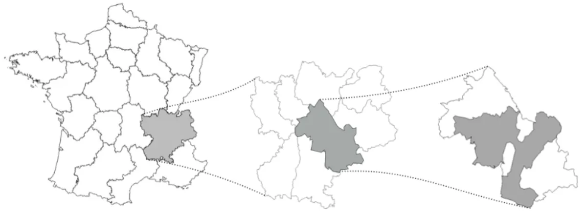
3.2. Multi-scale analysis 396
Figure 7: Nested territories under study. From let to right: France, Rhˆone-Alpes r´egion, Is`ere d´epartment and the territory of the SCOT of Grenoble.
Territory Area (km2) Population (thousands of inhabitants
in 2007) France (metropolitan area) 547030 61796
Rhˆone-Alpes region 44749 6066
Is`ere department 7882 1179
SCOT of Grenoble 3720 714
We show diagrams in an aggregated form in order to make the comparison between geographical 397
scales clearer14. As indicated in section 2.1.4, results at the level of the Scot (that is, below the level
398
of the d´epartement) are not obtained through the usual optimization process and only show net trade. 399
Results for the Is`ere d´epartement are skipped, because they were close to what is observed at the Scot 400
level, but are available upon request. 401
14The graphical scale (i.e. width of line per kt) is di↵erent in diagrams 8, 9 and 10 in order to improve the readability of the
Figure 9: Cereals MFA at the scale of the Rhˆone-Alpes region: aggregated results shown in kilotonnes for an average year over the period 2001-2009.
Figure 10: Cereals MFA on the territory of the SCOT of Grenoble: aggregated results shown in kilotonnes for an average year over the period 2001-2009.
The comparison of figures 8 and 9 shows that the supply chain’s structure at the level of France and Rhˆone-Alpes 402
are very di↵erent15. Indeed, unlike France:
403
• With a yearly average of 1.1 Mt of grains produced, corn is the most commonly grown cereal in Rhˆone-Alpes 404
(51% of the total cereal production) before common wheat (29%), 405
• The region is not caracterized by a significant net export capacity, human and livestock consumption almost 406
adding up to local production, however, inter-regional trade has a important role in the working of the supply 407
chain. In particular, the region is a net exporter of corn, inter-regional exports being the biggest outlet of the 408
corn supply (with 55%), whereas it is a net importer of common wheat (38% of the supply comes from outside 409
the territory), 410
• Many industries, such as the starch industry, are not represented in the region, which leads to significant imports 411
of transformed products (in fact, regional industries almost exclusively process common and durum wheat). 412
100 Monte-Carlo simulations were run at the regional level. On average, convergence is observed after about 413
50 simulations. Each flow from one region to another has been computed by the model. We however only show 414
aggregated results because they come with a smaller uncertainty range. As we can see on figure 9, uncertainty ranges 415
of trade flows (even aggregated) are usually quite large. For instance the 95% confidence interval of imports of 416
cereals indicates that the flow can reasonably take values from 301 kt to 1105 kt, the most likely being 703 kt. Of 417
course this reflects the choices made for the uncertainty of input data, where region-to-region flows were given a high 418
uncertainty for the reasons discussed in section 2.2.7. 419
If we now turn to the comparison of the Rhˆone-Alpes and of the Scot of Grenoble’s supply chains, we can see 420
that they share many characteristics. One of the possible explanation is that the territory of the Scot is a small image 421
of the region itself, since it comprises both mountain and plain areas. Two di↵erences are however worth pointing 422
out: the relative net exports capacity of the Scot is larger than the region’s, and contrarily to what happens in Rhˆone-423
Alpes, in the Scot, human consumption is larger than livestock consumption. Corn is the most commonly grown 424
cereal in the Scot whereas wheat is the only cereal processed for human consumption purposes. This implies that 425
the territory depends on imports for the supply of many transformed products. This is not necessarily problematic 426
in itself (the smaller the area the less likely it is to be self-sufficient), but we point out that the multi-scale analysis 427
provides information, e.g., on the range of scale this situation can be found. 428
3.3. Potential interest for practical policy-making 429
The national MFA as well as the study of interregional flows points to the fact that the cereals supply chain 430
is export-oriented. The fact most exported goods are raw materials can raise the question of lost added value and 431
employment on the national territory. Furthermore, being able to compare regions is important for national objectives. 432
For instance, it makes it possible to assess the pros and cons of regional specialization strategies on the three fronts 433
of sustainability (economic, social and environmental). 434
From another angle, the type of tool described here is potentially helpful for a better integration of the di↵erent 435
levels of decisions through the ability to analyze more and more detailed geographical scales. In the case of France, 436
various administrative levels have leverage on some parts of the supply chain, and each one on a di↵erent aspect. For 437
instance, local (group of cities) levels can foster or discourage the development of certain type of activities, either 438
through subsidies, public orders (e.g. organic food in schools) or by administrative authorizations. The regional 439
level is often in charge of coordinating local initiatives while the global strategy and objectives are established at 440
the national level. A multi-scale tool can help in identifying more efficiently the most appropriate type and level of 441
decisions for a given objective. 442
Generally speaking, through the analysis of the most important supply chains present at the various geographic 443
scales (a substantial endeavor in itself) one opens up the possibility of addressing a number of social and environmen-444
tal issues and of identifying potential lock-ins and/or leverages for a sustainability transition; we briefly mention a few 445
key questions here. What are the critical supply chains in terms of employment for a given territory? What are their 446
weaknesses and opportunities relatively to the territory’s resources (in a wide meaning of the word)? What type of 447
environmental impacts are associated to them, and where do they occur (is the territory externalizing major impacts)? 448
Regarding the case of cereals, energy use / emission of greenhouse gases, use of water and use of pesticides are of 449
particular interest. A production map coupled with ecosystem services analyzes16 will show what are the critical
450
areas/productions, while the supply chain point of view will show how impacts can be shared between producers and 451
consumers. A supply chain perspective may also help decision-makers anticipate climate change impacts (e.g., how 452
a change in cereal production type and pattern a↵ects employment and/or consumption on the territory?) Conversely, 453
how can consumer-driven sustainability demands (local production, for example, or reduction of demand for meat-454
based products) a↵ect existing supply chains and promote new ones, both in terms of employment and (local and 455
distant) environmental impacts? Addressing a number of these questions will of course require a scenario approach, 456
or at least an analysis of contrasted options. 457
4. Conclusion 458
Regarding our first objective, that is assessing the feasability of constructing non-survey MFA at local scales, 459
we argue that the proposed methodology is an efficient investment: e↵orts are needed to design the initial model 460
(in relation to the downscaling objective) but results are then available almost directly for any territory covered by 461
the data. Moreover, the data reconciliation process provides consistent and comparable results among territories. 462
Secondly, we tested our multi-scale model and analyzed its results in the case of the cereals supply chain of four 463
nested territories: France, the Rhˆone-Alpes r´egion, the Is`ere d´epartement and the SCOT of Grenoble. This example 464
shows that it is possible to identify the key di↵erences in local supply chains and to understand how they are currently 465
articulated. 466
Uncertainties are unavoidable in this kind of studies and it is important to assess them (Rechberger et al., 2014). 467
We tried to do so, although acknowledging that the evaluation itself is still imperfect. In order to improve it, at least 468
three elements would be useful: an iteration with local stakeholders and experts during the design of the model and 469
the choice of data inputs, a better knowledge on the interval of confidence of statistical data used as input (work is 470
for instance under way regarding road freight statistics), and finally, a sensitivity analysis to understand the weight of 471
each input variable in the results of the model. 472
As underlined in the introduction, we consider MFA as a first step towards a broader analysis of economic, 473
social and environmental aspects of local supply chains. Additional work has to be conducted to reach this goal. 474
For instance, regarding environmental aspects, studying the coupling between material flows and the associated 475
major environmental footprints (energy use, greenhouse gases emissions, water use, use and emission of pollutants...) 476
provides relevant leads for our future investigations of this topic. MFA helps to bridge the geographical gap between 477
producers and consumers and can provide good insights on their shared responsibility. 478
Calame and Lalucq (2009) argue that subnational territories and supply chains are the two key players for orga-479
nizing a sustainable society in the 21stcentury thus replacing the the couple state - company, which played a pivotal
480
role in the 20thcentury, but which they find ill-suited to face the new challenges of sustainability). In their opinion,
481
they could organize both territorial coherence (from city to regional scale) and production chains. There are several 482
underlying ideas to these statements. Firstly, by insisting on supply chains rather than on the companies, one brings 483
the collaborative aspect of exchanges to the forefront to balance the competitive aspects of free markets. Secondly, 484
the focus on territories is driven by the necessity of building on local strengths to balance local weaknesses in the 485
undertaking of a sustainability transition. Finally, local/regional levels are more reactive, and closer to actual social 486
needs and environmental threats, although of course a multiplicity of approaches targeted at the whole spectrum of 487
decision scales is needed to address sustainability issues. 488
The present MFA study is one of the tools that can be used to foster such a view, as it has the potential to 489
meet decision-makers concerns by providing key information on local supply chains viewed from the economic 490
(creation of wealth), social (local employment) and environmental (flows of environmental pressures from producers 491
to consumers) perspectives. In a time when the fragility of the complex globalized system makes it mandatory 492
for all to strengthen their capacity of absorbing exogenous shocks, the development of such tools at the service of 493
subnational institutions is a necessity. 494
Acknowledgments: This research has been funded by grants from Inria and Artelia Eau & Environnement. 495
496
References 497
Babayou, P., Volatier, J.-L., Chambolle, M., 1996. Les disparit´es r´egionales de la consommation alimentaire des 498
m´enages franc¸ais :. CREDOC, Paris. 499
URL http://bibliotheque.insee.net/opac/index.php?lvl=notice_display&id=118710 500
Baccini, P., Brunner, P. H., Mar. 2012. Metabolism of the Anthroposphere - Analysis, Evaluation, Design 2e, ´Edition : 501
2nd edition Edition. MIT Press, Cambridge, Mass. 502
Barles, S., Dec. 2009. Urban metabolism of paris and its region. Journal of Industrial Ecology 13 (6), 898–913. 503
URL http://onlinelibrary.wiley.com/doi/10.1111/j.1530-9290.2009.00169.x/abstract 504
Billen, G., Barles, S., Garnier, J., Rouillard, J., Benoit, P., Mar. 2009. The food-print of paris: long-term reconstruc-505
tion of the nitrogen flows imported into the city from its rural hinterland. Regional Environmental Change 9 (1), 506
13–24. 507
URL http://link.springer.com/article/10.1007/s10113-008-0051-y 508
Billen, G., Toussaint, F., Peeters, P., Sapir, M., Steenhout, A., Vanderborght, J.-P., 1983. L’´ecosyst`eme Belgique: 509
essai d’´ecologie industrielle. Centre de recherche et d’information socio-politiques. 510
Binder, C. R., Nov. 2007. From material flow analysis to material flow management part i: social sciences modeling 511
approaches coupled to mfa. Journal of Cleaner Production 15 (17), 1596–1604. 512
URL http://www.sciencedirect.com/science/article/pii/S0959652606003106 513
Binder, C. R., Hofer, C., Wiek, A., Scholz, R. W., May 2004. Transition towards improved regional wood flows by 514
integrating material flux analysis and agent analysis: the case of appenzell ausserrhoden, switzerland. Ecological 515
Economics 49 (1), 1–17. 516
URL http://www.sciencedirect.com/science/article/pii/S0921800904000230 517
Binder, C. R., Van Der Voet, E., Rosselot, K. S., Oct. 2009. Implementing the results of material flow analysis. 518
Journal of Industrial Ecology 13 (5), 643–649. 519
URL http://onlinelibrary.wiley.com/doi/10.1111/j.1530-9290.2009.00182.x/abstract 520
Blezat-Consulting, 2010. Etude sur la logistique alimentaire en rhˆone-alpes et ses flux de mati`eres. 521
Bonnin, M., Azzaro-Pantel, C., Pibouleau, L., Domenech, S., Villeneuve, J., 2012. Development of a dynamic mate-522
rial flow analysis model for french copper cycle. In: Computer Aided Chemical Engineering. Vol. 30. Elsevier, pp. 523
122–126. 524
URL http://oatao.univ-toulouse.fr/8375/ 525
Bouman, M., Heijungs, R., van der Voet, E., van den Bergh, J. C. J. M., Huppes, G., Feb. 2000. Material flows and 526
economic models: an analytical comparison of SFA, LCA and partial equilibrium models. Ecological Economics 527
32 (2), 195–216. 528
URL http://www.sciencedirect.com/science/article/pii/S0921800999000919 529
Bringezu, S., Moriguchi, Y., 2002. Material flow analysis. In: Ayres, R., Leslie, A. (Eds.), Handbook of industrial 530
ecology. Edward Elgard Publishing, Cheltenham, pp. 79–90. 531
Brunner, P. H., Rechberger, H., Oct. 2003. Practical Handbook of Material Flow Analysis, 1st Edition. CRC Press, 532
Boca Raton, FL. 533
Calame, P., Lalucq, A., 2009. Essai sur l’oeconomie. Charles L´eopold Mayer. 534
Cencic, O., Rechberger, H., 2008. Material flow analysis with software stan. Journal of Environmental Engineering 535
Management 18 (1), 3–7. 536
Cheng, S., Xu, Z., Su, Y., Zhen, L., May 2010. Spatial and temporal flows of china’s forest resources: Development 537
of a framework for evaluating resource efficiency. Ecological Economics 69 (7), 1405–1415. 538
URL http://www.sciencedirect.com/science/article/pii/S0921800909001335 539
Ciacci, L., Chen, W., Passarini, F., Eckelman, M., Vassura, I., Morselli, L., Mar. 2013. Historical evolution of anthro-540
pogenic aluminum stocks and flows in italy. Resources, Conservation and Recycling 72, 1–8. 541
URL http://www.sciencedirect.com/science/article/pii/S0921344912002182 542
Dahlstr¨om, K., Ekins, P., Jun. 2006. Combining economic and environmental dimensions: Value chain analysis of 543
UK iron and steel flows. Ecological Economics 58 (3), 507–519. 544
URL http://www.sciencedirect.com/science/article/pii/S092180090500337X 545
Danius, L., 2002. Data uncertainties in material flow analysis. KTH, Royal Institute of Technology, Sweden. 546
Drogoul, C., Gadoud, R., Joseph, M.-M., Jussiau, R., Sep. 2004. Nutrition et alimentation des animaux d’´elevage : 547
Tome 2, ´Edition : 2e ´edition Edition. Educagri, Dijon. 548
Eckelman, M. J., Daigo, I., Sep. 2008. Markov chain modeling of the global technological lifetime of copper. Eco-549
logical Economics 67 (2), 265–273. 550
URL http://www.sciencedirect.com/science/article/pii/S0921800908002450 551
Hashimoto, S., Moriguchi, Y., 2004. Data book: material and carbon flow of harvested wood in Japan. Center for 552
Global Environmental Research, National Institute for Environmental Studies, Tsukuba. 553
URL http://www.cger.nies.go.jp/publications/report/d034/D034.pdf 554
Kovanda, J., Weinzettel, J., Hak, T., Mar. 2009. Analysis of regional material flows: The case of the czech republic. 555
Resources, Conservation and Recycling 53 (5), 243–254. 556
URL http://www.sciencedirect.com/science/article/pii/S0921344908002103 557
Kytzia, S., Faist, M., Baccini, P., Oct. 2004. Economically extended-MFA: a material flow approach for a better 558
understanding of food production chain. Journal of Cleaner Production 12 (8-10), 877–889. 559
URL http://www.sciencedirect.com/science/article/pii/S0959652604000691 560
Laner, D., Rechberger, H., Astrup, T., May 2014. Systematic evaluation of uncertainty in material flow analysis. 561
Journal of Industrial Ecology, n/a–n/a. 562
URL http://onlinelibrary.wiley.com/doi/10.1111/jiec.12143/abstract 563
Liu, G., M¨uller, D. B., Oct. 2013. Mapping the global journey of anthropogenic aluminum: A trade-linked multilevel 564
material flow analysis. Environmental Science & Technology 47 (20), 11873–11881. 565
URL http://dx.doi.org/10.1021/es4024404 566
Mintcheva, V., Jun. 2005. Indicators for environmental policy integration in the food supply chain (the case of the 567
tomato ketchup supply chain and the integrated product policy). Journal of Cleaner Production 13 (7), 717–731. 568
URL http://www.sciencedirect.com/science/article/pii/S0959652604000411 569
Moll, S., Acosta, J., Sch¨utz, H., 2005. Iron and steel, a materials system analysis - pilot study examining the material 570
flows related to the production and consumption of steel in the european union. 571
URL http://scp.eionet.europa.eu/wp/wp3_2005 572
Nakamura, S., Kondo, Y., Feb. 2009. Waste Input-Output Analysis: Concepts and Application to Industrial Ecology. 573
Springer Science & Business Media. 574
Narayanaswamy, V., Scott, J. A., Ness, J. N., Lochhead, M., Jun. 2003. Resource flow and product chain analysis as 575
practical tools to promote cleaner production initiatives. Journal of Cleaner Production 11 (4), 375–387. 576
URL http://www.sciencedirect.com/science/article/pii/S0959652602000598 577
Niza, S., Rosado, L., Ferr˜ao, P., Jun. 2009. Urban metabolism. Journal of Industrial Ecology 13 (3), 384–405. 578
URL http://onlinelibrary.wiley.com/doi/10.1111/j.1530-9290.2009.00130.x/abstract 579