HAL Id: hal-00295575
https://hal.archives-ouvertes.fr/hal-00295575
Submitted on 10 Jan 2005
HAL is a multi-disciplinary open access
archive for the deposit and dissemination of
sci-entific research documents, whether they are
pub-lished or not. The documents may come from
teaching and research institutions in France or
abroad, or from public or private research centers.
L’archive ouverte pluridisciplinaire HAL, est
destinée au dépôt et à la diffusion de documents
scientifiques de niveau recherche, publiés ou non,
émanant des établissements d’enseignement et de
recherche français ou étrangers, des laboratoires
publics ou privés.
Stratospheric age of air computed with trajectories
based on various 3D-Var and 4D-Var data sets
M. P. Scheele, P. C. Siegmund, P. F. J. Velthoven
To cite this version:
M. P. Scheele, P. C. Siegmund, P. F. J. Velthoven. Stratospheric age of air computed with trajectories
based on various 3D-Var and 4D-Var data sets. Atmospheric Chemistry and Physics, European
Geosciences Union, 2005, 5 (1), pp.1-7. �hal-00295575�
www.atmos-chem-phys.org/acp/5/1/ SRef-ID: 1680-7324/acp/2005-5-1 European Geosciences Union
Chemistry
and Physics
Stratospheric age of air computed with trajectories based on various
3D-Var and 4D-Var data sets
M. P. Scheele, P. C. Siegmund, and P. F. J. van Velthoven
Royal Netherlands Meteorological Institute (KNMI), P.O. Box 201, 3730AE, De Bilt, The Netherlands Received: 11 June 2004 – Published in Atmos. Chem. Phys. Discuss.: 20 August 2004
Revised: 1 November 2004 – Accepted: 15 December 2004 – Published: 10 January 2005
Abstract. The age of stratospheric air is computed with a
trajectory model, using ECMWF ERA-40 3D-Var and op-erational 4D-Var winds. Analysis as well as forecast data are used. In the latter case successive forecast segments are put together to get a time series of the wind fields. This is done for different forecast segment lengths. The sensitivity of the computed age to the forecast segment length and as-similation method are studied, and the results are compared with observations and with results from a chemistry transport model that uses the same data sets. A large number of back-ward trajectories are started in the stratosphere, and from the fraction of these trajectories that has passed the tropopause the age of air is computed. First, for ten different data sets 50-day backward trajectories starting in the tropical lower stratosphere are computed. The results show that in this re-gion the computed cross-tropopause transport decreases with increasing forecast segment length. Next, for three selected data sets (3D-Var 24-h and 4D-Var 72-h forecast segments, and 4D-Var analyses) 5-year backward trajectories are com-puted that start all over the globe at an altitude of 20 km. For all data sets the computed ages of air in the extratropics are smaller than the observation-based age. For 4D-Var forecast series they are closest to the observation-based values, but still 0.5–1.5 year too small. Compared to the difference in age between the results for the different data sets, the differ-ence in age between the trajectory and the chemistry trans-port model results is small.
1 Introduction
The mean age of air (Hall and Plumb, 1994) is a diagnostic applied to evaluate the transport of tracers by the Brewer-Dobson circulation in atmospheric chemistry transport
mod-Correspondence to: M. P. Scheele
(scheele@knmi.nl)
els (CTMs). It can be defined as the time that air has resided in the stratosphere after entering it through the tropopause.
In a recent study by Meijer et al. (2004), the stratospheric age of air in a CTM (the TM4 model), driven by differ-ent data sets from the European Cdiffer-entre for Medium-Range Weather Forecast (ECMWF), was compared to the age of air, calculated from observations (Andrews et al., 2001). The re-sults showed that in the extratropics at 20 km altitude the simulated age of air was about half that of the observation-based age. The precise reason for this is not clear. It could be due to the preprocessing, involving interpolations, that the ECMWF data undergo before they can be used to drive the TM4 model (Bregman et al., 2003), but also to errors in the original ECMWF horizontal and vertical stratospheric wind data themselves (van Noije et al., 2004).
Errors in the original circulation data can be due to the as-similation of new observations, which slightly disturbs the physical balance. Weaver et al. (1993) found that data assim-ilation leads to overestimation of vertical transport. Noise, introduced in the model by assimilation can be avoided by using data from a general circulation model (GCM). Tan et al. (2004) showed that mixing in analyzed winds is signifi-cantly larger than mixing in GCM winds. Using a trajectory model, Schoeberl (2003) showed that the age of stratospheric air computed from analyzed winds is smaller, and less real-istic, than the age computed from GCM winds.
If real-atmospheric data are to be used, a GCM cannot be applied and assimilation errors seem unavoidable. However, the magnitude of these errors depends on the type of data that is used. Bregman et al. (2003) found that vertical transport in a CTM was more realistic when computed from 4D-Var than from 3D-Var analyses. In an ozone transport study with a CTM, Wild et al. (2003) used sequences of forecast series instead of analyses. The use of forecast data was motivated by the large dynamical self-consistency of these data relative to that of analyses.
2 M. P. Scheele et al.: Trajectories-based age of air In the present study we use a trajectory model to compute
the age of air, using different types of ECMWF wind analy-ses and forecasts. Unlike a CTM, a trajectory model needs no preprocessing. Therefore, the results can, unlike for a CTM, unambiguously be interpreted in terms of the applied wind data. In the preprocessing, on the other hand, the horizontal transport is corrected in order to achieve mass conservation. In particular, we will investigate the sensitivity of the com-puted age to the assimilation method, and to the length of the forecast segments.
This study consists of two parts. In the first part, for ten different data sets a large number of 50-day backward trajectories starting in the tropical lower stratosphere are computed. The fraction of these trajectories that cross the tropopause during this period is a measure for the mean age of the air in the starting region as represented by the applied data. Since the air in the tropical stratosphere is relatively young, the required integration time can be relatively short. In the second part, three of these data sets are selected to compute 5-year backward trajectories that start all over the globe, at an altitude of 20 km. For these longer integrations the mean age of air at the starting points is estimated and compared with the TM4 results and with the age of air as de-rived from observations. The method to calculate the age of air will be described and discussed in Sect. 2, the 50-day and 5-year trajectory age results will be described in Sect. 3 and 4, respectively, and the results will be summarized in Sect. 5.
2 Method to calculate the age of air
We use the TRAJKS trajectory model (Scheele et al., 1996) to compute the age of air, using different types of ECMWF wind analyses and forecasts. Results of this model have been shown to be consistent with results from two other tra-jectory models, FLEXTRA and LAGRANTO (Stohl et al., 2001). The used assimilation methods are 3D-Var and 4D-Var, where for the 3D-Var data we use data from the ECMWF 40-year reanalysis (ERA-40) data set (Simmons and Gib-son, 2000), and for the 4D-Var data we use operational data. When applying forecast data we use forecast segments. A segment is the part of the forecast between a chosen fore-cast offset time, e.g. 12 h and the end of the forefore-cast. The forecast segments, with equal segment lengths, are put into a sequence.
An advantage of using forecast data is that these are, un-like analyses, dynamically self-consistent. Stohl et al. (2004) showed that quasi-conserved quantities along a trajectory, such as potential vorticity, are better conserved when com-puted from forecast data than when comcom-puted from analy-ses. However, they only used individual forecast series, and, hence, unphysical jumps between consecutive forecast series were absent. Thus, it is not apriori clear whether a sequence of forecast segments represents atmospheric properties, such as the age of air, more realistic than a time series of analyses.
As mentioned in Sect. 1, the age of air derived from atmo-spheric circulation data tends to be too small. Therefore, the smallest cross-tropopause transport of tropical stratospheric air as computed from the ten data sets in the first part of this study, is expected to correspond to the most realistic age of air. This, however, does not imply that the corresponding data set is the most realistic data set, because an older age of air in the tropical stratosphere can also be due to erroneous transport of old air from the extratropics to the tropics. Thus, in the tropical stratosphere the computed age can be older, and more realistic, for the wrong reason.
The mean age of air at a specific altitude and latitude in the stratosphere is determined as follows. A large number of 5-year backward trajectories are started at this altitude and latitude, at various longitudes and times. During the 5-year integration we determine daily which fraction of the trajec-tories has passed the tropopause. The tropopause definition used for this will be given below. The fraction of trajectories with an age less than or equal to T , equals the cumulative probability density of T , denoted by F (T ). By definition F (0)=0 and F (∞)=1. The mean age of air, ¯T, is given by
¯ T = ∞ Z 0 dF (T ) dT T dT , (1)
where dF (T )/dT is the probability density of T . By using F instead of T as the integration variable, Eq. (1) can be simplified as ¯ T = 1 Z 0 T (F )dF. (2)
As will be shown below, after 5 years more than 90% of the trajectories have crossed the tropopause. For these trajec-tories F (T ) can be determined directly from the TRAJKS results. However, for the remaining trajectories, for which T >5 year, this is not possible. Thus the integral in Eq. (2) can, in first instance, only be computed up to F ≈0.9. How-ever, we found that the long-time tail of the distribution F (T ) can be well fitted by an exponentially decaying function, 1−a ∗ exp(−bT ). A least-squares fit is applied to estimate the values of a and b, using the data found between year 3 and year 5. After this, the integral in Eq. (2) can be estimated up to F =1.
As mentioned above, we need a definition of the tropopause. The results are, however, expected not to be particularly sensitive to this choice, as vertical mixing in the troposphere is rapid. Schoeberl et al. (2003) defined the tropopause equatorward of 15◦latitude as the level where the potential temperature equals 380 K, and poleward of 15◦ lat-itude as the level where the absolute value of the potential vorticity equals 2 PVU (1 PVU=10−6K m2kg−1s−1). We calculated the pressures of both levels, and used the largest pressure as our definition of the tropopause. This gives a
Table 1. Characteristics and results for the experiments.
Exp. Year Assimilation Forecast offset Forecast segment Grid F (50)∗∗
method∗ time (hours) length (hours) (lon∗lat)
1 1997 3D-Var 6 6 1*1 46% 2 1997 3D-Var 24 12 1*1 22% 3 1997 3D-Var 12 24 1*1 15% 4 1997 3D-Var 12 24 2.5*2.5 14% 5 2000 3D-Var 12 24 3*2 16% 6 2000 4D-Var 0 6 1*1 16% 7 2000 4D-Var 0 6 3*2 12% 8 2000 4D-Var 12 24 3*2 7% 9 2000 4D-Var 12 72 3*2 3% 10 2000 4D-Var 18 216 3*2 3%
∗The 3D-Var data are all ERA-40 data, and the 4D-Var data are operational data; all data are on 60 hybrid levels up to 0.1 hPa.
∗∗
F (50) is the fraction (*100%) of the trajectories that crossed the tropopause at or before 50 days.
continuously varying tropopause, while the definition used by Schoeberl can lead to unphysical jumps at the transi-tion latitude. To ensure that a trajectory irreversibly crosses the tropopause, we imposed the somewhat arbitrary condi-tion that the pressure of the trajectory should remain 10% larger than the tropopause pressure for at least one day (Sig-mond et al., 2000). The results are not very sensitive to this choice. Our method of computing the mean age differs sig-nificantly from the method used by Meijer et al. (2004). He calculated the age spectrum, starting with a delta function between 10◦S and 10◦N below 200 hPa, and integrated the TM4 model for 20 years in order to estimate the age at 20 km altitude.
3 50-day backward trajectories in the tropics
In the first part of our study, 50-day backward trajectories are computed for ten different ECMWF data sets. The main characteristics of these experiments are shown in Table 1. All data have a temporal resolution of 6 h. The differences be-tween the experiments concern the year (1997 or 2000), the assimilation method (3D-Var or 4D-Var), the forecast seg-ment length, the forecast offset time, or the horizontal res-olution of the data. If, for example, the forecast length is 30 h and the forecast offset time is 12 h, then the 12, 18, 24 and 30-h forecasts are used. In this case the forecast segment length is 24 h.
The trajectories all start in the tropical stratosphere, at a potential temperature of 460 K, corresponding to an altitude of about 23 km and a pressure of about 50 hPa. The start-ing points are located at latitudes of 10◦S, the equator, and 10◦N, at 1◦longitude intervals. The trajectories are started at 12 GMT on each of the last 9 days of February. Thus, for each data set 360×3×9=9720 trajectories are computed. At each hour it is determined which fraction of the trajectories
has crossed the tropopause using the above described defini-tion.
The fraction of the backward trajectories that passed the tropopause during the 50 days preceding the starting time, to be denoted as F (50), is presented in the rightmost column of Table 1. The first three data sets have the same assimila-tion method and the same horizontal resoluassimila-tion. Neverthe-less, these data sets lead to very different values of F (50), with the largest value, 46%, for the first-guess data, and the smallest value, 15%, for the longest forecast segments. This suggests that the jumps between the individual forecast se-ries, which occur in Exp. 2 two times as frequently as in Exp. 3, lead to additional and likely erroneous transport across the tropopause. Decreasing the horizontal resolution of the 3D-Var data from 1◦×1◦to 2.5◦×2.5◦(Exp. 3 vs. 4) has almost no effect on F (50). Decreasing the horizontal resolution of the 4D-Var data from 1◦×1◦to 2◦×3◦(Exp. 6 vs. 7) leads to a decrease of F (50) from 16% to 12%, suggesting that some transport across the tropopause by small-scale meteorologi-cal systems occurs in the 4D-Var data set. This contribution might increase if the resolution would be further increased, e.g. to the about 0.4◦×0.4◦resolution of the current opera-tional analyses. Changing to a different year of the ERA-40 data set (Exp. 4 vs. 5) has almost no effect on F (50). Re-markably, the value of F (50) is considerably reduced, from 16% to 7%, when instead of 3D-Var data 4D-Var data are used (Exp. 5 vs. 8). Even for 4D-Var analyses (Exp. 7) the value of F (50)is 12%, which is smaller than any value com-puted with 3D-Var data. When using 4D-Var forecast series with a segment length of 24 h, 72 h, or 216 h (Exps. 8, 9, and 10) the value of F (50) further decreases to 3%. The 72-h and 216-h experiments give the same small value of F (50).
In conclusion, our calculations show that the tropical cross-tropopause transport for sequential forecast segments is smaller than for analyses or first-guess data. We find
4 M. P. Scheele et al.: Trajectories-based age of air 0 10 20 30 40 50 day 0 0.1 0.2 0.3 0.4 0.5 fraction Exp.1(3D−Var, 6h ) Exp.2(3D−Var, 12h ) Exp.3(3D−Var, 24h )
Exp.4(3D−Var, 24h , coarse grid)
Fig. 1. The fraction of the 50-day backward trajectories starting in
the tropical lower stratosphere, that has crossed the tropopause, as a function of time, for four different 3D-VAR ERA-40 data sets for 1997. The forecast segment lengths are 6 h (Exp. 1), 12 h (Exp. 2), and 24 h (Exps. 3 and 4). Exp. 4 responds to Exp. 3 but has a coarser grid. See Table 1.
that the cross-tropopause transport decreases with increasing length of the forecast segments. The cross-tropopause trans-port for any choice of the operational 4D-Var data is much smaller than for the 3D-Var data. The decreasing value of F (50) with increasing length of the forecast segments, oc-curring both in the 3D-Var and in the 4D-Var data, indicates that the cross-tropopause transport is decreased by increasing the physical consistency of the data.
This reduced transport may lead to a larger, thus more re-alistic, age of air in the tropical region. On the other hand, it cannot be excluded that an increase in age is due to in-creased erronous transport of old air from the extratropical stratosphere.
The fraction of the trajectories that has crossed the tropopause, as a function of time, is shown in Fig. 1 for the 1997-data sets (Exps. 1–4), and in Fig. 2 for the 2000-data sets (Exps. 5–10). The figures unambiguously demonstrate that longer forecast segments generate less cross-tropopause transport in the tropical region. In addition, Fig. 2 shows that 4D-Var data generate less transport across the tropopause than 3D-Var data.
In the second part of our study we will calculate the age of air around the globe, using 5-year backward trajectories for three different data sets. The choice of these data sets is guided by the results from the first part of our study. For the 3D-Var data the least cross tropopause transport is obtained for the data with a forecast offset time of 12 h and a fore-cast segment length of 24 h. For this reason, we will apply these data also in de second part. Longer 3D-Var forecast segments might even be better, but these are not available in
0 10 20 30 40 50 day 0 0.05 0.1 0.15 0.2 fraction Exp.5(3D−Var, 24h ) Exp 6( 4D−Var, 6h , fine grid) Exp.7(4D−Var, 6h ) Exp.8(4D−Var, 24h ) Exp.9(4D−Var, 72h ) Exp.10(4D−Var, 216h )
Fig. 2. The fraction of the 50-day backward trajectories starting in
the tropical lower stratosphere that have crossed the tropopause, for 2000 for one 3D-Var ERA40 data set (Exp. 5) and four different 4D-Var data sets. The forecast segment lengths are 6 h (Exps. 6 and 7), 24 h (Exps. 5 and 8), 72 h (Exp. 9), and 216 h (Exp. 10). Exp. 6 has a finer grid. See Table 1.
the ERA-40 data set. For comparison, also 4D-Var analyses and 4D-Var 72-h forecast segments will be used in the sec-ond part. An extra 4D-Var 72-h forecast run will be started in July, to study the dependence of the computed age on season. Although the data sets used in the second part are those that gave the least transport in the first part of our study, again we note that less transport of tropical stratospheric air does not necessarily imply a more realistic age.
4 Age of air calculation from 5-year backward trajecto-ries
The 5-year backward trajectories are started in the strato-sphere on a global horizontal grid, with a resolution of 2◦×3◦ latitude×longitude, i.e. 10 680 trajectories in total, at an al-titude of 20 km. This horizontal resolution has been chosen to enable a comparison with the TM4 age of air results ob-tained by Meijer et al. (2004). The altitude has been chosen to enable a comparison with the observation-based age de-rived by Andrews et al. (2001). All trajectories are started at 56.23 hPa, being the geopotential height of 20 km in the US standard atmosphere. As is common in CTM diagnoses of the age of air, and to reduce the amount of required ECMWF data, the 5-year trajectories are computed with data from only one year. The trajectories are started on 31 December 2000 24:00 GMT and are integrated backward until 1 January 2000 00:00 GMT. The resulting position is taken as start po-sition for the next year’s run with the same data.
0 1 2 3 4 5 year 0 0.1 0.2 0.3 0.4 0.5 0.6 0.7 0.8 0.9 1 fraction 3D−Var−FC1d 4D−Var−AN 4D−Var−FC3d 4D−Var−FC3d (july)
Fig. 3. The fraction of the 5-year backward trajectories, starting
at 20 km altitude, that has crossed the tropopause, as a function of time, for 3D-Var 24 h forecast segment length (3D-Var-FC1d), 4D-Var analyses (4D-Var-AN), 4D-Var 72 h forecast segment length (4D-Var-FC3d), and 4D-Var 72 h forecast segment length, starting in July (4D-Var-FC3d (July)).
Figure 3 shows the fraction of trajectories that has crossed the tropopause as a function of time. The contribution of each trajectory to the mean age is weighted by the area of its starting grid cell. As motivated above, the three applied data sets are those used in Exps. 5, 7 and 9 mentioned in Table 1. Hereafter these data sets will be denoted as, respectively, 3D-Var-FC1d, 4D-Var-AN, and 4D-Var-FC3d.
After 5 years, for each of the three data sets more than 90% of the trajectories have crossed the tropopause. The mean age of air for the 3D-Var-FC1d, the Var-AN, and the 4D-Var-FC3d data is respectively, 1.36, 1.41, and 1.84 year (1.87 year for the 4D-Var-FC3d July run). As follows from Eq. (2), the mean age is equal to the area between the vertical axis and the functional curve in Fig. 3. For ages larger than 5 years the curve has been extrapolated by applying an exponential least-squares fit (see Sect. 2), using the values from 3 to 5 years. This extrapolation added 12% to the age of the 4D-Var-FC3d run, less for the other runs. In the estimation of the mean age, there is only a small sensitivity to the used period to which the least-squares fit is applied. Using 2 to 5 years or 4 to 5 years instead of 3 to 5 years gave a difference of less than 1 day. Integrating only 4 years, using 3 to 4 years to estimate the mean age, gave a difference of only 5 days on a mean age of 673 days. The error in the estimated constants of the exponential decay function showed to be negligible.
Repeated use of one year of meteorological data causes a discontinuity in the cross-tropopause transport by unphysical transport, due to a different position of the tropopause at the beginning and the end of the year. The effect of this discon-tinuity on the computed age of air is found to be very small.
−90 −60 −30 0 30 60 90 Latitude 0 0 1 1 2 2 3 3 4 4 5 5 age(year)
Age of air at 20 km height
Observation based TM4: 3D−Var−FC1d TM4: 4D−Var−FG TM4: 4D−Var−FC3d TRAJKS: 3D−Var −FC1d TRAJKS: 4D−Var−AN TRAJKS: 4D−Var−FC3d
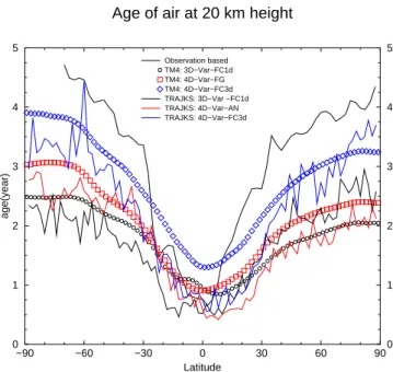
Fig. 4. The mean age of air, as a function of latitude, computed
with the TRAJKS trajectory model and the TM4 chemistry trans-port model (Meijer et al., 2004), and as derived from observations (Andrews et al., 2001).
In line with this, in Fig. 3 no discontinuity can be observed at the times of the annual discontinuity.
The sensitivity of the computed age to the exact defini-tion of crossing the tropopause is small. We imposed that the pressure of the trajectories should be at least 10% larger than the tropopause pressure for at least one day. The mean age decreased by 11 days (2%) if this criterion in the 4D-Var-FC3d experiment was omitted. Omitting the one-day crite-rion resulted in a decrease in mean age of 3 days.
The resulting mean ages of air as a function of latitude for the 3D-Var-FC1d, the 4D-Var-AN and the 4D-Var-FC3d experiments are shown in Fig. 4. The results of the corre-sponding runs with the TM4 model (Meijer et al., 2004) are shown here as well. The runs marked FC1d applied exactly the same data, apart from the pre-processing. FG denotes first guess, which is a 6h-forecast. The figure also shows the age of air derived from observations (Andrews et al., 2001). In the TM4-results the age in the extratropics of both hemispheres is larger for the 4D-Var-AN than for the 3D-Var-FC1d data. In the TRAJKS results the age in the south-ern hemisphere is larger for the 4D-Var-AN data, but in the northern hemisphere it is larger for the 3D-Var-FC1d data. Because the latter two differences nearly cancel, the 3D-Var-FC1d and 4D-Var-AN trajectory-based global mean ages of air are, as mentioned above, almost the same. However, the 4D-Var-based runs seem to reproduce the gradient between the tropics and the midlatitudes better than the 3D-Var based runs.
6 M. P. Scheele et al.: Trajectories-based age of air −90 −60 −30 0 30 60 90 Latitude 0 0 1 1 2 2 3 3 4 4 5 5 age(year)
Age of air at 20 km height
4D−Var−AN 4D−Var−FC3d 4D−Var−FC3d (july) Observation based
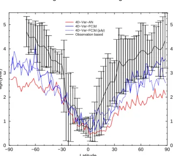
Fig. 5. The mean age of air, as a function of latitude, computed
with the TRAJKS trajectory model with different data sets and as observed. The black bars are standard deviations of the observa-tions.
In Fig. 5 the mean ages of all 4D-Var runs as well as the observation-based ages are shown as a function of latitude. The 4D-Var-FC3d ages are closest to the observations, but are still 0.5–1.5 year too small.
The 5-year backward trajectories were all started in the northern winter season, on 31 December. This may lead to a bias in the computed age of air, because the stratospheric meridional circulation has a seasonal cycle, with strongest transport during northern winter. Thus, the number of trajec-tories crossing the tropopause in the first months of the sim-ulation starting in northern hemispheric winter, December, is expected to be relatively large, leading to a somewhat smaller age of air. To investigate this effect, 5-year trajectories have been computed, using 4D-Var-FC3d data, with the same set-up as that for the other 5-year trajectories, but starting in July. Figure 5 shows that the run started in July, gives a larger age between the equator and 20◦N than the run started in De-cember. The weaker transport during northern hemispheric summer causes a larger mean age for the tropics in the run starting in July. In Fig. 3 we also can observe this seasonal dependency by comparing the two 4D-Var-FC3d runs. The computed mean age of air for these trajectories is 1.87 year, which is only slightly larger than the 1.84 year computed for the trajectories starting in December. As shown in Fig. 3, the larger age for the July-trajectories is mainly due to less intense transport in the first months of the simulation.
For all data sets the computed age of air in the extratropics is smaller than observed. Compared to the difference in age
between the results for the different data sets, the difference in age between the TRAJKS and the TM4 results is small. We tentatively conclude that the age of air in TM4 is not very sensitive to the noise introduced by the preprocessing. The effect of preprocessing might be largest near the equa-tor, where the age in the TM4 results is larger than in the TRAJKS results, and even larger than the observation-based age.
5 Conclusions
This study was motivated by results from a chemistry trans-port model (TM4), driven by ECMWF data, in which the simulated age of stratospheric air was much smaller than ob-served. As the ECMWF data are preprocessed before they drive the model, the question arose to what extent the sim-ulated age of air was influenced by this preprocessing. An-other question that was addressed is to what extent the esti-mates of the age of air depend on the type of forecast series of the data, in particular the forecast segment length.
We have integrated the trajectories for five years. By then, more than 90% of the trajectories started at 20 km had passed the tropopause (Fig. 3). For ages of more than five years we extrapolated the age distribution with an exponential decay function. This proved to be a reliable fit. As we used data of only one year, the results are not necessarily valid for other years. However, Meijer et al. (2004) found that the inter-annual variability is relatively small.
The results show that for the 3D-Var ERA-40 data the age is largest for forecast segments of 24 h. However, this age is still smaller than the age obtained from any of the applied 4D-Var data sets. For 4D-Var data the age is largest for 72-h forecast segments. This age, however, is still 0.5–1.5 year smaller than observed. We found that the difference between the age of air calculated with TM4 and TRAJKS is small compared to the differences resulting from different data sets. Thus, the effect of preprocessing in the TM4 on the age of air seems to be relatively small. Here it should be noted that in the case of TM4 quite some effort has been spent on reducing numerical noise in the calculation of mass fluxes for the TM4 model from the data during preprocessing (Bregman et al., 2003). Therefore this conclusion does not necessarily hold for other CTMs.
In the tropical stratosphere a computed larger age of air is not necessarily a more realistic age. Too much vertical trans-port might be compensated by erroneous horizontal transtrans-port of old air from the extratropical stratosphere. Such compen-sating errors are unlikely to occur in the age of air simulation for the extra-tropical stratosphere. Therefore our results sug-gest that the use of longer forecast segment lengths leads to a better description of the circulation.
A striking feature is that especially the 4D-Var data gen-erate more cross-tropopause transport, corresponding to a
smaller, less realistic age, when the horizontal resolution is increased.
We showed that it is sufficient to integrate trajectories over only about 5 years to estimate the mean age of air. Using forecast series of several days instead of analyses increases the estimated mean age of air. Applying TRAJKS instead of TM4 improves the latitudinal gradient at the edge of the tropical region. The underestimation of the mean age of air, encountered in the TM4 runs, is not due to the preprocessing as implemented for TM4. Of all runs the age derived from the 72-h forecast segments resembles the observations-based age of air most. We may conclude that the best choice to drive a CTM is using 4D-Var data with forecast segments with a length of several days. For ERA-40 data, using the last 24 h of 30-h forecast series is the best choice.
Acknowledgements. The authors thank an anonymous referee, A.
Stohl, and H. Wernli for their extensive comments, and T. van Noije and B. Bregman for inspiring discussions. We thank E. Meijer for making available the results of the TM4-runs. P. van Velthoven was partially supported by the EU Retro project EVK2-CT-2002-00170. Edited by: H. Wernli
References
Andrews, A. E., Boering, K. A., Dauble, B. C., Wofsy, S. C., Loewenstein, M., Jost, H., Podolske, J. R., Webster, C. R., Her-man, R. L., Scott, D. C., Flesch, G. J., Moyer, E. J., Elkins, J. W., Dutton, G. S., Hurst, D. F., Moore, F. L., Ray, E. A., Romashkin, P. A., and Strahan, S. E.: Mean ages of stratospheric air derived
from in situ observations of CO2, CH4, and N2O, J. Geophys.
Res., 106 (D23), 32 295–32 314, 2001.
Bregman, B., Segers, A., Krol, M., Meijer, E., and van Velthoven, P. F. J.: On the use of mass-conserving wind fields in chemistry-transport models, Atmos. Chem. Phys., 3, 447–457, 2003,
SRef-ID: 1680-7324/acp/2003-3-447.
Hall, T. M. and Plumb, R. A.: Age as diagnostic of stratospheric transport, J. Geophys. Res., 99 (D1), 1059–1070, 1994. Meijer, E. W., Bregman, B., Segers, A., and van Velthoven, P. F. J.:
The influence of data assimilation on the age of air calculated with a global chemistry-transport model using ECMWF wind fields, Geophys. Res. Lett., 31, doi:10.1029/2004GL021158, 2004.
Noije, T. P. C. van, Eskes, H. J., van Weele, M., and van Velthoven, P. F. J.: Implications of the enhanced Brewer-Dobson circula-tion in European Centre for Medium-Range Weather Forecasts reanalysis ERA-40 for the stratosphere-troposphere exchange of ozone in global chemistry transport models, J. Geophys. Res., 109, D19308, doi:10.1029/2004JD004586, 2004.
Scheele, M. P., Siegmund, P. C., and van Velthoven, P. F. J.: Sensi-tivity of trajectories to data resolution and its dependence on the starting point: in or outside a tropopause fold, Meteor. Appl., 3, 267–273, 1996.
Schoeberl, M. R., Douglass, A. R., Zhu, Z., and Pawson, S.: A comparison of the lower stratospheric age spectra derived from a general circulation model and two data assimilation systems, J. Geophys. Res., 108 (D3), 4113, doi:10.1029/2002JD002652, 2003.
Sigmond, M., Meloen, J., and Siegmund, P. C.: Stratosphere-troposphere exchange in an extratropical cyclone calculated with a Lagrangian method, Ann. Geophys., 18, 573–582, 2000,
SRef-ID: 1432-0576/ag/2000-18-573.
Simmons, A. J. and Gibson, J. K.: The 40 project plan, ERA-40 Project Rep. Series 1, 62 pp., 2000.
Stohl, A., Haimberger, L., Scheele, M. P., and Wernli, H.: An in-tercomparison of results from three trajectory models, Meteorol. Appl. 8, 127–135, 2001.
Stohl, A., Cooper, O. R., and James, P.: A Cautionary Note on the Use of Meteorological Analysis Fields for Quantifying Atmo-spheric Mixing, J. Atmos. Sci., 61, 1446–1453, 2004.
Tan, W. W., Geller, M. A., Pawson, S., and da Silva, A.: A case study of excessive subtropical transport in the stratosphere of a data assimilation system, J. Geophys. Res., 109, D11102, doi:10.1029/2003JD004057, 2004.
Weaver, J. C., Douglass, A. R., and Rood, R. B.: Thermodynamic balance of three-dimensional stratospheric winds derived from a data assimilation procedure, J. Atmos. Sci., 50, 2987–2293, 1993.
Wild, O., Sundet, J. K., Prather, M. J., Isaksen, I. S. A., Aki-moto, H., Browell, E. V., and Oltmans, S. J.: Chemical transport model ozone simulations for spring 2001 over the western Pa-cific: Comparison with TRACE-P lidar, ozonsondes, and Total Ozone Mapping Spectrometer columns, J. Geophys. Res., 108 (D21), 8826, doi:10.1029.2002JD003283, 2003.