The impact of mid-latitude intrusions into the polar vortex on ozone loss estimates

HAL Id: hal-00295248

https://hal.archives-ouvertes.fr/hal-00295248

Submitted on 3 Apr 2003

HAL is a multi-disciplinary open access

archive for the deposit and dissemination of

sci-entific research documents, whether they are

pub-lished or not. The documents may come from

teaching and research institutions in France or

abroad, or from public or private research centers.

L’archive ouverte pluridisciplinaire HAL, est

destinée au dépôt et à la diffusion de documents

scientifiques de niveau recherche, publiés ou non,

émanant des établissements d’enseignement et de

recherche français ou étrangers, des laboratoires

publics ou privés.

The impact of mid-latitude intrusions into the polar

vortex on ozone loss estimates

J.-U. Grooß, R. Müller

To cite this version:

J.-U. Grooß, R. Müller. The impact of mid-latitude intrusions into the polar vortex on ozone loss

estimates. Atmospheric Chemistry and Physics, European Geosciences Union, 2003, 3 (2), pp.395-402.

�hal-00295248�

www.atmos-chem-phys.org/acp/3/395/

Chemistry

and Physics

The impact of mid-latitude intrusions into the polar vortex on ozone

loss estimates

J.-U. Grooß and R. M ¨uller

Institut f¨ur Chemie und Dynamik der Geosph¨are I: Stratosph¨are (ICG-I), Forschungszentrum J¨ulich, J¨ulich, Germany Received: 5 November 2002 – Published in Atmos. Chem. Phys. Discuss.: 16 December 2002

Revised: 13 March 2003 – Accepted: 19 March 2003 – Published: 3 April 2003

Abstract. Current stratospheric chemical model simulations

underestimate substantially the large ozone loss rates that are derived for the Arctic from ozone sondes for January of some years. Until now, no explanation for this discrepancy has been found. Here, we examine the influence of intrusions of mid-latitude air into the polar vortex on these ozone loss es-timates. This study focuses on the winter 1991/92, because during this winter the discrepancy between simulated and ex-perimentally derived ozone loss rates is reported to be the largest. Also during the considered period the vortex was disturbed by a strong warming event with large-scale intru-sions of mid-latitude air into the polar vortex, which is quite unusual for this time of the year. The study is based on sim-ulations performed with the Chemical Lagrangian Model of the Stratosphere (CLaMS). Two methods for determination the ozone loss are investigated, the so-called vortex average approach and the Match method. The simulations for Jan-uary 1992 show that the intrusions induce a reduction of vor-tex average ozone mixing ratio corresponding to a system-atic offset of the ozone loss rate of about 12 ppb per day. This should be corrected for in the vortex average method. The simulations further suggest, that these intrusions do not cause a significant bias for the Match method due to effective quality control measures in the Match technique.

1 Introduction

It is difficult to determine the chemical ozone loss in the Arc-tic stratosphere because chemical ozone loss is masked by dynamic variability caused by reversible vertical and hor-izontal advection and by mixing of air masses. Different methods are known to derive the chemical ozone loss from observations such as a comprehensive set of ozone sonde measurements (Harris et al., 2002). Here we discuss the

Correspondence to: J.-U.Grooß (j.-u.grooss@fz-juelich.de)

so called vortex average method (Knudsen et al., 1998; EU, 2001) and the Match technique (von der Gathen et al., 1995; Rex et al., 1998). Both methods use ozone sonde data to-gether with meteorological analyses and estimates of the di-abatic descent to derive chemical ozone loss for the polar vortex. Briefly, the vortex average approach calculates the average of all vortex ozone data on an isentropic surface as a function of time. Using a correction for diabatic descent, the chemical ozone loss is derived. The Match method uses pairs of observations in the same air mass at different times, so called matches. These matches are determined by trajec-tory calculations on the basis of meteorological analyses and estimates of the diabatic descent. A statistical analysis is con-ducted to deduce the rate of ozone loss in the vortex from such a dataset. Only matches for which the distance between the positions of the air parcel trajectory and the second obser-vation is below the so-called Match radius (typically 500 km) contribute to the analysis. A selection procedure based on pa-rameters like the local vertical ozone gradient and the disper-sion of trajectory clusters is used to avoid matches in regions with high wind shear and non-homogeneous ozone distribu-tions.

During January in some years, large discrepancies were found between Match and the corresponding simulated ozone depletion rates (Becker et al., 1998, 2000; Kilbane-Dawe et al., 2001; Rex et al., 2003): For example, in 1992 the Match results for January 24±7 days yield ozone loss rates of 10.0±1.3 ppb/sunlight hour (54±7 ppb/day) whereas the corresponding box model simulations yield only 3.3±0.2 ppb/sunlight hour (18±1 ppb/day). Becker et al. (1998) further demonstrated that this discrepancy cannot be explained by known model uncertainties. Rex et al. (2003) show that this is the largest discrepancy of all the Match campaigns between 1992 and 2000: to explain the ozone loss rates in January 1992 with standard photochemistry the amount of active chlorine must exceed the maximum avail-able chlorine Cly by a factor of 2.5. They show by

statis-396 J.-U. Grooß and R. M¨uller: Impact of vortex intrusions on ozone loss estimates tical analyses of the Match data that the ozone loss must

have taken place during daylight and not during dark hours. They speculate that an unknown photochemical process that is very efficient at high solar zenith angles around 90◦may be responsible for this unknown ozone depletion, but up un-til now, no concrete mechanism has been proposed to our knowledge. These large January ozone loss rates seem to occur only during winters with stratospheric temperatures in January low enough to form a significant amount of PSCs.

The air masses within the polar vortex in early winter are often viewed as well isolated from mid-latitudes. However, this assumption is not true in in all winters at all times. Plumb et al. (1994) show an example of a large-scale intrusion of mid-latitude air masses into the polar vortex in January 1992. Here, we use simulations of the Chemical Lagrangian Model of the Stratosphere (CLaMS) (McKenna et al., 2002a,b) to investigate the impact of such intrusions in January 1992 on ozone loss estimates. At this time both large scale intrusions took place (Plumb et al., 1994) and the largest discrepancy between Match and model was found (Rex et al., 2003).

2 Model simulations

The Chemical Lagrangian Model of the Stratosphere (CLaMS) is described in detail by McKenna et al. (2002a,b). The simulation was performed for the 475 K potential tem-perature level for the time period between 12 January and 4 February 1992. The horizontal resolution is 90 km be-tween 30◦ and 90◦N and 450 km south of 30◦N corre-sponding to approximately 18 000 air parcels. Mixing be-tween air parcels is induced when the Lyapunov coefficient

λexceeds the critical value of 1.5 using a mixing time step of 12 h (see McKenna et al., 2002a; Konopka et al., 2002, for details). Wind and temperature information was taken from ECMWF data with high spatial and temporal resolution (1.125◦×1.125◦, 6 h). This model setup was successfully validated using a variety of data sets including satellite data from CRISTA (McKenna et al., 2002a), HALOE (Konopka et al., 2003), MLS and ILAS (McKenna et al., 2002b), and in situ data from the ER-2 aircraft (Grooß et al., 2002; Konopka et al., 2002) and ozone sondes (McKenna et al., 2002b).

For the problem under investigation, a two-dimensional isentropic simulation is justified, because the simulation pe-riod is rather short (23 days). To estimate the amount of di-abatic descent that the air parcels would have experienced, 16 600 3-D trajectories were calculated (without mixing) for the simulation period. The diabatic descent was calculated by a radiation scheme (Morcrette, 1991; Zhong and Haigh, 1995) using a 10-year climatology of HALOE ozone data as input (Grooß et al., manuscript in preparation). For this estimate, temperature and wind data were taken from the UKMO analyses that cover the complete stratosphere up to 0.3 hPa. The derived amount of descent for air parcels in the vortex is 21.5±2.4 K(1σ ) in 23 days which is less than

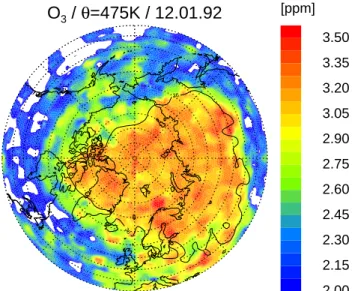
O

/

θ

=475K / 12.01.92

Fig. 1. Initialization for ozone on the 475 K level derived from

MLS data. White areas indicate mixing ratios below 2.0 ppm. Also plotted is the PV contour of 36 PVU that is employed here as the definition of the vortex edge.

1 km. In the two-dimensional isentropic simulation we do not simulate the exact positions of the air parcels correctly because of the neglect of diabatic descent. Thus, an exact sampling of the Match trajectories within the model domain as by Kilbane-Dawe et al. (2001) can not be performed here. However, the simulation still demonstrates the effect of the vortex intrusions very clearly.

To derive an initial ozone field at 475 K for the CLaMS simulation, we used version 5 data from the Microwave Limb Sounder (MLS) on board the Upper Atmosphere Research Satellite (UARS) (Barath et al., 1993) between 8 and 13 Jan-uary. Using backward and forward trajectories, the locations of the observations were mapped to the assimilation time (12 January 1992, 12:00 UT). These data were then combined on a regular grid with 1◦latitude×3◦ longitude spacing. Each grid point summarizes all data points within a distance less than 220 km using a cosine-square weighting with 110 km distance half-width. Figure 1 shows the derived ozone mix-ing ratio. The other species are initialized usmix-ing the Mainz photochemical 2-D model (Gidel et al., 1983; Grooß, 1996) mapped onto equivalent latitude.

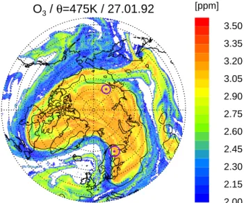
Figures 2 and 3 show examples of the simulated ozone mixing ratio for 22 and 27 January on a stereographic pro-jection. For illustration, they also show the location of two Match trajectories with over 0.5 ppm diagnosed ozone loss and over 50 sunlight hours (violet symbols). On 22 January, a large extended area of air masses outside the vortex between Scandinavia and Greenland with ozone mixing ratios below about 2.5 ppmv (blue colors) is visible. These air masses are drawn into the vortex as also simulated by Plumb et al. (1994). They can be seen as green colors over Newfoundland

O

/

θ

=475K / 22.01.92

Fig. 2. Simulated ozone mixing ratio for 22 January. The violet

stars and circles show the location and Match radius of two indi-vidual Match trajectories. The black contour corresponds to the 36 PVU line which is used here as the definition of the vortex edge. White areas indicate ozone mixing ratios below 2 ppm.

O

/

θ

=475K / 27.01.92

Fig. 3. As Fig. 2, but for 27 January.

and eastward of Greenland on 27 January. The simulations show that with time the intruded air masses are deformed and elongated. In this context it is important that the horizontal scale of intruded air masses shrinks within one week below about 500 km which is the maximum allowed Match radius. Figures 2 and 3 also show the individual Match radii of se-lected Match trajectories (≈300 km) as violet circles. The impact on the Match analysis is discussed below. On 27 Jan-uary, a second tongue of air around 75◦N, 180◦E starts to be drawn into the vortex.

1.0 1.5 2.0 2.5 3.0 3.5 ppm O3 [Sonde] 1.0 1.5 2.0 2.5 3.0 3.5 ppm O 3 [CLaMS] inside vortex outside vortex

Fig. 4. Comparison of ozone mixing ratio obtained from 123 ozone

sondes between 17 and 31 January 1992 with CLaMS simulation interpolated onto the sonde location on the 475 K level.

Figure 4 shows an intercomparison of the simulation with ozone data obtained from 123 sondes from all stations in-volved in the EASOE campaign between 17 and 31 January. Observations within the polar vortex are shown as red circles while the others are shown as blue circles. The agreement between the CLaMS simulation and the observation seems reasonable for the purpose of this study. The CLaMS sim-ulation is able to reproduce reasonably the variability of ob-served ozone mixing ratios both inside and outside the vor-tex. Some outliers especially with low observed ozone mix-ing ratios could not be reproduced by the simulation. The reason for these discrepancies may likely be the uncertainty of the initialization that was based on MLS data.

From Figs. 2 to 4 it is evident that the ozone mixing ratios in the polar vortex are not necessarily distributed uniformly on a potential temperature surface. Ozone variability within the polar vortex exists because of various reasons. In spring 1997, for example, a particularly pronounced inhomogene-ity of ozone depletion within the polar vortex was both ob-served and simulated (M¨uller et al., 1997; Schulz et al., 2000; McKenna et al., 2002b; Tilmes et al., 2003). Also inhomo-geneous diabatic descent and intrusions at earlier times that have not yet been completely mixed with vortex air are pos-sible reasons for variability of ozone inside the vortex on an isentropic surface.

3 Comparison with the vortex average approach

Principally the ozone variability itself should not signifi-cantly influence estimates of vortex averaged ozone loss in a confined vortex except that it increases the statistical error of the result. However, intrusions of a significant amount of air from mid-latitudes into the vortex cause a systematic off-set of averaged ozone mixing ratios. Since the

vortex-398 J.-U. Grooß and R. M¨uller: Impact of vortex intrusions on ozone loss estimates

Vortex average (PV>36PVU,

θ

=475K)

20.01.92 01.02.92 2.95 3.00 3.05 3.10 3.15 O3 [ppm] O₃ Tracer 20.01.92 01.02.92 0 5 10 15 20 O3

Loss Rate [ppb/day]

O₃

Tracer

Fig. 5. Vortex average of the simulations. The top panel shows the

vortex average ozone mixing ratio (blue line) and the average pas-sively advected tracer that was initialized identically as ozone (red line). The bottom panel shows the time derivative of the top panel, i.e. the ozone (or tracer) change per day for ±2.5 day intervals. The vortex edge is assumed to be at a constant value of 36 PVU.

average method depends on the assumption that the vortex air masses are well isolated from mid-latitudes, it should show a bias in the derived ozone loss rate during a time period with vortex intrusions. In mid-January 1992, the ozone mixing ra-tios below potential temperature levels of ≈500 K are lower outside the vortex than inside and vice versa above. Thus, the intrusions into the polar vortex would lead to an overesti-mate of chemical ozone depletion detected by this method at the 475 K level that is discussed here. Some studies employ-ing the vortex-average method try to correct for cross vortex edge transport by trajectory simulations, e.g. Knudsen et al. (1998) find no significant effect in the year 1997. However, that is clearly not true for other winters, especially for the winter 1991/92 discussed here.

Here, we can use the CLaMS simulation to quantify the bias that results from the intrusions. To derive the chemical ozone depletion comparable to the vortex average approach, only the average ozone mixing ratio of all airparcels within the polar vortex must be calculated. These results depend

Vortex average (Nash et al. ,

θ

=475K)

20.01.92 01.02.92 3.00 3.05 3.10 3.15 O3 [ppm] O₃ Tracer 20.01.92 01.02.92 −5 0 5 10 15 20 O3

Loss Rate [ppb/day]

O3

Tracer

Fig. 6. As Fig. 5, but for a different definition of the vortex edge.

Here the definition by Nash et al. (1996) was used.

clearly on the definition of the vortex edge. Here we use the same definition that is used in the Match analyses Rex et al. (1998), i.e. the 36 PVU line from ECMWF data on the 475 K level. Figure 5a shows the ozone mixing ratio averaged over the vortex area defined in this way for the time of this simu-lation as a blue line. The red line shows the vortex average of a passive tracer that was initialized identically to the ozone mixing ratio. As the tracer is not influenced by chemistry, its vortex average should be constant with time. However, from this analysis it is evident that in January 1992, the major frac-tion of the change in the vortex average ozone mixing ratio is due to the dynamically caused intrusions into the vortex but not due to chemical ozone depletion. The change of the dynamical ozone tracer in this simulation is a measure for the bias in derived chemical ozone depletion. To derive the chemical ozone loss, one should correct for this dynamical effect. Figure 5b shows the time derivative of the vortex av-erage ozone mixing ratio including chemical ozone loss (blue line) and the passive ozone tracer mixing ratio (red line) for

±2.5 days, i.e. for intervals of 5 day length. The time deriva-tive of the passive ozone tracer (red line) can be viewed as the bias of derived ozone depletion rates due to vortex intru-sions. Around 24 January, this dynamical bias is about 11 to

36 36 0 5 10 15 20 Longitude 54 56 58 60 62 Latitude

Fig. 7. Sketch of the “virtual Match” calculation. The green line

corresponds to one example trajectory ending at the large green cir-cle. The Match radius here is 300 km indicated by the red circir-cle. 8 new locations are marked by the red circles for which only those inside the vortex (filled circles) are considered. The vortex edge is plotted as a thick black line. Grey circles correspond to the individ-ual CLaMS air parcel locations and those chosen for the Match are marked blue.

14 ppb/day.

The bias derived from vortex-averaged ozone tracer de-pends also on the definition of the vortex edge. If the vortex edge is moved poleward by using a greater PV value, the derived ozone depletion rate is lower and vice versa (e.g.

≈8 ppb/day for PVedge = 40 PVU and ≈24 ppb/day for PVedge=30 PVU on 24 January). However, the general pat-terns of Fig. 5 do not change significantly. In some studies, a time-dependent definition of the vortex edge is used defined by the maximum PV gradient after Nash et al. (1996). The results with this definition are comparable and are shown in Fig. 6. in spite of the high day-to-day variability caused by the variability in the calculated vortex area, the general shape of ozone loss and loss rates for the two vortex edge defini-tions does look similar, and thus the conclusions drawn do not change.

4 Comparison with the Match approach

The Match method is a more sophisticated approach than the vortex average method. It aims at avoiding such errors as dis-cussed above since individual air parcels are examined that have been probed twice by an ozone sonde inside the vortex. It is therefore unlikely that earlier vortex observations match with air masses that have crossed the vortex edge during the time of the Match trajectory. However, there are displace-ments between the probed air mass and the location of the matching air mass given by the Match radius and furthermore by uncertainties induced by the trajectory calculation.

As has been shown above by the CLaMS simulation, the large-scale intrusions in 1992 caused filaments with a width below the maximum Match radius of 500 km within about one week. Therefore, the systematic offset described above may also influence the Match results, however, to a lesser ex-tent. In order to quantify the expected impact of these vortex intrusions on the Match results, an additional “virtual Match” simulation was performed. Figure 7 illustrates this method: At each CLaMS air parcel within the polar vortex on one day a trajectory (green line) was started to predict the location of the air parcel on a later day (large green circle). For each of the calculated locations, 8 new points were determined with the distance of a given Match radius equally distributed in all directions (red circles). If a new point is still within the vor-tex, it was considered a match with the first air parcel. The corresponding passive ozone tracer mixing ratios were then determined from the CLaMS simulation using the data from the closest CLaMS point (blue circles) to each new point. The average vortex ozone depletion rate was then determined from these matches exactly as in the Match analyses.

In the Match approach there are quality measures to avoid matches in regions with possible inhomogeneous ozone mix-ing ratio distribution. Only those trajectories that fulfill these criteria are selected for matches. This simulation is well suited to quantify how these trajectory selection criteria work. Therefore, the effect of two of these selection criteria has been investigated by the virtual Match method: Firstly, the “PV criterion” selects only those trajectories along which PV does not change significantly. In detail, only those trajec-tories are selected in which the PV value is always within 25% of the average PV value along the trajectory. Secondly, the “cluster trajectory criterion” is determined by calculating for each trajectory a cluster of trajectories starting at close locations. In detail, 4 trajectories start with 100 km distance (north, south, west and east) on the same potential tempera-ture level and 2 trajectories ±5 K above and below this level. Only those trajectories are chosen, that stay within 1200 km and 1300 km for the 4 and 2 trajectories, respectively. A third criterion used in the Match method depends on the vertical structure of the ozone sonde data and is therefore not consid-ered by this virtual Match simulation.

Here, the trajectory length was chosen to be 4 days from 22 January to 26 January, which is the average trajectory length for the trajectories contributing to the Match results on 24 January. The chosen Match radius was 300 km. The results are summarized in Table 1 for the use of different trajectory selection criteria.

If no selection criterion is used, 3717 trajectories were started within the vortex of which 2970 stayed within the vortex over the 4 day period resulting in 21 404 virtual Match events.

As above, the ozone loss rate bias was also determined from the passive ozone tracer from which the (passive) ozone depletion rate was derived exactly as in the Match analy-sis. The resulting bias was 2.40±0.07 ppb per sunlight hour

400 J.-U. Grooß and R. M¨uller: Impact of vortex intrusions on ozone loss estimates

Table 1. Summary of the results for the “virtual Match” simulation for 4-day trajectories and a match radius of 300 km. The Table columns

show the results employing different selection criteria. Details see text

Selection Criteria None PV Cluster Traj. Both

Number of Trajectories 3717 1998 2866 1726

Virtual Matches 21404 14434 17716 12544

Ozone Loss Rate Bias

(ppb/sunlight h) 2.40 ±0.07 –0.41±0.08 –0.23±0.07 –0.67±0.09 Subset of 20 Matches

(ppb/sunlight h) 2.41 ±2.72 –0.30±2.57 –0.12±2.56 –0.54±2.66

(12.1±0.4 ppb perday) that is comparable to what was de-termined for the vortex average method for this time frame. This result does not seem to depend strongly on the cho-sen Match radius, e.g. for a Match radius of 450 km, the ozone depletion rate derived from the passive ozone tracer is 13.8±0.4 ppb per day.

Clearly, the use of the selection criteria has a significant influence on the resulting ozone loss rate bias. The applied selection criteria do indeed sort out trajectories that are in-fluenced by inhomogeneities: As summarized in Table 1, the derived bias is even slightly negative, if a selection criterion is applied, regardless whether the PV criterion only, the clus-ter trajectory criclus-terion only or both criclus-teria are applied. This clearly shows that it is adequate and necessary for the Match analysis to use these selection criteria in order to avoid the biases examined here.

The Match results also depend on the sampling of the po-lar vortex achieved by the Match trajectories. In the Match analysis for 24 January 1992, there are only 19 Match events. With this simulation we also tested what statistical error one should expect from this number of events. This was done by randomly choosing a subset of 20 matches out of all virtual matches which was repeated 200 000 times for each choice of trajectory selection criteria. From each subset of 20 matches the ozone depletion rate is evaluated exactly as in the regu-lar Match analysis. Figure 8 shows histograms of the derived ozone loss rate bias for subsets of 20 matches for no selection criterion (red) and both selection criteria (blue). The average and 1σ standard deviation of these histograms are shown in the bottom row of Table 1. The standard deviation of the so derived results for all choices of trajectory selection criteria is around 2.6 ppb per sunlight hour which is a factor 2 greater than the reported Match error bar for 24 January (Rex et al., 1998).

Further uncertainties could arise from the uncertainties in the wind data. However, the Match trajectory errors due to uncertainties in the wind data can not be examined by this simulation since both the simulation and the Match trajectory calculation are based on the same meteorological analyses (ECMWF).

−10 −5 0 5 10

Ozone loss rate bias [ppb/sunlight hour] 0 2000 4000 6000 8000 10000 12000

Number of subsets (20 Matches)

Selection Criteria:

None

PV & Cluster Traj.

Fig. 8. Histogram of the derived ozone loss rate bias for 200 000

subsets of 20 out of all virtual matches. The results for the case that no trajectory selection criterion is applied are plotted as red lines. The case that both trajectory selection criteria are applied are plotted as blue lines. The dashed vertical lines show the ozone loss rate bias derived from the passive ozone tracer for all virtual matches. The red dotted line shows the discrepancy between simulation and Match after Becker et al. (1998).

5 Conclusions

We have shown that intrusions of mid-latitude air into the polar vortex introduce a systematic offset of vortex average ozone mixing ratios. Estimates of ozone loss rates are influ-enced by this effect. In January 1992, the resulting ozone de-pletion rate bias due to intrusions was estimated to be about 11 to 14 ppb per day for the vortex average method. Since the large-scale intrusions reached horizontal dimensions be-low the Match radius, their potential influence on the Match results was investigated. The model simulations show that these intrusions should not influence the ozone depletion rate derived from the Match analysis, if the usual trajectory selec-tion criteria are applied.

Furthermore, it was shown for January 1992 that the pub-lished 1σ uncertainty on the basis of 19 matches is

estimated by a factor of 2 due to the sparse sampling of the polar vortex and the ozone variability within the polar vortex. However, even with this larger uncertainty, the published dis-crepancy between Match deduced ozone loss rates and those derived from model simulations cannot be explained. Acknowledgements. The authors thank Peter von der Gathen, Markus Rex and other participants of a workshop on stratospheric ozone loss in Potsdam in March 2002 for fruitful discussions. We thank the referees for their valuable suggestions. We acknowledge the MLS team led by Joe Waters. We also thank the European Cen-tre for Medium-Range Weather Forecasts and the United Kingdom Meteorological Office for providing meteorological analyses.

References

Barath, F. T., Chavez, M. C., Cofield, R. E., Flower, D. A., Frerking, M. A., Gram, M. B., Harris, W. M., Holden, J. R., Jarnot, R. F., Kloezeman, W. G., Klose, G. J., Lau, G. K., Loo, M. S., Mad-dison, B. J., Mattauch, R. J., McKinney, R. P., Peckham, G. E., Pickett, H. M., Siebes, G., Soltis, F. S., Suttie, R. A., Tarsala, J. A., Waters, J. W., and Wilson, W. J.: The Upper Atmosphere Research Satellite microwave limb sounder instrument, J. Geo-phys. Res., 98, 10 751–10 762, 1993.

Becker, G., M¨uller, R., McKenna, D. S., Rex, M., and Carslaw, K. S.: Ozone loss rates in the Arctic stratosphere in the winter 1991/92: Model calculations compared with Match results, Geo-phys. Res. Lett., 25, 4325–4328, 1998.

Becker, G., M¨uller, R., McKenna, D. S., Rex, M., Carslaw, K. S., and Oelhaf, H.: Ozone loss rates in the Arctic stratosphere in the winter 1994/1995: Model simulations underestimate results of the Match analysis, J. Geophys. Res., 105, 15 175–15 184, 2000. EU: European research in the stratosphere 1996-2000, chap. 3.5,

pp. 112–117, EUR 19867, Brussels, 2001.

Gidel, L. T., Crutzen, P. J., and Fishman, J.: A two-dimensional photochemical model of the atmosphere; 1: Chlorocarbon emis-sions and their effect on stratospheric ozone, J. Geophys. Res., 88, 6622–6640, 1983.

Grooß, J.-U.: Modelling of Stratospheric Chemistry based on HALOE/UARS Satellite Data, PhD thesis, University of Mainz, 1996.

Grooß, J.-U., G¨unther, G., Konopka, P., M¨uller, R., McKenna, D. S., Stroh, F., Vogel, B., Engel, A., M¨uller, M., Hoppel, K., Bevilacqua, R., Richard, E., Webster, C. R., Elkins, J. W., Hurst, D., Romashkin, P. A., and Baumgardner, D. G.: Simulation of ozone depletion in spring 2000 with the Chemical Lagrangian Model of the Stratosphere (CLaMS), J. Geophys. Res., pp. 8295, doi:10.1029/2001JD000 456, 2002.

Harris, N., Rex, M., Knudsen, B., Manney, G., M¨uller, R., and von der Gathen, P.: Comparison of empirically derived ozone loss rates in the Arctic vortex, J. Geophys. Res., 107, doi:10.1029/2001JD000 482, 2002.

Kilbane-Dawe, I., Harris, N., Pyle, J., Rex, M., Lee, A., and Chip-perfield, M.: A comparison of Match and 3D model ozone loss rates in the Arctic polar vortex during the winters of 1994/95 and 1995/96, J. Atmos. Chem., 39, 123–138, 2001.

Knudsen, B. M., Larsen, N., Mikkelsen, I. S., Morcrette, J.-J., Braa-then, G. O., Kyr¨o, E., Fast, H., Gernandt, H., Kanzawa, H., Nakane, H., Dorokhov, V., Yushkov, V., Hansen, G., Gil, M.,

and Shearman, R. J.: Ozone depletion in and below the Arctic vortex for 1997, Geophys. Res. Lett., 25, 627–630, 1998. Konopka, P., Grooß, J. U., G¨unther, G., McKenna, D. S., M¨uller,

R., Elkins, J. W., Fahey, D., Popp, P., and Stimpfle, R. M.: Weak influence of mixing on the chlorine deactivation dur-ing SOLVE/THESEO2000: Lagrangian Modeldur-ing (CLAMS) versus ER-2 in situ observations, J. Geophys. Res., 108, doi:10.1029/2001JD000 876, 2002.

Konopka, P., Grooß, J. U., Bausch, S., M¨uller, R., McKenna, D. S., Morgenstern, O., and Orsolini, Y.: Dynamics and chemistry of vortex remnants in late Arctic spring 1997 and 2000: Simula-tions with the Chemical Lagrangian Model of the Stratosphere (CLaMS), Atmos. Chem. Phys. Discuss., 3, 1051–1080, 2003. McKenna, D. S., Konopka, P., Grooß, J.-U., G¨unther, G., M¨uller,

R., Spang, R., Offermann, D., and Orsolini, Y.: A new Chem-ical Lagrangian Model of the Stratosphere (CLaMS): Part I Formulation of advection and mixing, J. Geophys. Res., 107, doi:10.1029/2000JD000 114, 2002a.

McKenna, D. S., Grooß, J.-U., G¨unther, G., Konopka, P., M¨uller, R., Carver, G., and Sasano, Y.: A new Chemical Lagrangian Model of the Stratosphere (CLaMS): Part II Formulation of chemistry-scheme and initialisation, J. Geophys. Res., 107, doi:10.1029/2000JD000 113, 2002b.

Morcrette, J.-J.: Radiation and cloud radiative properties in the Eu-ropean Centre for Medium-Range Weather Forecasts forecasting system, J. Geophys. Res., 96, 9121–9132, 1991.

M¨uller, R., Grooß, J.-U., McKenna, D., Crutzen, P. J., Br¨uhl, C., Russell, J. M., and Tuck, A. F.: HALOE observations of the ver-tical structure of chemical ozone depletion in the Arctic vortex during winter and early spring 1996–1997, Geophys. Res. Lett., 24, 2717–2720, 1997.

Nash, E. R., Newman, P. A., Rosenfield, J. E., and Schoeberl, M. R.: An objective determination of the polar vortex using Ertel’s po-tential vorticity, J. Geophys. Res., 101, 9471–9478, 1996. Plumb, R. A., Waugh, D. W., Atkinson, R. J., Newman, P. A., Lait,

L. R., Schoeberl, M. R., Browell, E. V., Simmons, A. J., and Loewenstein, M.: Intrusions into the lower stratospheric Arctic vortex during the winter of 1991–1992, J. Geophys. Res., 99, 1089–1105, 1994.

Rex, M., von der Gathen, P., Harris, N. R. P., Lucic, D., Knud-sen, B. M., Braathen, G. O., Reid, S. J., De Backer, H., Claude, H., Fabian, R., Fast, H., Gil, M., Kyr¨o, E., Mikkelsen, I., Rum-mukainen, M., Smit, H. G., St¨ahelin, J., Varotsos, C., and Za-itcev, I.: In situ measurements of stratospheric ozone depletion rates in the Arctic winter 1991/92: A Lagrangian approach, J. Geophys. Res., 103, 5843–5853, 1998.

Rex, M., Salawitch, R. J., Santee, M. L., Waters, J. W., Hoppel, K., and Bevilacqua, R.: On the unexplained stratospheric ozone losses during cold Arctic Januaries, Geophys. Res. Lett., 30, 1008, doi:10.1029/2002GL016 008, 2003.

Schulz, A., Rex, M., Steger, J., Harris, N. R. P., Braathen, G. O., Reimer, E., Alfier, R., Beck, A., Alpers, M., Cisneros, J., Claude, H., De Backer, H., Dier, H., Dorokhov, V., Fast, H., Godin, S., Hansen, G., Kanzawa, H., Kois, B., Kondo, Y., Kosmidis, E., Kyr¨o, E., Litynska, Z., Molyneux, M. J., Murphy, G., Nakane, H., Parrondo, C., Ravegnani, F., Varotsos, C., Vialle, C., Viatte, P., Yushkov, V., Zerefos, C., and von der Gathen, P.: Match ob-servations in the Arctic winter 1996/97: High stratospheric ozone loss rates correlate with low temperatures deep inside the polar

402 J.-U. Grooß and R. M¨uller: Impact of vortex intrusions on ozone loss estimates

vortex, Geophys. Res. Lett., 27, 205–208, 2000.

Tilmes, S., M¨uller, R., Grooß, J.-U., McKenna, D., Russell, J., and Sasano, Y.: Calculation of chemical ozone loss in the Arctic winter 1996–1997 using ozone-tracer correlations: com-parison of ILAS and HALOE results, J. Geophys. Res., 108, doi:10.1029/2002JD002 213, 2003.

von der Gathen, P., Rex, M., Harris, N. R. P., Lucic, D., Knudsen, B. M., Braathen, G. O., De Backer, H., Fabian, R., Fast, H.,

Gil, M., Kyr¨o, E., Mikkelsen, I. S., Rummukainen, M., St¨ahelin, J., and Varotsos, C.: Observational evidence for chemical ozone depletion over the Arctic in winter 1991–92, Nature, 375, 131– 134, 1995.

Zhong, W. and Haigh, J. D.: Improved broadband emissivity param-eterization for water vapor cooling rate calculations, J. Atmos. Sci., 52, 124–138, 1995.