The design and construction of a 3-D scanner from off-the-shelf compnents

The Design and Construction of a 3-D

Scanner from Off-the-Shelf Components

By

Wandy Sae-Tan

Submitted to the

Department of Electrical Engineering and Computer Science In Partial Fulfillment of the Requirements for the

Degree of Master of Engineering in Electrical Engineering and Computer Science at the Massachusetts Institute of Technology

_May 27, 1998

Copyright 1998 WG7iidy Sae-Tan. All r iits reserved.

The author hereby grants to M.I.T. permission to reproduce and distribute publicly paper and electronic copies of this thesis and to grant others the right to do so.

Author

Department of El /ctrical Engineerin and Computer Science May 27, 1998

Certified by

-DI r. Amar Gupta ... es. ieup sor

Accepted by

Arthur C. Smith Chairman, Department Committee on Graduate Theses

MASSACHUSETTS INSTITUTE OF TECHIO- lOGY

JUL 141998

F

The Design and Constructor of a 3-D Scanner from Off-the-Shelf Components By

Wandy Sae-Tan

Submitted to the Department of Electrical Engineering and Computer Science

May 27, 1998

In Partial Fulfillment of the Requirements for the Degree of

Master of Engineering in Electrical Engineering and Computer Science

ABSTRACT

We present the design and prototype implementation of a low-cost 3-D scanning system using off-the-shelf personal computer, digital camera, and computer projector. In this system, we project a fixed grid onto the subject being scanned. By placing a camera at an angle, we can capture the distortions of the grid caused by the scanned subject. These horizontal distortions can then be converted into a collection of depth points. The precision and resolution of this system will not be comparable to those of existing laser scanners, but the affordability of this design could make it very attractive to an entirely new class of applications. Our prototype has served well as a "proof-of-concept". With further work, we believe it is possible to turn this design into a practical implementation.

Thesis Supervisor: Dr. Amar Gupta

TABLE OF CONTENT

1 INTRODUCTION 5

1.1 3-D Scanner from Off-the-Shelf Components 5

1.2 Project Scope 6

1.3 Paper Roadmap 6

2 BACKGROUND 7

2.1 Basic Approaches 7

2.2 Commercially Available Systems 8

3 DESIGN OVERVIEW 11

3.1 Considerations and Criteria 11

3.2 The Idea 11

3.3 Components 12

3.4 Assumptions 13

3.5 Scanning 14

3.6 Processing 15

4 QUANTIFYING GRID DISTORTIONS 17

4.1 The Goal 17

4.2 Extracting Intersections 17

4.3 Pixel Filter 19

4.4 Identify Intersections 23

5 CONVERTING DISTORTIONS TO DEPTHS 26

5.1 Optical Model 26

5.2 Model Verification 29

6 IMPLEMENTATION OVERVIEW 32

6.1 Setup And Functionality 32

6.2 Process Flow 33

7 DETAILS OF PROCESSING COMPONENTS 36

7.1 Image Subtractor 36

7.2 Intersection Extractor 36

7.3 Point Mapper 40

8 EVALUATION 43

8.1 Fulfillment of Design Goals 43

8.2 Accuracy 44

8.3 Robustness 45

8.4 Ease of Setup 46

48 48 49 9 CONCLUSION Future Work Summary 10 REFERENCES 11 APPENDICES 11.1 Class Prototype 11.2 Class PrototypeFrame 11.3 Class FilelO 11.4 Class FindPoint 11.5 Class GridPointProcessor 11.6 Class ImageProcessor 11.7 Class MapPoints 11.8 Class OpticCalculator 11.9 Class Pattern 11.10 Class PatternFilter 11.11 Class PatternParser 11.12 Class GridGenerator 11.13 Class GridGeneratorFrame 11.14 Class Square

1

INTRODUCTION

Have you ever heard of a disposable 3-D point-and-shoot camera?

No one has. The techniques for capturing two-dimensional data have been so well developed that a five-year old and pick up a $10 camera and shoot a picture. But when it comes to capturing three-dimensional objects, no one has figured out how to do it cheaply and with the quality that we see in photographs produced by an ordinary camera. This paper

attempts to address some of these concerns in the hope of bringing 3-D scanners one-step closer to the mainstream market.

The main concern addressed in this project is cost. 3-D scanners today are built from proprietary hardware and software, making them highly customizable to the buyer's specific needs. However, the high costs of these systems have limited their applications to the few domains that need realistic surface digitizing capability. What if we could build a 3-D scanner that is very low in cost and maintenance? Could people dream up applications for affordable 3-D data?

1.1 3-D SCANNER FROM OFF-THE-SHELF COMPONENTS

In this paper, we explore a possible design of a 3-D scanner from off-the-shelf components. We also present the results and evaluation of a prototype unit that we built based on the design: using a digital camera, a computer projector, and a personal computer.

How could this be done? We project a pre-determined grid onto the scanned subject, and observe the grid distortion through the digital camera. We then convert the horizontal discrepancies into depth information, which we can assemble to build a three-dimensional model.

The design is simple. The cost is low. But as our prototype implementation shows, it certainly has its share of limitations and problems. We will present the details of the system

1.2 PROJECT SCOPE

This project covers the following aspects of creating the 3-D scanning system: * Design of system setup and algorithms needed for processing

" Implementation of the processing algorithms and optic model that takes 2-D images

and produces 3-D (x, y, z) model file.

We decided to leave the following out of the project, because we feel that they are not essential for constructing our "proof-of-concept" system:

* Completely automated control of digital camera and computer projector. * Visualization of the 3-D model file.

1.3 PAPER ROADMAP

In this next chapter, we will provide background information on the field of three-dimensional scanning. We will describe the basic concepts and detail the state-of-the-art commercial systems. We will also discuss the advantages, limitations, and current applications of these scanning systems.

In Chapter 3, we will give a functional and design overview of our 3-D scanning system made from off-the-shelf components. We will describe how the system works from a high level point of view.

The next three chapters discuss different aspects of system design in detail. Chapter 4 covers the problem and solution to describing grid distortion in a quantitative manner. Chapter 5 shows the optical model and the mathematics needed to convert horizontal grid distortions into depth information.

Chapter 6 and 7 are devoted to the prototype implementation we have completed. We will first present the structure and flow of our processing application from a high level. Then, we will examine the implementation details of the individual software components.

Once we have completed the presentation of all the technical details of the system, we will present an in-depth evaluation of our efforts in Chapter 8. And finally, we will conclude the paper with Chapter 9, where we will present a summary and a few possibilities for future work that could be extended from this project. We have also included an appendix, which lists the source code for the prototype programs written to demonstrate the design.

2

BACKGROUND

The basic techniques for capturing three-dimensional information can be divided up into two groups: contact and non-contact. These approaches have their tradeoffs.

2.1.1 Contact

The contact approach is often referred to as "surface digitizing". It involves taking discrete points from a surface using touch trigger probe. This approach has some fundamental advantages over non-contact systems:

" Treatment of surfaces to prevent reflections is not required.

* Vertical faces can be accurately scanned.

* Data density is not fixed and is automatically controlled by the shape of the component.

* Time consuming manual editing of the data to remove stray points is not required. However, this approach can be very time-consuming, since the probe must be physically moved over the entire surface. For this reason, we ruled out the contact approach when designing our off-the-shelf components 3-D scanning system.

2.1.2 Non-contact

The non-contact approach is often referred to as "scanning". It typically involves emitting a light (laser or white light) onto the subject. The surface is recorded via the behavior of the lights. In the case of a laser-based scanner, a CCD screen is used to capture the reflectance of laser that bounces off the surface of the subject. There are also products that project modulated white light to capture 3-D data (see Section 2.2.2). The non-contact system offers the following advantages over mechanical contact-based systems:

* Since all that touches the model is a beam of light, the laser system allows fragile, delicate, and highly detailed surfaces to be scanned without damage.

* The model may be made of metal, wood, plastic, plaster, foam or even clay. * The data collected are true surface data without stylus offsets or deflection.

Since no mechanical movement is required, non-contact systems are usually faster

than its contact-based counterparts.

Non-contact systems also have their problems. The biggest drawback being that light beams

cannot reach all places of the subject, so often times a scan will have "shadow" regions or

"holes" where the light could not reach. These regions must be extrapolated from nearby

surfaces or filled-in manually. However, speed and ease of operation are important to the

design of our 3-D scanner, so we have adopted a non-contact design.

2.2

COMMERCIALLY AVAILABLE SYSTEMS

In this section we will introduce other companies and produces in the field of 3-D scanning.

The companies and products profile will put our project in a broader market context and

help us understand the current technologies and applications.

2.2.1

Cyberware

Cyberware (www.cyberware.com) manufactures a variety of standard and custom design instruments for three-dimensional scanning. Its most differentiating products are the head scanners and full body scanners (as shown in picture). Cyberware pioneered the techniques for scanning human faces, and extended 3-D applications from industrial design and manufacturing to anthropology

and entertainment. The head scanner produces a detailed three-dimensional data set of

facial features and a detailed texture map of the surface color. It has been used in special

effects production of Terminator II, Jurassic Park, and many other popular movies.

The full body scanner is a highly respectable product, aiming to bring 3-D scanning to an

even wider market. The scanner has four moving scanning heads that travels up and down

along the axis. A complete full-body scan is completed in 18 seconds (scan data processing

takes significantly longer, depending on the desired output). The scanner is a great

eye-catcher

-

spanning an area of 15'x15' and producing a 3-D scan on screen within a minute.

order of $250,000. Beyond the scanner, the buyer also needs to purchase high-end SGI

workstations to run the processing software, which can easy cost another tens and thousands

of dollars. The high cost of this scanner is in fact the inspiration for this project. Getting a

3-D scan is fun

-

wouldn't it be great if more people could afford to do it?

2.2.2

[TC]

[TC]

Inc. (www.tc2.com) is

member-driven organization aiming to create

innovative technical solutions to

enhance the future of apparel

manufacturing in the United States.

One of its projects under research and

development is a 3-D non-contact

full-length body measurement system.

The goal of this project is to develop a

kind of "automated tailor", capable of

measuring the human body in a snap-shol

custom-tailored clothes.

3DPdafa lpoj ld aed uday

n C a t

Zi; I

\ZE~

F and cea riauodal patlkiu

the information collected to produce

In the 3-D capture respect, the [Tq

system is functionally identical to the Cyberware full

body scanner. However, its approach to scanning is a unique departure from other scanner

systems. Instead of recording laser reflectance, [TC]

uses specially modulated white lights to

produce sinusoidal patterns on the scanned subject. Not using laser allows them to not have

any moving parts in the system to scan a large subject. It also brings down the cost to less

than 1/2 of the Cyberware scanner. The figure above shows a high-level functional view of

the system. If [TC]

successfully develops versions of this product with a smaller footprint

and lowers the cost of light modulation components, you could be finding one of these

systems at an apparel store near you.

2.2.3

Digibotics

Digibotics (www.digibotics.com) manufactures a variety of advanced laser-based 3-D

scanners, specializing in engineering design, rapid prototyping, modeling, and animation. Its

most differentiating technology is its adaptive scanning algorithm. The figure on the next

page demonstrates the workings of this algorithm. In the picture, we are looking at the

object being scanned from above. The scanned objects are the four cylinders (appear as

_11111111111111 ~XIIII~XIIWIII I~

circles in the picture). The red lines are the laser beams generated by the algorithms to complete the

scanning of the subject. Adaptive scanning algorithm allows the scanner to measure points in

the deepest cavities and completely eliminates the shadowing effects normally found on other scanning systems. This adaptive scanning technique truly takes advantage of the fact that laser emitters can be actively controlled in a closed setting. Such techniques to remove "shadows" will be very ditticult to implement in our orr-mte-snelr

component design, since we have a single light source whose location can not be easily adjusted.

2.2.4 Faro Technologies

Faro Technologies (www.faro.com) develops of portable and precise measurement solutions. Its multi-axis, articulated arms along with a CAD-based measurement software program provide 3D solutions for a variety of manufacturing and design applications. It uses probes to digitize the

surface by contact. Its leading product,

FaroArm, has a portable design that allows users to bring the probe to anything they need to

di,.,, i;e, i~ Thi c hl ie prll t

IIlmeasure or gtizuL. L appI a 1 c %LI

for capturing 3-D information for industrial design and manufacturing purposes, since it can digitize anything, anywhere. The figure above demonstrates a FaroArm unit being used to measure the inside cavity of a jet engine. However, as we discussed at the start of the chapter, the drawbacks to the contact approach is that it is time consuming since the probe needs to be physically moved over the entire surface, and the operator needs to be trained to use the probe correctly.

3

DESIGN OVERVIEW

3.1 CONSIDERATIONS AND CRITERIA

The most important considerations in the design of our 3-D scanning system are:

* Affordability: The system must use off-the-shelf components whenever possible, so that we could take advantage of the economy of scale.

* Small Footprint: The system must occupy as small an area as possible, so that we could minimize the use of valuable office or retail floor space.

* Simple Operation: The system must be simple to operate, so that any average user

can take advantage of the system.

These goals are dramatically different from the other commercial systems we examined in the earlier chapter, which are very high-end systems that scan objects with great resolution and accuracy. The goal of this system is to attempt to bring 3-D scanner to "the-rest-of-us". In doing so, we hope to stimulate imaginative applications of affordable 3-D data. In fact, we have already received ideas from a variety of fields, ranging from insurance to shipping, and we will explore them further in Section X. In the rest of this chapter, we will present a design and functional overview of our 3-D scanning system.

3.2 THE IDEA

3.2.1 Why Can't Computers See like Humans Do?

Most 3-D scanning system or range finders today use laser to capture depth information.

However, these laser scanners are not mass-produced components and are therefore costly to obtain and assemble. What would be a good alternative to laser? Of all the off-the-shelf

components available today, digital camera stands out as an obvious potential candidate. One could easily imagine reproducing stereo vision with a couple of cameras. After all, this is how we humans see the world, and we can certainly see in three dimensions without lasers of any sort. Our left and right eye each captures a slightly different two-dimensional view. Then, our brain assembles the two pictures, and we gain depth information by interpreting the slight discrepancies between our left-eye-view and our right-eye-view.

Our brain interprets these different views to give us stereo vision effortlessly

-

but can we

write the software that is able to carry out this task? Unfortunately, we have not understood

our brain well enough to reproduce it in software. Somehow, our brain is capable of

recognizing arbitrary features from the two views and matches them together. But we simply

have not found a way to write software that robustly recognizes arbitrary features from a

two-dimensional image, let alone matching them together to calculate depth from the

differences in their locations.

So how to we plan to solve this problem in this thesis? By simplifying the problem.

3.2.2

Projecting a Grid

If the software that recognizes arbitrary features does not yet exist, why don't we give our

scanner apre-determined feature that it can identify from an image and use as reference to

calculate depth?

In our design, we use a computer projector to project a grid. A camera is located at an angle,

so that when the grid is projected over the subject with 3-D volume, the grid seems

"distorted" to the camera. Now, instead of looking for arbitrary features in the picture, the

software only needs to look for the grid lines, and the amount of distortion in the grid lines

can then be translated into depth information!

By projecting a grid over the scanned subject, we have moved the problem of creating stereo

vision from digital cameras from "quite impossible" to "probably feasible". In later

chapters, we will explore the technical difficulties that we had to overcome to turn the idea

into a working solution. But first, we will present a high level tour of our proposed design.

3.3

COMPONENTS

The design of this low-cost 3-dimensional scanner requires four pieces of equipment, all of

which are commercially available off-the-shelf components:

* Computer Projector: To project grid patterns on to the scanned subject.

* Digital Camera: To capture images.

* Personal Computer: To interpret images and create 3-dimensional model.

* Back Plane: Any white flat surface. It serves as a geometrical reference.

Scanned Subject

Back Plane

Digital

Figure 1. Components Overview

The above figure is a highly simplified view of the system that demonstrates how the different components fit together from a high level point of view. There are two important things to note about the picture:

* The projector is located directly in front of the back plane, but the digital camera captures the image from an angle.

* Humans use two eyes to see in three dimensions. In this design however, only one camera is needed for recording 3-D data from a given view: the projected grid serves as the "second eye" by acting as a known reference.

If the scanned subject is symmetrical, then one camera could suffice. However, more cameras could be easily added if more than one view is required. The actual quality and the cost of projector, digital camera, and computer will vary depending on the requirement for resolution, processing speed, and size of the scanned subject. We will give further detail on the prototype constructed in Chapter 6.

3.4 ASSUMPTIONS

Before we discuss the actual scanning process, it is important to understand that the proper working of our design requires the following assumptions to be met:

" The position of the cameras and projector are fixed.

* The scanned object does not move during the scanning process. ra

* The lighting of the scanning booth is constant during the scanning process. * System calibration numbers are collected according to Chapter 5.

The most important limitation imposed by these assumptions is that our system will not be portable. But since portability was not one of our design goals, these assumptions are acceptable to us.

3.5

SCANNING

The scanning consists of taking the following four pictures:

* Reference Image: The projector casts the grid onto the empty back plane, and the

digital camera captures the image. This image is only taken during system calibration.

" Base Image: Scanned subject is positioned in front of the back plane, and the

projector casts white light onto the subject (no grid), and the digital camera captures the image.

* Grid Image: The projector casts the pre-determined grid onto the subject, and the

digital camera captures the image.

* Synchronize Image: The projector casts a single square onto the subject, and the

digital camera captures the image. This square will help us synchronize the grid lines from the grid image with the reference image.

Figure 2. Sample Images.

Left: Reference Image,

Right: Base Image, 'ISO go Soong Wist

'00 _{It a , woomessumom}'000's wavissis

N eggs No Al

at N MosoMouvoillow

of

,,.*a 0 SOON on ifalse soon is _{a so} Soso _some ONO sees _now a

#660:20 anown ggsw mo*Noansn*ni$o to onewasomansuou *,a sibounigiians monogamy common mannommung to ssvasSM$ $assumes lospon on

sommungs mansommus

1**W:es"nones mass 55*0nnxmwn Won a- , I

3.6

PROCESSING

Once we have captured all the images, we process them to produce the three-dimensional model:

Extract the grid lines by subtracting the grid image from the base image. This gives

us an image with just the grid lines projected over the scanned subject.

Subtracts from

* Extract the grid intersections by putting the image of grid lines through a pixel filter (which will be discussed in Chapter 4.3). This gives an image of the grid intersections only.

S

Pixel Filter

--Figure 3. Sample Images.

Left: Grid Image,

Right: Synchronization Image,

* Identify the intersections by referencing from the synchronization image. We need to map the points in the grid image to their original locations in reference image, so that we can calculate how the points have moved. (Chapter 4.4)

Synchronized with

* Interpret the distortions to produce depth information by comparing the locations

of the intersections to the ones in the reference image using our optical model (which

will be discussed in Chapter 5.1).

4-In the rest of this paper, we will discuss each step in the processing in much greater detail. We will cover the technical problems and discuss possible designs and solutions.

some"

No 2-affising: :::Now_sign east RON *of B*d :::No 00 men Max.

7

4

QUANTIFYING GRID DISTORTIONS

4.1 THE GOAL

Quantifying grid distortion is crucial for the completion of our 3-D scanner. After all, it is

the distortion of the grid that will be translated into depth information (details of this

"translation" are explained in the next chapter "Converting Distortions to Depths").

So how can one quantify grid distortion? There are, of course, many different answers to

this question. For our 3-D scanner, we have decided to track how much the grid intersections

move when it is cast on the scanned subject. We quantify grid distortions by calculating the

horizontal pixel distance by which the intersections move.

We can break down this goal into two sub-problems:

* Extraction of grid intersections: Given the grid image, we have to be able to pin

point the intersections.

* Identification of grid intersections: Once we have the locations of the

intersections, we need to know how to "map" these intersections to the ones from

the reference image (where grid is projected on the empty back plane). Then we can

calculate the pixel distances by which the intersections have moved.

In the rest of this chapter, we will be describing how these two problems are solved to

quantify grid distortion.

4.2 EXTRACTING INTERSECTIONS

4.2.1

The Problem

We have learned in the previous section "Design Overview" that no one has been able to

create software that recognizes arbitrary features from an image, and that is why we are

simplifying the problem by projecting a pre-determine feature

-

grid. Unfortunately,

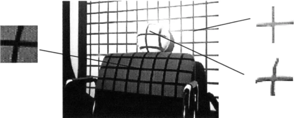
A sample grid image is shown in the following figure uses a ball and a chair as the scanned objects. We as humans can easily follow the grid lines from top to bottom or from left to right. However, a computer looking at this picture faces many difficulties. Our original approach to the problem of extracting intersection was to "trace" the grid lines, hoping to find the intersections from the traces. We attempted to find the start of the grid line along the top edge of the image, then scan the three pixels right below and choose the darkest pixel to be the next point in our growing "line" trace. However, this approach suffered many serious drawbacks and often failed in the following cases:

" Shadows: The algorithm could not tell that it should terminate when it runs into

shadow, which are large patches of black where no grid lines can be seen.

* Varying Brightness: The color of the grid lines could vary between pitch black and very light gray due to uneven lighting, which often resulted in micro "breaks" in the grid lines. Although people can easily tell how the line continues, the algorithm could not.

* Varying Contrasts: The contrast between the grid line and the background on which it was cast could vary greatly due to uneven lighting and the color of the scanned

subject.

* Grid Intersections: When tracing a vertical line downwards, the algorithm had problems at grid intersections, because following the darkest pixel often led it to follow the horizontal line instead.

Varying Contrast Grid Intersections Varying Brightness Shadow

Figure 4. Difficulties of tracing grid lines. These problems forced us to abandon the "tracing approach" to finding grid intersections.

Many "special case" solutions were added to the algorithm in an attempt to solve the problems outlined above. If this algorithm had worked, we would need to take just one single picture of the scanned subject - which would mean that we could decrease the cost of the system even further by using a simple overhead projector. But in the end we felt that this "tracing" algorithm was simply not workable, and were forced to abandon it in search of a better design.

4.2.2 The Solution

In Section 3.6 "Design Overview: Processing" we have already seen a high level tour of the final processing solution. Instead of recapping the processing steps here, we will just highlight the two major differences from our original "line tracing" concept:

* Base Image: We take an additional picture call the base image, which is picture of the subject without the grid line projected over it. Instead of trying to trace the grid lines from the grid image (where the grid is projected over the subject), we will subtract the grid image from the base image. The resultant image contains only the difference of the two - the grid lines.

* Pixel Filter: Instead of tracing the lines to find the grid intersection, pixel filtering is a radically different approach that looks for grid intersections by picking the pixels that matches a certain pattern.

This solution proves to be much more elegant and reliable than the "trace" approach. By subtracting the grid image from the base image, we no longer have problems with shadows, because it is present in both images and are removed. We no longer have problems with varying contrasts, since the background and the scanned subject are not present in the result image. By using a pixel filter to identify the grid intersections, we no longer need to worry about "tracing" the lines correctly. The next section will be devoted to the working of the pixel filter.

4.3 PIXEL FILTER 4.3.1 Introduction

The pixel filter alters the color of an image by examining the color of each pixel and transforming its color using the filter function.

F(x) = x' where F is the filter function, x is the color of the pixel, and x' is the new color of the pixel

The simplest example would be the "identity" function, where x = x' (input color is the same as the output color) and the image is not modified. Another example could be the "map-black-to-white" function, which says:

IF x = black THEN

x'= white

ELSE x'= x

This function turns all the black pixels in the image into white ones, while leaving all other colors unchanged. Pixel filter could be arbitrarily complex. The filter function could take many arguments and calculate the transformation based on multiple input values.

Figure 5. Demonstration of a simple "map-black-to-white" pixel filter. The original picture is on the

left. The filtered picture is on the right, whose windows have been filtered to the color white. 4.3.2 Grid Intersection Filter

In our 3-D scanning image processing, we can use pixel filter to find out where the grid intersections are. Looking at the grid intersections, we notice that all intersection points share roughly the same pattern. As illustrated in the following figure, the three different grid

Figure 6. Close-ups of grid intersections show that they share a highly similar "cross" pattern.

intersections look like they have very different curvatures in the picture, but when we enlarge the intersections by themselves, they share a highly similar "cross" pattern.

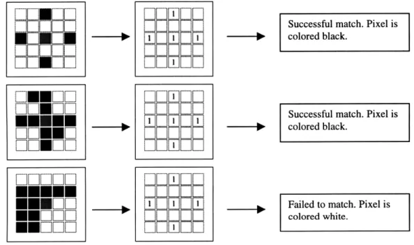
To capture the intersection points, we created a 5-pixel by 5-pixel template to describe this "cross " pattern, and then constructed a filter to find pixels whose surrounding region matches the template. The pixels that match the pattern will remain black; otherwise they will be colored white. The matching template works as follows:

" The middle cell of the matrix corresponds to the pixel being transformed / filtered. * Each cell in the matrix may contain a value that describes the weight of that pixel. If

the cell has no value, then that pixel is completely ignored.

* If the pixel's surrounding region matches the template, then its color is unchanged. Otherwise, the pixel gets filtered out. In our case, the pixel is colored white.

Successful match. Pixel is

1 colored black.

ZiEL

DENFIDIC

OnNFIF-e3ENNET~

Successful match. Pixel is

-1 colored black.

F*r iFI

1

colored white.

I I

Figure 7. Pattern matching with pixel filter. Here we

demonstrate three scenarios and the filter results.

The above figure illustrates how our pixel filter works. We see three sample pixels being filtered (highlighted in red). We need to decide whether these pixels should be colored black or white. The left column shows the colors of the 25 pixels surrounding the pixels in

question. We match the 25 pixels against our template (shown in middle column). A match is successful only if for all the value "1" cells in the template, the corresponding pixel has the color black. If the template cell has no value, the corresponding pixel is ignored.

4.3.3 Implementation

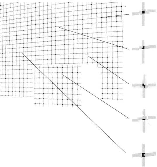
We have implemented this pixel filter in Java, and the algorithm works remarkably well. The following picture shows the filtered image (with filtered grid intersections points in red) layered over the original grid line picture. The pixel filter has highlighted all the intersection points. .4' ' 4 4 . - . .4 a: 4 ' 4" 4 4i '4 'i'** 4~~ .'

.

Figure 8. Result of pixel filter and sample enlargements to show details at grid intersections. The pixels selected by the filter are highlighted in red.

In the figure above, notice in the enlargements that usually the filter selects a cluster of 2 to 5 pixels for each intersection. In our prototype implementation, the program processes these clusters further and selects one pixel from each cluster. We will discuss the details in Chapter 6. The complete listing of the program is available in the appendix.

1 ..

4.4 IDENTIFY INTERSECTIONS 4.4.1 The Problem

In the previous section we saw that we can use pixel filter to extract the intersection points from our images. However, these intersection points extracted are meaningless by

themselves. We need to be able to map all intersection points in the grid image at (x', y) to their original locations in the reference image at (x, y). Then, we can calculate the

displacement of each intersection: (x'-x, y'-y), and complete the quantification of grid distortion.

We call this mapping problem the "identification of intersections". This problem is difficult because the scanned subject's three-dimensional physical volume and its shadow obstruct some grid lines from the camera's view, so we do not have a straightforward 1-to-1 mapping from the grid image to the reference image. Furthermore, from the grid image alone, we cannot determine which grid lines are obstructed or how the grid lines have shifted compared to the reference image. Why? Because all the grid lines look identical to each

other.

In the rest of this section, we will describe our first two failed attempts at solving this problem, and then we will present our final solution.

4.4.2 Two Failed Attempts

Attempt #1: Grid Line Tracing. Originally, we had hoped to be able to trace the grid lines and be able to tell how the line shifts when it hits the scanned subject. If we could follow all the lines correctly, we could reconstruct the grid and determine where the intersections from the reference image have move to in the grid image. Unfortunately, this approach failed for the following reasons:

* Difficulties with Grid Line Tracing: As we have outlined in section 4.2.1, writing software to trace lines in a picture is ridden with difficulties. We were not able to solve these problems.

* Grid Line Shifts Arbitrarily at the Border: When the vertical grid line falls on the subject, it "breaks" at the border and shifts horizontally. It is impossible to tell how much the line has shifted by examining the grid image alone, as illustrated in the following figure.

Figure 9. The problem caused by breaks and shifts of grid lines: In the pictures above, we try to reconstruct the grid line in two different ways, but it is impossible to tell which one is correct from the images alone. The one on the right is actually correct, demonstrating that

grid lines can shift significantly when they land on the scanned subject. Attempt #2: Colored Grid Lines. We also considered marking the grid lines with

alternating colors (for example, red, green, blue, and yellow) so that when the line breaks and shifts we could identify the lines by its color. Unfortunately this approach was not a

workable solution either for the following reasons:

* The Projected Color is Imperfect: When the project casts a black line onto the white back plane, the line looks consistently black to the human eye. However, when the digital camera captures the image, we see that the "black" line actually has various hints of blue, green, and even yellow. We believe that the uneven projected lighting at different parts of the image causes the camera to capture different colors for the "black" line.

* Change in Background Color Changes the Line Color: Even with the imperfection of the projected color, we could still tell the colors apart pretty well when the lines are projected on a white background. However, the line colors are affected dramatically when the lines are projected onto the scanned subject, which could have all kinds of different colors. The blending of line colors and background colors made it very difficult to identify lines based on their original colors.

4.4.3 The Solution

After the two failed attempts, we decided to take another picture so that we could collect more information to help us map the intersection points from the grid image to reference image. We call this the synchronization image.

The synchronization image has a number of squares positioned roughly to cover the size of

the subject. We project this image on to the scanned subject and record where the five

squares are located. Since the positions of these squares are predetermined, we know where

they should be in the reference image, and we can use them to map intersection points in the

grid image to their original locations in the reference image.

Point A

Point A

Figure 10. Identify Intersections: By following the black squares, we can tell where point A in the reference image (top) have move to in the grid image (bottom)

The figure above illustrates this procedure: In the reference image on top (where the grid is not distorted), we know that intersection point A is located at the top right comer of the synchronizing square. Now, how do we find point A in the grid image? We first find the location of the synchronizing square, then we know that point A is the point located at the top right comer of the square. Once we know point A, all other points can be identified relative to A. We will be discussing the details of implementing this procedure in Chapter 6.

5

CONVERTING DISTORTIONS TO DEPTHS

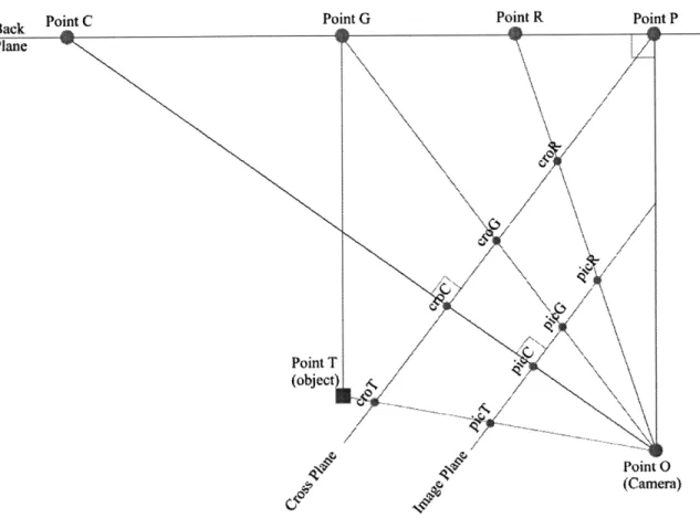
In this section, we will present the optical model used to convert horizontal distortions to depth information. The mathematics is fairly straightforward trigonometry. The greatest difficulty was in constructing the actual model and verifying its correctness. The following figure is a graphical summary of the model. We will be explaining the setup, the

assumptions, the requirements, and the calculations.

Point C Point G

Point T

Ao Ak- Point O

o ,(Camera)

5.1.1

Setup

The optic diagram models the view of the camera (point O) when it is capturing an image of

the back plane. The projector (not shown in figure) casts a grid onto the back plane. We

choose a single vertical grid line, which is point G in the diagram. When we place a subject

in front of the plane, our chosen grid line lands on the subject (point T).

Then, we choose another grid line that lands on the back plane as point R. This point serves

as a reference point so that we can calculate the ratio between real distances and pixel

distances. Point R can be any grid line as long as it is within the view of the camera.

Next, we fixe the camera so that the center of its view corresponds to point C on the back

plane. When the camera captures an image, the particular view can be represented as a line

(picture line) that is perpendicular to the line-of-sight from the camera to point C.

Now we can locate the perpendicular point P on the back plane. Line PO is the shortest

distance between the camera and the back plane. We extend another imaginary line from

point P (cross line) which is perpendicular to line

CO.

This line is needed to complete the

trigonometry calculations. Note that point P does not need to be in the view of the camera.

5.1.2

Given

From the images, we will have the distortion of grid lines in terms of pixel distances. In the

figure, this is the distance croGcroT. (Chapter 4 details the quantification of grid line

distortion). We are also given the pixel distance between point R and point C (in the figure

this is the line picRpicC). This is a one-time measurement needed to find the ratio between

real and pixel distances.

5.1.3

Objective

We want to calculate the length of GT, which is the distance between the object and the

back plane (i.e. the depth of the subject at that point).

5.1.4

Measurements

The following distances are required to bootstrap the calibrations and calculations.

Length of PO: The shortest distance between the camera (point 0) and the back

plane, which is the perpendicular point P.

* Length of PR: The distance between the perpendicular point P and the reference point R.

* Length of PC: The distance between point P and point C, which is the center point in the camera's view.

* Width of grid: The horizontal distance between two adjacent vertical grid lines. 5.1.5 Calibrations

The four measurements alone would have given us the parameters necessary to complete the model - if the projector were not a point source of light. Unfortunately, the point source nature of the project means that light travels away from the project at an angle (ZRGT), which must be measured to ensure the accuracy of the model. However, hand-measuring this angle for every grid line is a very time-consuming and error prone process. Therefore a calibration run is needed to calculate ZRGT for each grid line.

5.1.6 Calculations

Once we have taken the measurements and calibrated the angles, we can calculate our objective, distance GT.

First, we find the real distance to picture ratio.

ZPCO = arctan PO

RcroC = CR - sin(ZPCO) RcroC

ratio = RoC picRpicC

Using the ratio, we can begin to calculate all the other distances and angles in the model. We start with finding ZTOC.

croTcroC = (picRpicC - picRpicT) - ratio

:-2 -2

croCO =RO -RcroC

ZTOC

=

arctancroTcroC

Then, we find ZPGO and ZROC. GP = CP - CR + GR ZPGO = arctan PO GP ZPOG = - ZPGO 2 ZROC = - - ZPCO 2

Now we can completely characterize the triangle OGT.

ZGOT = ZROC - ZPOG - ZTOC

ZGTO = 7r -ZOGT -ZGOT

GO= GP +PO ZOGT = ZRGT - ZPGO

Finally, we will use the sine rule to find GT.

GT = GO- sin(ZGOT)

sin(ZGTO)

5.2 MODEL VERIFICATION

We have verified the model using a simple test setup. In this experiment, we setup the camera and projector and took the four required measurements.

PO = 815.98mm PC = 488.00mm PR = 205.00mm

GridWidth = 30.71mm

Next, we calibrated seven grid lines by calculating their ZRGT angle. We took images of an object of known and uniform depth and then calculated the angles. The next table

GR (mm) 61.43 92.14 122.86 153.57 184.29 215.00 245.71

picRpicT (pixel) 124 151 176 201 224 247 269

ZRGT (degrees) 95.23 94.95 94.32 94.11 93.48 93.24 92.96 GT (depth of rectangular box)= 177mm

Table 1: Summary data from test calibration Then, we placed a cylindrical

object and calculated its depths along the surface based on the ZRGT from our calibration run. We also hand measured

the depth of the cylinder at

those points so that we could compare the magnitude of

error.

Figure 12. An image of our test setup. The cylindrical object was our scan subject. The white box below (with

known and uniform depth) was used for calibration. ZRGT (degrees) 95.23 94.95 94.32 94.11 93.48 93.24 92.96

picRpicT (pixel) 124 167 207 240 267 290 308

GT(mm) 177.00 207.41 231.51 245.00 250.67 249.43 242.26 Real depths (mm) 177.00 208.00 232.00 245.00 250.00 249.00 242.00

Error 0.00% -0.28% -0.21% -0.00% 0.27% 0.17% 0.11%

Table 2: Summary data from scanning a cylindrical object.

We were pleased to find that the error margins to be ±0.30%. This simple experiment confirms that our optic model is correct (other earlier but incorrect versions of the model had errors on the order of 30%!) However, having the correct model, we still have to deal with certain calibration and hardware inaccuracies:

* Measurement from Center of Camera: Our measurement requires that we take the shortest distance from the camera to the back plane. However, the center of the camera lens is difficult to pinpoint, as the lens is encased in plastic shell.

* Camera Resolution: When extracting grid intersection from the images, we are limited to the resolution that the camera can provide. Having a higher resolution would let

us calculate grid distortions with higher precision, and thereby increasing the accuracy of the depth data.

Other Camera and Projector Distortions: The spherical nature of the camera lens can cause distortion in the image. This problem is especially significant at the outer border of the image: instead of capturing straight grid lines, we could have lines that seem bowed. The projector can also contribute to this problem. Much like the way a monitor could cause distortion of image on the screen, the projector can adjust pincushion, trapezoid, and

orthogonality properties. A faulty or incorrectly adjusted projector could cast a distorted grid.

Figure 13. Camera and projector distortion. In the image above, the vertical lines on the left are parallel to the vertical edge of the image, but the vertical lines on the right are seriously slanted.

Can these problems be solved? The answer isn't clear. Fundamental hardware problems can be fixed by using better hardware, but finding software approaches to compensate for hardware inadequacies can be very difficult. Overall, we believe that our model is correct, as we were able to achieve the ±0.3% error margin.

6

IMPLEMENTATION OVERVIEW

6.1

For the purpose of demonstration, we have implemented the algorithms in Chapter 4 and the optical model in Chapter 5 to produce a prototype scanner. In this chapter, we will first give an overview of the setup and functionality of the prototype unit. Then we will focus on

the details of each of the functional components in Chapter 7.

For our prototype setup, we used a Polaroid Polaview 201 projector to cast the grid and a Polaroid PDC-2000 digital camera to capture the images. Both the camera and the projector operated at resolution of 800x600 pixels. The processing application was implemented in about 2,500 lines of Java code and ran on a Pentium 166MHz PC running Windows 95 with 32 MB of memory. The wall served as the geometric back plane and was assumed to be perpendicular to the floor.

To get our prototype up and running, we first took the required measurements to setup the optical model.

* PO Shortest distance from camera to point P on the back plane

" PC Distance from point P to point C, center of camera's view * PR Distance from point P to point R, reference point.

* Grid width Horizontal distance between two adjacent vertical grid lines

Then we took the following reference images. Notes that Wall denotes the back plane, Grid denotes the grid lines, and Sync denotes the synchronization square. Wall + Grid means that the image is taken with the grid projected onto the wall.

* Wall

* Wall + Grid * Wall + Sync

Next, we placed the calibration object and took three more images. * Wall + Object

* Wall + Grid + Object

We then fed all the data and images to our processing application for a calibration run. The

program produces a calibration data file.

Once we have completed calibration, we can now take images of other objects and feed

them into the applications. The program will produce a 3-D model file containing (x, y, z)

points of the object. This 3-D model file can then be imported into a variety of graphics

programs for viewing.

6.2

PROCESS FLOW

Our processing application processes the six images following the sequential order of steps

below to either produce the calibration angle data or the (x, y, z) depth points of the scanned

object:

" Process Reference Images

* Process Object Images

* Synchronization Mapping

* Run Optical Model

In the rest of this section, we will discuss these four steps individually and see how we can

go from 2-D images to 3-D data points. For clarity, we will be explaining the intermediate

steps an "input -

procedure

output" notation. In this chapter, we will treat the

"procedures" as black boxes with the specified functionality. In Chapter 7, we will look

inside these black boxes and discuss how they are actually implemented.

6.2.1

Process Reference Images

The reference images are the ones taken without the scanned object. We need two pieces of

data from these images:

* RefIntersectPts: Array of intersection points location (x, y).

* Ref_Sync_Pt: Location of the synchronization point.

The processing consists of four intermediate steps:

(Image of Wall+Grid, Image of Wall) I Image Subtractor ~- (Image of Reference Grid)

(Image of Reference Grid) -I Intersection Extractor (RefIntersectPts)

(Image of Reference Sync) -4 1Sync Extractor (Ref_SyncPt)

We will briefly describe the functionality of the black box procedures mentioned above: Image subtractor takes two input images and returns a new image that contains the difference

of the two. Intersection extractor takes a grid image and returns an array of intersection points at (x, y). Sync extractor takes a sync image and returns the location of the synchronization square found in the image. We will discuss their implementation details in the next chapter. In practice, the processing of reference image only needs to be done once for every

calibration. However, in our prototype implementation we have included the processing in every run for demonstration purposes.

6.2.2 Process Object Images

The object images are the ones taken with the scanned object. We need two pieces of data from these images:

* Obj_Intersect_Pts: Array of (x, y) which are locations of intersection points covering the scanned object.

* Obj_SyncPt: Location of the synchronization point.

The processing consists of six intermediate steps that give us the two items that we need:

(Image of Wall+Grid+Obj, Image of Wall+Obj) -+ Image Subtractor l (Image of Object Grid) (Image of Wall+Obj, Image of Wall) - Image Subtractor (Image of Object Outline)

(Image of Object Grid, Image of Object Outline) - Image Subtractor (Image of Obj Outline Grid) (Image of Object Outline Grid) - I Intersection Extractor - (Obj_Intersect_Pts)

(Image of Wall+Obj+Sync, Image of Wall+Obj) - Image Subtractor -- (Image of Object Sync) (Image of Object Sync) I Sync Extractor (Obj_Sync_Pt)

Notice that we have added a step to find the outline of the object. The object outline helps us eliminate the intersection points that are not on the object, and therefore reduces the processing work significantly.

6.2.3 Synchronization Mapping

Now that we have processed the images and collected the intersection points into arrays, we are ready to synchronize the object image with the reference image. With the help of the

synchronization points, we will map all the points in the object image to their original

location in the reference image. We produce the MappedArray, whose elements are the

coordinates (Obj_x, Obj_y, Ref_x, Ref_y).

(RefIntersectPts, RefSync_Pt, Obj_Intersect_Pts, Obj_Sync_Pt) -- Point Mapper -4 (Mapped_Array)

6.2.4 Run Optical Model

We have now completed the entire image processing work. The Mapped_Array tells us quantitatively how the intersection point have moved from their original location in the reference image to their 'distorted' location in the object image. Having this data, we can finally run the optical model. There are two different ways to use the optical model., depending on whether this is a "calibration" run or an actual "scan" run.

First, we can use the model to calculate the RGT angles for calibration. Recall from Chapter 5 that these angles are formed by the light rays traveling from the projector to the back plane, and that for every vertical grid line, we need to calculate its RGT angle. For calibration, the object being scanned must be of known and uniform depth and we must provide the pre-measured depth of the object. The program will give us a calibration data

file containing the angle data for each of the vertical grid lines.

Calculate angles: (Mapped_Array, Real_ObjectDepth) -- Optical Model - (RefxData) (Ref xData) -- File Writer - Calibration Data File

Once we have the calibration data in place, we can give the program images of arbitrary objects, and the program will give us a 3D Model File containing the (x, y, z) data points of the object.

Calculate depths: Calibration Data File --4 File Reader -- (RefxData)

(Mapped_Array, Ref x Data) -- Optical Model (real_x, real_y, z)

(real_x, real_y, z) - I File Writer ---> 3D Model File

We have finally produced a 3-D data file from the 2-D images! In the next chapter, we will discuss the implementation of the black-box procedures used in all the intermediate steps in detail.

7

DETAILS OF PROCESSING COMPONENTS

In the previous section, we explained the processing flow with a handful of procedures which we treated as "black boxes". In this section, we will look inside these black boxes and see how they are actually implemented. The three we will examine are: image subtractor, intersection extractor, and point mapper. The optic model component is not explained here because we have already detail the optic mathematics in chapter 5.

7.1 IMAGE SUBTRACTOR

The functionality of the imager subtractor is very simple: take two input images, subtract the color on a pixel by pixel basis, and return the resultant difference. In our implementation, we go one step further and turn the images from "red, green, and blue" colors into black and white. This is to facilitate processing by other components that will use the image as their inputs.

We ended up with a simple implementation of the image subtractor because the input

images from our prototype setup subtract very cleanly. If the input images are noisy or if the camera performs any kind of automatic image adjust, this component will need to be

extended to handle the additional processing.

7.2 INTERSECTION EXTRACTOR

The goal of the Intersection Extractor is to take the image of the grid lines, and produce an

array of (x, y) points that are the grid line intersections. Chapter 4.2 gave detailed description

of this problem and the design of the solution. Here, we will focus on the implementation

of the solution.

The task of extracting intersections can be broken into two smaller steps:

Step 1: {Image of grid lines} -

I Pattern Filter -- {Image of intersection points}

Step 2: {Image of intersection points}--+ Grid Point Processor --+ {Array of (x, y) points}

We will now describe the two components, Pattern Filter and Grid Points Processor, that

help us extract intersection points.

7.2.1 Pattern Filter

The pattern filter component takes a grayscale image of the grid lines, and outputs an image

of grid line intersection points. Recall from Chapter 4.3 that filtering works on a pixel by

pixel basis, assigning a new color to each pixel based on how well its surrounding pixels

match a given pattern.

Pattern description file: In our prototype implementation, we let the user describe the

desired pattern in an external file. Below is the pattern file used in our prototype to filter out

the grid intersection points. The first five lines specify parameters about the pattern,

followed by the coefficient data for the actual pattern itself:

10101

00000

00100

"Row" and "col" specify the dimension of the pattern. "Targetrow" and "targetcol" specify

the location of the pixel to be filtered in the pattern. "Threshold" specifies the upper bound

for the color of a "matching" pixel, ranges from 0 (black) to 255 (white).

Filtering process: The pixel to be filtered is called the target pixel. The pattern is matched

against the area of the same dimension surrounding the target pixels. Wherever the

coefficient is '1' in the pattern, the corresponding pixel must have a color value that is less

than the threshold value. If all the pixels marked with '1' in the pattern have color value less

than the threshold, then the target pixel is colored black. Otherwise, the target pixel is

colored white. For a more graphical explanation, please see Chapter 4.3.

Image boundary: The filtering process is very

straightforward, but it does have its tricky

boundary cases. As we move our pattern

template across the image a pixel at a time, we

will have problems with our calculations

whenever we come to the borders of the image.

As shown in the picture on the right, this

problem is caused by the pattern "hanging over"

I I

Figure 14. Pixel filter "over hanging" at the edges of the image. We need to take special care of these boundary conditions.

I 1

Patter hangi the in

the edge of the input image and there are no pixels to match the pattern. This problem occurs at the top, left, right, and bottom borders of the image. We considered some different methods to cope with this problem:

* Completely ignore the data at the edges of the image and do not filter those problematic pixels.

" Replicate data at the edges of the image, or give the missing data a default "fill-in"

value. Then perform filtering as usual.

In our implementation, we decided to completely ignore the data at the edges of the image. Our choice means that we lose all that data at the edges of the image and that the scanned subject cannot be placed at the edges. However, since the edges often contain noisy or distorted data, we feel that it is advantageous to lose the edges anyway.

These components are implemented in the classes PatternFilter, PatternParser, and

Pattern. For code listing please see appendix. 7.2.2 Cluster Processor

The pattern filter gives us an image of the intersection points. To know exactly where these intersection points are, all we have to do is pick them off the image and record their (x, y) locations. How difficult can this be?

Indeed, the problem seems easy at the first sight. The pattern filter does give us a clean image of the

intersection points. But when we zoom in and examine the image at the pixel level, we see for every intersection, the filter gives a cluster of pixels, as shown in the figure on the right. This is because the grid lines are more than one pixel thick, and the "clusters" in the image reflect the thickness of the grid lines.

E

%

N

Figure 15. Close-ups of the image

show that the pixel filter gives irregularly shaped clusters of pixels.

These "clusters" poses significant problems for several reasons:

For every grid intersection, we only want one pixel representing that intersection. This means that for every cluster, we must choose a pixel from it, using a consistent heuristic. In our prototype, we choose the lower-rightmost pixel from every cluster.

* To make a consistent pixel choice, we need to locate the cluster in its entirety so that we can find, say, its lower-rightmost pixel. However, these cluster come in

completely unpredictable shapes, so profiling them is difficult.

* To make things even more complicated, the locations of these clusters are not predictable or known, so we need an algorithm can locate clusters in arbitrary locations.

Cluster locating algorithm: Fortunately, we have found an algorithm that can locate clusters reliably and quickly. Scan across the image from top to bottom, starting at the

upper-left hand corner and sweeping to the right. To keep track of which pixels have been examined, we attached a "visited" flag to all the pixels we have processed. The description of the algorithm is organized into the following pseudo code format for clarity:

Loop over the entire image. For every pixel at x, y:

{

If (pixel color = white)

Then pixel does not belong to a cluster. So skip to the next pixel. If (pixel color = black && pixel is marked "visited")

Then pixel already belongs to a cluster that we have processed. So skip to the next pixel.

If (pixel color = black && pixel is not marked "visited")

Then pixel is part of a new cluster. Call ProcessCluster (x, y) Mark the pixel as "visited"

Finding cluster's bounding box: The ProcessCluster function locates the entire cluster by

incrementally exploring its neighboring pixels. Since we are scanning the image from top to bottom, we know that the new pixel we just found must be in the top row of the cluster. Therefore we only need to look in three directions (left, right, and below) until all the neighboring pixels are white. In our implementation, we keep track of the bounding box of the cluster, and we expand incrementally expand the box to enclose the entire cluster. ProcessCluster (x, y)

{

//InitiaHze bounding box variables

box_x_left = box_x_right = x

box_y_bottom

=

box_y_top

=

y

saw_more_black_pixel = true

// Loop as long as we are stillfinding black pixels While (saw_more_black_pixel = true) {