HAL Id: hal-02307900
https://hal.archives-ouvertes.fr/hal-02307900
Submitted on 8 Oct 2019
HAL is a multi-disciplinary open access
archive for the deposit and dissemination of
sci-entific research documents, whether they are
pub-lished or not. The documents may come from
teaching and research institutions in France or
abroad, or from public or private research centers.
L’archive ouverte pluridisciplinaire HAL, est
destinée au dépôt et à la diffusion de documents
scientifiques de niveau recherche, publiés ou non,
émanant des établissements d’enseignement et de
recherche français ou étrangers, des laboratoires
publics ou privés.
biplane angiographic sequences using parametrically
deformable models
Laurent Sarry, Jean-Yves Boire
To cite this version:
Laurent Sarry, Jean-Yves Boire. Three-dimensional tracking of coronary arteries from biplane
angio-graphic sequences using parametrically deformable models. IEEE Transactions on Medical Imaging,
Institute of Electrical and Electronics Engineers, 2001, 20 (12), pp.1341-1351. �10.1109/42.974929�.
�hal-02307900�
Abstract-- A new method for coronary artery tracking in biplane digital subtraction is presented. The dynamic tracking of non-rigid objects from two views is achieved using a generalization of Parametrically Deformable Models. 3D Fourier descriptors used for shape representation are obtained from the 2D descriptors of the projections. A new constraint inferred from epipolar geometry is applied to the contour model. Direct 3D tracking is compared to the classical approach in two steps: independent 2D tracking in each of the two projection planes and 3D reconstruction using the epipolar constraint. Convergence quality and accuracy of the 3D reconstruction are analyzed for several sequences showing different displacement amplitudes, deformation rates and image contrasts.
Index Terms--– 3D reconstruction, biplane angiography, deformable contour model, dynamic tracking.
I. INTRODUCTION
HE recovery of 3D object features is an important application of stereoscopic vision. New developments involve the temporal dimension to enable motion estimation. Digital subtraction angiography provides imaging sequences on two different views. Subtraction itself is rarely applied for coronary arteries in interventional cardiology due to permanent movement of the heart and surrounding tissues. But non subtracted acquisitions may be used to track coronary arteries with more or less user interaction to obtain morphological and dynamic description of vascular trees [1]-[5]. They can be used in several ways: motion analysis [6], [7], optimal viewpoint determination [8]-[10] or as automatic delineation for the measurement of 3D densitometric content. Indeed, several works showed that spatiotemporal density variations inside the artery bed provide functional information like absolute blood flow velocity, and consequently stenosis ratio and coronary flow reserve [11]-[15]. Biplane angiography is for now the only imaging system that enables to record a short-live contrast medium bolus at a high acquisition rate, while allowing to access to 3D geometry of the vessel centerline. Multi-slice CT [16], rotational angiography [17] and MRI techniques [18] are better designed to assess the full 3D geometry of a coronary artery tree than to perform vessel tracking, because one acquisition at a given time of the cardiac cycle requires ECG gating to overcome motion artifacts. In the case of biplane angiography, computerized tomography
L. Sarry and J.-Y. Boire are with the Medical Image Research Team (ERIM), Faculty of Medicine, Auvergne University, BP 38, 63001 Clermont-Ferrand, France (email: [email protected]).
techniques are unusable with only two views and when opacification is no longer stationary. Therefore, a computer vision approach is proposed in this paper, involving a new 3D contour model based on Fourier shape descriptors and epipolar constraint for non-rigid object tracking in order to minimize user interaction. This principle was already experimented for intravascular ultrasound (IVUS) catheter segmentation using a B-spline parameterization [19].
In 3D contour tracking processes, two stages are usual: 2D dynamic tracking in both projection planes (segment matching): the new 2D centerline is inferred from last location and intra and/or inter frame information. In a previous paper [20], we proposed a comparison of several deformable models to perform the first step. Classical Active Contour Models [21] are unable to track vessels reliably between two consecutive images when movement is greater than vessel radius. Results are somewhat improved by the use of velocity field estimation [22], [23], but constraints based on optical flow calculation are not valid in case of strong deformation as well. Instead of describing a contour with its exhaustive set of points, we used a limited set of shape descriptors. A deformable model, called the Parametrically Deformable Model, was first designed in [24]. We have successfully implemented it for coronary artery tracking. Robustness is increased by the fact that each point is implicated in global shape behavior and that pattern deformation is limited in spatial extent leading to a shape memory effect.
* 3D reconstruction of vessel centerline (point matching). For methods based on motion detection, the estimated velocity field is used to pair points between the two projection views [3], [4], while other methods use constraints inferred from the epipolar geometry of the biplane system [25].
In the first part of this paper (paragraph II-A), the principle of 2D and 3D shape descriptions are introduced. Paragraph II-B concerns the geometric attributes of the biplane system. In paragraph II-C, the 2D method in two distinct steps is described. The principle of Parametrically Deformable Models in two dimensions is presented. The point matching problem is considered from a different angle in that it does not require any reference point on the projected contours. This paper concerns the application of Parametrically Deformable Models to the real 3D dynamic tracking of a coronary artery. In paragraph II-D, the deformable model is generalized to take into account the image information in both planes and the epipolar constraint. Advantages of the new description concern convergence robustness and 3D reconstruction precision thanks to a strong immunity towards image parasitic content
Three-Dimensional Tracking of Coronary
Arteries from Biplane Angiographic Sequences
using Parametrically Deformable Models
Laurent Sarry and Jean-Yves Boire
(noise, overlapping objects) and stereoscopic calibration inaccuracies.
II. METHODS
A. Shape description
The basic problem is to recover the 3D centerline of one artery segment during a whole angiographic sequence. Biplane digital angiography provides temporal sequences for two different incidences, thus it gives access to the 3D dynamic geometry, but it suffers from an intrinsic technical limitation: images on planes A and B are acquired in an interlaced way (Fig. 1). At time t of the acquisition on plane A (resp. B), the vessel projection At (resp. Bt) is determined, but the
corresponding contour on the other plane Bt-1|t (resp. At|t+1) is
unknown. Instead of time interpolating the missing images prior to reconstruction as in [26], the shape descriptors are approximated using linear interpolation as follows:
1
2 1 t t t t A A A and Bt1t
Bt1Bt
2. (1)Interpolation of shape descriptors is equivalent to interpolating contour points because of the linearity of discrete Fourier transform. Figure 2 gives a schematic overview of one 3D contour, its corresponding projection on the existing image plane and the interpolated projection on the other image plane. The 3D contour corresponding to a vessel feature can be described by an exhaustive set of points, equally sampled along the length L. Each point location is uniquely determined by its arc length s along the contour:
xs y s z s s L
C ( ), ( ), ( );0 . (2)
Parametric representation affords the same shape information with only 3(N+1) parameters:
N i N i N i L s s z s y s x C 0 ; p = 0 ; p = 0 ; p = 0 ; ) ( ), ( ), ( i z i y i x z y x p p p p p p z y x (3)The choice of Fourier shape descriptors [27] eases the calculation of the parameter vectors px, py and pz. Coordinate functions x(s), y(s) and z(s) are expanded into Fourier series by means of discrete Fourier transform F (FFT algorithm). Only a few Fourier coefficients pi are needed because vessel
shapes are smooth (N ranging from 10 to 20). The computation of the Fourier descriptors for an open shape requires double sampling of the contour in the following manner:
points 1 to M are the M sampled points numbered along the direction of blood flow,
points M+1 to 2M are the same points numbered in the reverse direction.
The resulting function of coordinates versus arc length is symmetric relative to the coordinate s=L. Fourier coefficients are no longer complex numbers, but real quantities:
N k z y x z y x L ks k p k p k p p p p s z s y s x 1 cos ) ( ) ( ) ( ) 0 ( ) 0 ( ) 0 ( ) ( ) ( ) ( . (4)For the 2D projected contours, the same description has 2(N+1) parameters with vectors pu and pv for u and v
coordinates. The contour coordinates are obtained from the Fourier descriptors by reverse discrete Fourier transform F-1. Zero padding is used to fill in the descriptor vector from N to L harmonics.
B. Biplane system description
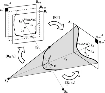
The biplane system is characterized by three different spaces for shape representation: two spaces of dimension 2 in each of the image planes and one space of dimension 3 corresponding to the world coordinate system. Two different reference coordinates may be used to locate a point in space: coordinates related to image plane A and coordinates related to image plane B. B PLANE SPACE A PLANE ) , ( ) , , ( ) , , ( ) , ( B A (R,t) M M A A A B B B B B A A v x y z x y z u v u
Let (iA, jA) and (iA, jA, kA) be the respective 2D and 3D reference coordinates of projection view A, where iA, jA, kA are orthogonal to each other. Let (iB, jB) and (iB, jB, kB) be the respective 2D and 3D reference coordinates of projection view B, where iB, jB, kB are orthogonal to each other. The transformation (R,t) is the 3D displacement (rotation matrix R and translation vector t) from a point mAT = (xA, yA, zA) in the
plane A coordinate system to a point mBT = (xB, yB, zB) in the
plane B coordinate system. The homogeneous coordinates M~ of a given 3D point M in the world coordinate system and its homogeneous retinal coordinates m~A and m~B are related by the perspective projection matrices PA and PB. We assume that 3D coordinates of M are expressed in the coordinate frame of plane A:
and
, with ~ and ~ B B A A B B A A t R M P 0 I M P M P m M P m B A (5) 1 0 0 0 0 and 1 0 0 0 0 0 0 B 0 0 A B B Bv B Bu B A A Av A Au A v u f f v u f f M MA and B are respective arbitrary scales for planes A and B, fA
and fB, are the focal lengths on planes A and B. Au, Av, Bu
and Bv are the horizontal and vertical scale factors, whose
inverses characterize the size of the pixel in the world coordinate system. Finally, (uA0, vA0), (uB0, vB0) are the
coordinates of the principal points, which are the orthogonal intersections of the optical axes with the image planes. For application to optimal viewpoint determination, the orientations of the planes should be relative to the world coordinate system (i, j, k); therefore, [I 0] and [R t] should be replaced in (5) by [RA tA] and [RB tB], the rigid transforms from the world system to the image planes A and B respectively (Fig. 2).
The rotational and translational parameters can be determined from the angulation values provided along with the image data [8], which implies that the isocenter assumption holds. For higher accuracy, they are recovered using the essential matrix estimation from the knowledge of the retinal coordinates of eight or more points [29]-[31]. Such an algebraic method is rather constraining because an offline procedure is required, as well as for the correction of
pincushion distortion which is based on the recording of a rectangular grid and the bicubic interpolation of true coordinates to the whole image plane. This process is to be performed for every calibrated positions of the biplane system, since long-range time drift was proved to be negligible [32]. For higher convenience, correction could be extended to any intermediate position through an interpolation process [33].
C. Two-dimensional tracking on projection views
The 3D vascular structure recovery is performed in two independent steps: a segment matching problem and a point matching problem. The first step is solved by independently tracking 2D vessel projections in both planes. Contours on planes At and Bt are determined on the whole angiographic
sequence. Contours At and Bt-1|t, and contours At|t+1 and Bt
allow us to compute two consecutive vessel locations in space. Then the point matching problem consists in finding corresponding points on both segments. Coordinates of 3D points are inferred from coordinates of the matched points.
1) Segment matching
Fourier descriptors are used to parameterize 2D contours by means of vector pu for decomposition of coordinates u and vector pv for coordinates v. The Parametrically Deformable Model as defined in [24] enables adjustment of the initial shape to the final one on the next image by the optimization of its shape descriptors. Each coefficient of vectors pu and pv is given a Gaussian distribution (means mu, mv and standard deviations u, v), so that the model is constrained to a particular overall shape, while allowing for deformations. Vessel deformation between two consecutive images is considered to be regular. At each step of the optimization problem, the sum of gray levels at the model points described by the parameter vectors pu and pv is calculated to search for intensity valleys. A compromise has to be made between minimization of this sum and preservation of the initial shape. For the image At(x,y), we have to maximize a cost function
with respect to parameters pA = [puT pvT]T:
L A A t nA A v v v v N k u u u u t ds s v s u A k k m k p k k k m k p k A M 0 A A 2 2 2 0 2 2 )) , ( ), , ( ( ) ( 2 )) ( ) ( ( 2 ) ( ln ) ( 2 )) ( ) ( ( 2 ) ( ln ) , ( p p pA (6)A is the maximum gray level of the object of interest in
plane A and nA2 represents the weight between the first term
of shape memory and the second term of image information. It is an equivalent of a signal-to-noise ratio that would characterize the influence of other objects and image noise sources encountered in the vessel search. When many parasitic objects occur in the projection field, we showed that the variance nA2 must be high to encourage the memory effect.
Reciprocally, when the vessel deformation is strong, it must be low to maximize the spatial extent of the object search. Poor results are obtained when low vessel contrast and strong deformation co-occur [20].
2) Point matching
The use of Eq. (1) gives two simultaneous projections of a 3D contour. The geometrical constraint, inferred from the
knowledge of the intrinsic parameters of the two image planes, is used to recover the contour location in the world coordinate system. It is expressed by the fundamental equation, called the epipolar constraint: 0 A 1 A T B T B m TRM M m (7)
E = TR is the essential matrix, and T is antisymmetric matrix such that Tx = t^x, where t is the vector connecting the two x-ray spots of the biplane imaging system, and ^ denotes the operator of cross-product. The matrix defined by MB
-TTRM
A-1 is known as the fundamental matrix of the two image planes A and B. Eq. (7) corresponds to the epipolar line in plane A when the point mB is known in plane B, and reciprocally, to the epipolar line in plane B when the point mA is known in plane A. Points on the two contours are matched using a least-squares criterion defined in [28]. We minimize the sum D of the squared distance of one projection point mA (resp. mB) and the corresponding epipolar line from the other image plane Φ ~mB (resp. Φ ~mA):
L i A B D 1 2 B T 2 B T T A 2 A 2 A T B ~ ~ ~ ~ ~ ~ Φm Φm m Φ m Φ m m (8)The use of dynamic programming to solve this minimization problem has been detailed elsewhere [1], [3].
3) Temporal tracking
At this point, the 3D vessel feature can be reached through segment and point matching steps. To perform temporal tracking, the manual delineation of the vessel centerline is required in both planes for the first image. Then, convergence result of the segment matching is validated or corrected by the user. Two different levels of interaction may be designed: a global correction in case of wrong convergence, which consists in drawing the whole contour again, and a local correction when the model fails for a minority of points. The resulting contour is used as an initialization for the deformable model at the next time step. Then point matching is performed for contours At and Bt-1|t and for contours At|t+1 and Bt.
D. Full three-dimensional tracking
The main drawback of the previous method is that it involves two independent tracking processes and a point to point matching step. The multiplicity of the matching solutions in case of two views induces local minimums in spite of an order constraint along the contour. This section describes a totally 3D one-step tracking that intrinsically includes the vessel reconstruction. It is based on the parametric representation of the 3D contour as described by Eq. (4).
1) Application of the perspective constraint to 3D Fourier descriptors
Because of Eq. (5), the knowledge of one projection of the vessel contour {(u(s),v(s))} induces conditions on the other projection. Indeed, 3D Fourier descriptors are linked by the two following relationships:
withk [0,N] ) )]( ( [ ). ( ) ( ) )]( ( [ ). ( ) ( s k p s v k p s k p s u k p z y z x 1 1 F F F F (9) This equation shows biplane system redundancy. Two out of the three coordinate descriptors (for example px and py) can be calculated from the third one (for example pz) and the 2Dcontour projection. Two interesting properties for numerical calculations stem from the previous formal relationship and the definition of the 3D descriptors (4). The following equations concern results developed in appendix A:
( ) ( )
/2 with k [0,N] ) ( ) ( 2 / ) ( ) ( ) ( ) ( 0 0
N l v v z y N l u u z x k l p k l p l p k p k l p k l p l p k p (10)pu and pv are the vectors of 2D Fourier descriptors previously defined. The harmonics l+k and l-k result from the first 2N coefficients of the Fourier series decomposition of the coordinates u and v. Hence, px and py may be obtained from a single FFT step instead of the two steps stated in (9). The other result concerns the partial derivatives of the descriptor vectors px and py with respect to the descriptor vector pz:
2 / ) ( ) ( ) ( ) ( 2 / ) ( ) ( ) ( ) ( k l p k l p l p k p k l p k l p l p k p v v z y u u z x (11) These derivatives can result from the same previous FFT step. We will see that this expression is useful in the gradient formulation of the objective function.2) 3D Parametrically Deformable Contour model
The new formulation takes into account image gray levels on both projection views and a parameter vector p = [pxT pyT pzT]T. By analogy with the 2D model, the estimation of the 3D contour together with its projection Bt-1|t uses a cost function
M(At, Bt-1|t, p) which is the sum of three different terms:
a shape memory term S(p): the square distance from the coordinate z descriptors pz to the initial ones mz:
N k z z z z k p k m k k S 0 2 2 ) ( 2 )) ( ) ( ( 2 ) ( ln ) (p (12a) a constraint C(At, p) inferred from the known 2D contour
At: given the descriptor vector pz for coordinate z, the associated theoretical vectors px0 and py0 can be calculated using (10). The set of all possible vectors pz defines a skew surface to which 3D contour is supposed to belong when calibration is exact (Fig. 2). To take into account calibration inaccuracies, 3D contour is constrained to stay not into but close to this surface:
2 2
0 0 2 2 0 ) ( 2 )) ( ) ( ( 2 ) ( ln ) ( 2 )) ( ) ( ( 2 ) ( ln ) , ( k k p k p k k k p k p k A C y y y y N k x x x x t
p (12b) and the image gray level information I(Bt-1|t,p) at the
location of Bt in plane B: Bt is calculated from the previous
contour Bt-1 and the projection Bt-1|t of the current 3D contour
using interpolation (1):
L t nB B t t B x s ys zs ds B I 0 2 1 , ) ( (, ), ( , ), ( , )) ( p PB p p p (12c)The same equation can be written for the cost function
M(At|t+1,Bt,p). Numerical solution of this optimization problem
is obtained using the Fletcher-Reeves-Polak-Ribiere version of the conjugate gradient algorithm [34]. The analytical expression of the gradient vector is fully developed in appendix B.
3) Constant length constraint
One of the major drawbacks of open deformable contours of any type is that they have a strong tendency to shrink inside the gray level valleys. It is less acute in case of Parametrically Deformable Models because of the shape preservation term, but it may occur when motion direction is parallel to the vessel orientation. To overcome this limitation, we have used the termination criterion used in case of Active Contour Models [35] as a constraint for our model. This assumption is appropriate since clinical validation for 3D QCA have proved that there was no systematic variability of the length during the cardiac cycle [36]. The constraint consists in bringing the image strength back to one unit of the contour length L(p):
( (, ), ( , ), ( , ))
( ) ) , ( 0 2 1 p B PB x sp ys p z s p ds Lp B I L t nB B t t L
(13)The calculation of the contour length from the descriptor vector p is developed in appendix C.
4) Temporal tracking
As for the 2D process in two steps, the 3D contour at convergence is used as an initialization for the next time step and its descriptor vector pz as the new average vector mz. The first 3D contour is reconstructed from the 2D centerlines A0
and B0 manually drawn in the image plane and automatically
refined into the gray level potential valley using classical Active Contour models. Its Fourier transform provides the initial and average parameters for the first tracking step. The extrapolation Bt of 2D contour Bt-1|t or At+1 of 2D contour At|t+1
are the new projection constraints for the 3D deformable model. User interaction for correction is a bit more complex because modifications of 2D contours affect previous, current and next 3D contour. Point matching is used to update these contours from their projections.
E. Validation protocol
1) Assessment of convergence quality and reconstruction accuracy
The Parametrically Deformable Models in 2D and 3D are used for 3D tracking of a single vessel segment on a whole cardiac cycle. In this work, we focus on both convergence quality, on which the amount of user interaction depends, and on the accuracy of 3D reconstruction. The choice of the intrinsic model parameters is assumed to be optimal in accordance with the previous studies [20,24] and will not be discussed here. As we work on real imaging sequences, the true contour location in space is unknown but can be reconstructed from its projections, manually drawn in the two angiographic planes. Therefore, they will be used as a gold standard and tracking results are analyzed through the calculation of the average 2D distance error 2D between
estimated C2Dest and manual C2Dman contours during a whole cardiac cycle (n images):
n i L s S D s s s L n 1 1 0 2 min ( ) ( ) 1 1 0 2Desti 2Dmani C C (14)The same expression may be used for the average 3D distance error 3D between estimated C3Dest contours and C3Dman contours reconstructed from the C2Dman ones. To discuss tracking results, coronary artery motion in 2D (resp.
3D) is quantified by means of the calculation of the translation
t2D (resp. t3D) and deformation d2D (resp. d3D) between two
consecutive images j-1 and j:
2 2 2D [puj(0)puj1(0)] [pvj(0)pvj1(0)] t (15a)
N k v v u u D p k p k p k p k N d j j j j 1 2 2 2 [ ( ) ( )] [ ( ) ( )] 1 1 1 (15b)2) Acquisition and preprocessing of the angiographic biplane sequences
All images were acquired in a biplane Hicor DSA system (Siemens, Forchheim, Germany) at a rate of 25 images per second and using a densitometric mode for quantification purpose. The system was stereoscopically calibrated and corrected from pincushion distortion in an offline procedure for every preprogrammed incidence used in clinical routine. An optimal viewpoint is chosen among the existing ones in order to reduce foreshortening at the maximum in both planes. For these viewpoints, the stereoscopic angle between the two principal axes is contained between 80 and 105 degrees. Besides, patient movement and table panning are forbidden and breath-holding is recommended. 19 segments are dynamically tracked on 14 different biplane angiographic sequences. Major arteries such as left anterior descending (LAD), left circumflex (LCX) and right coronary artery (RCA), but also more tortuous and smaller branches such as diagonal, obtuse marginal (OM) and posterior descending artery (PDA) are located in the image planes and in space using the manual, 2D and 3D based methods.
III. RESULTS AND DISCUSSION
The computation of 2D and 3D distance errors (14) were
quantified for both 2D and 3D optimization processes. For each of the 19 processed vascular segments, the maximum and mean translation (15a) and deformation (15b) were calculated from the manual 2D and 3D contours, as well as the contrast c between the object average level and the background level. Ten harmonics for each coordinate are required to represent most of the vessels, which usually have a fairly smooth shape. The intrinsic optimal parameters for the Parametrically Deformable Models were chosen identically for 2D and 3D contours: 255 N] [0, i , ) 1 /( 256 2 2 2 2 SNR i L L nB B nA A i
Standard deviations decrease as the square of harmonic numbers to ensure robustness towards noise and details. Convergence results of the 2D and 3D optimization processes are reported: in Figure 3, convergence quality versus image contrast, mean translation and deformation are plotted, and in Figure 4, distance errors 2D and 3D are compared. Figure 5
gives illustrative results of the dynamic tracking in action for four different datasets chosen for their testing values: high displacement amplitude, low contrast and the presence of overlapping or crossing by other vessels. A 3D plot is provided for four consecutive time points, as well as the
projections of the 2D and 3D based models in the image planes At-1|t and Bt.
Figure 3 confirms that the 3D dynamic tracking presents a better rate of convergence than the 2D one. Statistical analysis of the number of good convergence result is performed in two steps. First, a Wilcoxon T-test shows a significant difference 2D and 3D convergence rates (p=0.05). Then, Principal Components Analysis (PCA) is used to characterize the artery segment population and to extract which variables among contrast c, translation t3D and deformation d3D explain most of
the variability of the experimental conditions. Let c, t3D and d3D be the unit vectors associated with variables c, t3D and d3D
respectively in the representation space. The first two eigenvalues v1 and v2 explain most of the variance of the data
(respectively 61% and 33%). Their corresponding eigenvectors V1 and V2 are mostly associated, on the one hand with translation and deformation in the same part (V1 = 0.02c-0.71t3D-0.71d3D) due to a strong correlation coefficient between the two variables t3D and d3D, and with contrast (V2 = 0.99c-0.03t3D+0.06d3D). From all these statistical results, it comes that the 3D method is proved to be more robust, especially in case of strong movement which happens to be the main characteristic of the angiographic sequences we used.
Figure 5 illustrates that the convergence result of the 3D method is closer to the true centerline location in both image planes. For quantification algorithms based on the measurement of spatiotemporal density variations [11]-[15], it is essential that backprojected contours adjust with the centerline of the vascular bed. For the 3D tracking method (Fig. 4), the distance errors are globally lower: on average, 0.14 mm versus 0.35 mm for 2D error in plane A, 0.14 mm versus 0.19 mm for 2D error in plane B and 0.56 mm versus 0.5 mm for both methods for 3D error. But this last result is not totally reliable, due to the fact that point to point reconstruction of the 3D manual contour suffers from inaccuracies. Indeed, the lower values of 2D distance errors in planes A and B with the 3D method should mean a lower 3D distance. Bland and Altman method [37] enables a quantitative comparison between 3D and 2D methods. We should expect most of the differences between distance errors to lie in the interval m2 with bias m of -0.2 mm and -0.06 mm respectively in planes A (Fig. 4a) and B (Fig. 4b) and of -0.05 mm in space (Fig. 4c). Indeed in the 3 figures, only 1 or 2 out of the 19 data points stands outside the interval, not far from the 5 % required in case of a Normal distribution.
With the 3D method, the manual interaction is reduced; the user task is to validate the contour for most of the images. However, when necessary, manual centerline delineation is used to correct wrong convergence that may result from the conjunction of high displacement and parasitic objects such as diaphragm or ribs… The memory term of the 2D and 3D based methods makes the model not much sensitive to vessel overlapping or crossing. Besides, as overlapping often occurs only in one of the image planes, the epipolar constraint stemming from the knowledge of the projection in the other plane increases the robustness of the object search in the case of the 3D model (Fig. 5). Besides reconstruction accuracy is proved to be higher because 3D contour model is not very
sensitive to calibration imperfections thanks to Eq. (12b). This weak constraint also takes into account the fact that the linear interpolation of an unknown contour location is an approximation that only holds in case of uniform and slowly variable deformation. Immunity towards strong foreshortening is higher in the case of the 3D model, because the pairing process of the 2D method fails when ambiguity level becomes higher. This case is well-illustrated by the posterior descending artery of Figure 5 that presents high foreshortening on plane B. The method is not restricted to an acquisition rate of 25 images per second. But temporal subsampling would cause the tracking to fail more often because translation and deformation would increase between two consecutive images. For both 2D and 3D processes, the choice of the relative orientations of the two planes is important too. The imaging incidences are nearly perpendicular and therefore biplane redundancy is minimized. For the viewpoint range used in this study, no significant influence of the angle could be underlined on the tracking result. But, the choice of opener angles could lead to the degeneracy of the 2D shape information and to the inconsistency of the epipolar constraint.
The feasibility of the method has been demonstrated for the tracking of one coronary artery segment. For both 2D and 3D methods, results are better using the constant length constraint of Eq. (13), which enables variations in length to stay below 0.01 mm at each time step. However, constant length doesn’t deal with the drift of the deformable contour inside the vessel gray level valley due to its free contour ends. This issue is the origin of a non-negligible amount of contour corrections. It is likely that the parameterization of the entire vascular tree would solve this problem because of the connectivity imposed at vessel branchings. Practically, if C1 and C2 are two
consecutive segments parameterized by p1 and p2, the superposition of the last point (x1(L),y1(L),z1(L))T of C1 and the
first point (x2(0),y2(0),z2(0))T of C2 removes three degrees of
freedom from C2 shape descriptors. From equation (4), the
constraint on descriptors of order zero can be expressed as:
N k z y x z y x k p k p k p L z L y L x p p p 1 2 2 2 1 1 1 2 2 2 ) ( ) ( ) ( ) ( ) ( ) ( ) 0 ( ) 0 ( ) 0 ( (16)Therefore, the mean position of a given segment depends not only on its own fundamental and harmonics, but also on the descriptors of the upstream segments. The global convergence criterion could be extended to the tree model by minimizing the sum of the terms of Eq. (12) for every segments with respect to all the descriptors, except for the ones of order zero provided by Eq. (16). For a single segment, usual convergence time for the 2D deformable model is one second whereas it is five times more with the 3D model (processor AMD Athlon 1.2 GHz, 256 Mo RAM, operating system Microsoft Windows 2000).
IV. CONCLUSION
In this paper, we generalize the notion of Fourier descriptor to the representation of a 3D contour. We show that the descriptors and their partial derivatives may be easily obtained from the Fourier decomposition of the projected contour
coordinates. These properties are turned to account in the generalization of the Parametrically Deformable Model first defined by Staib et al. [24] to the three-dimensional case with two projection views. 3D Parametrically Deformable Models are found to perform well in tracking coronary artery motion. They are relatively insensitive to the influence of nearby objects. Taking into account the full 3D information enhances shape discrimination.
The use of the 3D Parametrically Deformable Model requires two prior calibration steps. The biplane parameters (rotation matrix, translation vector) have to be reached through a stereoscopic calibration step and the image plane attributes (focal lengths, image centers and pixel sizes) through another calibration step including distortion correction. The designed model deals with calibration imperfections and shows higher convergence rate and reconstruction accuracy than the 2D one consisting in two steps.
Besides the increase in robustness, the advantages pertaining to moving from a single vessel to the complete coronary artery tree, is to make some quantitative processes exploratory. The proposed high rate dynamic tracking gives access to the bolus information and to the estimation of blood flow velocity, but is for now limited to the assessment of a suspected coronary segment.
For on-line process purpose in clinical environment, the model could be adapted to take into account the variability of anatomical vasculature systems. Indeed, standard deviations of Fourier descriptors were chosen identically for every segment. But they could be calculated as the deviation of a representative population for every coronary segment and every cardiac phase in the cycle, which exhibit different deformation and motion amplitude (stronger near the end-systolic phase and smaller for the mid-diastolic one).
APPENDIX A: RELATIONSHIP BETWEEN THE 3D COORDINATE DESCRIPTORS
In the following, we will establish the relationship between the descriptor vector of the coordinate x, px, and the descriptor vector of the coordinate z, pz. 2D coordinate vector pu of the contour projection is known. The same results are available for the descriptor vector py and the 2D coordinate vector pv. From Eq. (9):
L s N l z L s N l z x L ks L ls l p s u L ks L ls l p s u k p 0 0 0 0 cos cos ) ( ) ( cos cos ) ( ) ( ) ( By inverting the summation symbols, we have:
N l L s z N l L s z x L ks L ls s u l p L ks L ls l p s u k p 0 0 0 0 cos cos ) ( ) ( cos cos ) ( ) ( ) (
( )
2 cos ) ( ) ( cos ) ( ) ( ) ( 0 0 0
L s N l L s z x L k l s s u L k l s s u l p k p We recognize the Fourier coefficients of orders l+k and l-k induced from the discrete Fourier transform of the coordinate vector pu.
APPENDIX B: FORMULATION OF THE 3D OBJECTIVE FUNCTION GRADIENT
Let us consider the case of the objective function M(At,B t-1|t,p). The following results can be easily extended to the
function M(At|t+1,Bt,p). Parameter vectors px, py and pz are expressed in the referential linked to the plane where the projection constraint holds, here plane A.
Differentiating (12a), we have:
0 ) ( ) ( k p S x p , 0 ) ( ) ( k p S y p and 2 ) ( ) ( ) ( 2 ) ( ) ( k k m k p k p S z z z z p . Differentiating (12b), we have: 2 0 ) ( ) ( ) ( 2 ) ( ) , ( k k p k p k p A C x x x x t p , 20 ) ( ) ( ) ( 2 ) ( ) ( k k p k p k p A C y y y y t ,p ,
N l z y y y y z x x x x z t k p l p l l p l p k p l p l l p l p k p A C 0 2 0 2 0 ) ( ) ( ) ( ) ( ) ( ) ( ) ( ) ( ) ( ) ( 2 ) ( ) , ( pThe values of the descriptors px(i) and py(i) are calculated
using (10). The partial derivatives of px(i) and py(i) with
respect to pz(k) are inferred from Eq. (11). Differentiating
(12c), we have: ds k p z z z z v z y y v z x x v v B z z z u z y y u z x x u u B z y y z z v y y y v y x x v v B y z z u y y y u y x x u u B z x x z z v x y y v x x x v v B x z z u x y y u x x x u u B k p B I z A A B B B A B B B A B B B B t A B B B A B B B A B B B B t A A A B B B A B B B A B B B B t A B B B A B B B A B B B B t A A A B B B A B B B A B B B B t L A B B B A B B B A B B B B t B z t t ) ( + + ) ( ) , ( 0 2 nB 1
pThe contour Bt is extrapolated from Bt-1 and Bt-1|t (1). For
each contour point, the derivatives of gray level with respect to the image coordinates are calculated using a bilinear approximation with the four closest neighbors. Due to extrapolation, these values should be simply multiplied by two. The partial derivatives of the image coordinates uB and vB
with respect to the world system coordinates linked to plane B are the elements of the intrinsic matrix MB. The partial derivatives of the 3D coordinates in referential B with respect
to the 3D coordinates in referential A are the elements of the matrix [R t]. The partial derivatives of the 3D coordinates in referential A with respect to zA are equal to the inverse of the
elements of intrinsic matrix MA. The last term of the differentiation is the derivative of zA with respect to pz(k).
From Eq. (4), we have: zA pz(k)cos
ks L
.APPENDIX C: CONTOUR LENGTH DERIVATION
Length L(p) of a 3D contour described by vector p and its derivatives can be calculated as follows:
. sin ) ( ) ( with ) ( sin ) ( ) ( , sin ) ( ) ( with ) ( sin ) ( ) ( , sin ) ( ) ( with ) ( sin ) ( ) ( , ) ( ) ( ) ( ) ( with ) ( ) ( 1 1 1 1 1 1 2 2 2 1
N k z z L s s z z N k y y L s s y y N k x x L s s x x z y x s L s s L ks k p L k s L L L ks s L L k k p L L ks k p L k s L L L ks s L L k k p L L ks k p L k s L L L ks s L L k k p L s L s L s L L L L L p p p p p pDerivatives of the image strength IL(Bt-1|t,p) (13) are
modified following the rules of the quotient derivation:
2 1 1 1 ) ( ) ( ) ( ) , ( ) ( ) ( ) , ( ) ( ) , ( p p p p p p L k p L B I L k p B I k p B I x t t x t t x t t L . ACKNOWLEDGMENTS
The authors are grateful to Prof. Lusson, Dr. Motreff and Dr. Langlade from the Cardiology Department of Gabriel Montpied Hospital (Clermont-Ferrand, France) for assistance in acquiring images and for biomedical advice.
REFERENCES
[1] D.L. Parker, D.L. Pope, R. Van Bree, and H.W. Marshall, “Three-dimensional reconstruction of moving arterial beds from digital subtraction angiography,” Comput. Biomed. Res., vol. 20, pp. 166-185, 1987.
[2] M.E. Hyche, N.F. Ezquerra, and R. Mullick, “Spatiotemporal detection of arterial structure using active contours,” SPIE, vol. 1808, pp. 52-62, 1992.
[3] S. Ruan, A. Bruno, and J.L. Coatrieux, “3D motion and reconstruction of coronary arteries from biplane cineangiography,” Image Vision Comput., vol. 12, no. 10, pp. 683-689, 1994.
[4] S. Ruan, A. Bruno, R. Collorec, and J.-L. Coatrieux, “3D motion and reconstruction of coronary networks,” in Proc. IEEE Eng. Med. Biol. 1992, pp. 2048-2049.
[5] L. Lecornu, J.-J. Jacq, and C. Roux, “Model-based interactive 3-d reconstruction of a vascular network in biplane angiography,” Proc. International Meeting on fully Three-Dimensional Image Reconstruction in Radiology and Nuclear Medicine 1995, pp. 75-79.
[6] J.L. Coatrieux, F. Mao, C. Toumoulin, and R. Collorec, “2-D and 3-D motion analysis in digital subtraction angiography,” Computer Vision, Virtual Reality and Robotics in Medicine, Lecture Notes in Computer Science, Springer Verlag, vol. 905, pp. 295-301, 1995.
[7] J. Puentes, C. Roux, M. Garreau, and J.L. Coatrieux, “Geometric parameters generation for three-dimensional movement analysis in digital subtraction angiography,” Proc. Conf. Comput. Cardiol. 1995, pp. 67-70.
[8] A.C.M. Dumay, J.H.C. Reiber, and J.J. Gerbrands, “Determination of optimal angiographic viewing angles - Basic principles and evaluation study,” IEEE Trans. Med. Imag., vol. 13, no. 1, pp. 13-24, 1994. [9] Y. Sato, T. Araki, M. Hanayama, H. Naito, and S. Tamura, “A
quantification in coronary angiographic image acquisition,” IEEE Trans. Med. Imag., vol. 17, no. 1, pp. 121-137, 1998.
[10] S.J. Chen, and J.D. Carroll, “3-D Reconstruction of Coronary Arterial Tree to Optimize Angiographic Visualization,” IEEE Trans. Med. Imag., vol. 19, no. 4, pp. 318-336, 2000.
[11] K.R. Hoffmann, K. Doi, and L.E. Fencil, “Determination of instantaneous and average blood flow rates from digital angiograms of vessel phantoms using distance-density curves,” Invest. Radiol., vol. 26, pp. 207-12, 1991.
[12] A.M. Seifalian, D.J. Hawkes, and A.C.F. Colchester, “A new algorithm for deriving pulsatile blood flow waveforms tested using simulated dynamic angiographic data,” Neuradiology, vol. 31, pp. 263-269. [13] L. Sarry, M. Zanca, and J.-Y Boire, “Assessment of stenosis severity
using a novel method to estimate spatial and temporal variations of blood flow velocity in biplane coronarography,” Phys. Med. Biol., vol. 42, pp. 1549-1564, 1997.
[14] L. Sarry, and J.-Y. Boire, “Blood flow velocity estimation using biplane coronarography analysis: application to accurate stenosis ratio estimation,” in Proc. Comp. Assist. Radiol. Surg. CARS’2000, pp. 519-524.
[15] L. Sarry, and J.-Y. Boire, “Functional stenosis assessment using biplane coronarography sequence processing,” in Proc. World Congress on Medical Physics and Biomedical Engineering 2000.
[16] K. Nieman, M. Oudkerk, B.J. Rensing, P. van Ooijen, A. Munne, R.J. van Geuns, and P.J. de Feyter, “Coronary angiography with multi-slice computer tomography,” The Lancet, vol. 357, pp. 599-603, 2001. [17] A. Rougée, C. Picard, D. Saint-Félix, Y. Trousset, T. Moll, and M.
Amiel, “Three-dimensional coronary arteriography,” Int. J. Card. Imaging, vol. 10, pp. 67-70, 1994.
[18] T.K.F. Foo, V.B. Ho, and M.N. Hood, “Vessel tracking: prospective adjustement of section-selective MR angiographic locations for improved coronary artery visualization over the cardiac cycle,” Radiology, vol. 214, pp. 283-289, 2000.
[19] C. Molina, G. Prause, P. Radeva, and M. Sonka, “3D catheter path reconstruction from biplane angiograms,” Medical Imaging 1998, SPIE, vol. 3338, pp. 504-512.
[20] L. Sarry, M. Zanca, J.-Y. Boire, A. Veyre, and J. Cassagnes, “Comparison of Spatio-Temporal Tracking Methods for Coronary Arteries in DSA,” in Proc. IEEE Eng. Med. Biol. 1994, pp. 680-681. [21] M. Kass., A. Witkin, and D. Terzopoulos, “Snakes: Active Contour
Models,” in Proc. First Int. Conf. Comp. Vision 1987, pp. 259-268. [22] F. Marzani, L. Legrand, and L. Dusserre, “The fourier adaptive
smoothness constraint for computing optical flow on sequences of angiographic images,” in Proc. Ninth IEEE Symposium on Computer-Based Medical Systems 1996, pp. 53-58.
[23] J.H. Rong, J.L. Coatrieux, and R. Collorec, “Motion estimation in digital subtraction angiography,” in Proc. IEEE Eng. Med. Biol. 1989, pp. 567-568.
[24] L.H. Staib, and J.S. Duncan, “Boundary finding with parametrically deformable models,” IEEE T. Pattern Anal., vol. 14, pp. 1061-1075, 1992.
[25] O.D. Faugeras, and G. Toscani, “The calibration problem for stereo,” in Proc. IEEE Conf. Comput. Vision. Patt. Recogn. 1986, pp. 15-20. [26] B. Neyran, T. Moll, and A. Bacelar, “Time interpolation of angiograms
toward stereoscopic display and reconstruction,” Comp. Med. Imag. Grap., vol. 17, pp. 323-328, 1993.
[27] E. Persoon, and K. Fu, “Shape Discrimination using Fourier Descriptors,” IEEE T. Pattern Anal., vol. 8, pp. 388-397, 1986. [28] Z. Zhang, R. Deriche, O. Faugeras, and Q.-T. Luong, “A Robust
Technique for Matching Two Uncalibrated Images Through the Recovery of the Unknown Epipolar Geometry,” in Rep. INRIA RR-2273, 1994.
[29] H.C. Longuet-Higgins, “A Computer Algorithm for Reconstructing a Scene from Two Projections,” Nature, vol. 293, pp. 133-135, 1981. [30] C.H. Metz, and C.E. Fencil, “Determination of Three-Dimensional
Structure in Biplane Radiography without Prior Knowledge of the Relationship between the Two Views: Theory,” Med. Phys., vol. 16, pp. 45-51, 1989.
[31] K.R. Hoffmann, C.E. Metz, and Y. Chen, “Determination of 3D Imaging Geometry and Object Configurations from Two Biplane Views: An Enhancement of the Metz-Fencil Technique,” Med. Phys., vol. 22, pp. 1219-1227, 1995.
[32] E. Coste, D. Gibon, and J. Rousseau, “Assessment of Image Intensifier and Distortion for DSA Localization studies,” Brit. J. Radiol., vol. 70, pp. 70-73, 1997.
[33] A. Wahle, U. Krauss, H. Oswald, and E. Fleck, “Inter- and Extrapolation of Correction Coefficients in Dynamic Image Rectification, ” IEEE Comp. Card., vol. 24, pp. 521-524, 1997.
[34] W.H. Press, B.P. Flannery, S.A. Teukolsky, and W.T. Vetterling, Numerical Recipes. Cambridge: Cambridge University Press, 1986. [35] F. Leymarie, and M.D. Levine, “Tracking Deformable objects in the
Plane Using an Active Contour Model,” IEEE Trans. Med. Imag., vol. 15, pp. 617-634, 1993.
[36] E. Wellnhofer, A. Wahle, I. Mugaragu, J. Gross, H. Oswald, and E. Fleck, “Validation of an accurate method for three-dimensional reconstruction and quantitative assessment of volumes, lengths and diameters of coronary vascular branches and segments from biplane angiographic projections, ” Int. J. Card. Imaging, vol. 15, pp. 339-353, 1999.
[37] J.M. Bland, and D.G. Altman, “Statistical methods for assessing agreement between two methods of clinical measurement,” The Lancet, pp. 307-310, 1986.
A0 A0|1 A1 ... At-1 At-1|t At At|t+1 At+1 At+1|t+2 ... Time
B0 B0|1 ... Bt-2|t-1 Bt-1 Bt-1|t Bt Bt|t+1 Bt+1 ... Time
Fig. 1. Interlaced acquisition of image planes A and B. Bold characters are used for the contours corresponding to existing images and normal characters for the interpolated ones. Bt-1 Bt-1|t Bt At iB jB kB kA iA jA (uA0,vA0) (uB0,vB0) fA fB SA SB Av-1 Au-1 Bv-1 Bu-1 i j k [RB tB] tB)= [RA tA] tB)= [R t] tB)=
Fig. 2. Scheme of vascular segment and its respective projections on planes At and Bt-1|t. (uA0,vA0) and (uB0,vB0) are the principal points, which
are the orthogonal intersections between the optical axes and the image planes A and B. (Au-1,Av-1) and (Bu-1,Bv-1) are the pixel dimensions in
planes A and B. The distance from the x-ray spots SA and SB to the image
planes A and B are denoted as the focal lengths fA and fB of the biplane
system. [RA,tA], [RB,tB] and [R,t] are the rigid transforms between the
world coordinate system and the reference coordinates related to the projection views. The 3D contour model is attracted to the gray surface, which materialize the constraint inferred from the known projection on plane A. 0 0,1 0,2 0,3 0,4 0,5 0,6 0 5 10 15 20 25
Image contrast (density level)
User inte ra ct ion rat e 0 0,1 0,2 0,3 0,4 0,5 0,6 0 0,5 1 1,5 2 2,5 3 Mean translation (cm) User inte ra ct ion rat e 0 0,1 0,2 0,3 0,4 0,5 0,6 0 0,2 0,4 0,6 0,8 Mean deformation (cm) User inte ra ct ion rat e
Fig. 3. Convergence quality is evaluated by the rate of user interaction, i.e. the number of corrections of the model contour location at convergence and is expressed against: (a) image contrast c, (b) object mean translation t3D, and (c) object mean deformation d3D for 2D () and 3D () methods.
-0,14 -0,12 -0,1 -0,08 -0,06 -0,04 -0,02 0 0,02 0,04 0,06 0 0,02 0,04 0,06 0,08 0,1 0,12 Mean of 2D and 3D (cm) Diff er ence 3D - 2D (c m)
-0,04 -0,03 -0,02 -0,01 0 0,01 0,02 0,03 0,04 0 0,01 0,02 0,03 0,04 0,05 Mean of 2D and 3D (cm) Diff er ence 3D - 2D (c m) -0,15 -0,1 -0,05 0 0,05 0,1 0,15 0 0,05 0,1 0,15 Mean of 2D and 3D (cm) Diff er ence 3D - 2D (c m)
Fig. 4. Bland and Altman test for the comparison between the 2D and 3D tracking methods, i.e. plot of the difference against the mean for the distances to the manual contour 2D and 3D: (a) 2D distance in plane A,
(b) 2D distance in plane B, and (c) 3D distance. The continuous line is the mean difference, i.e. the bias between the two methods and dotted lines give the confidence interval at two standard deviations, i.e. their degree of agreement.
1 2 3 4 2 3 4 5 -2 -1 0 1 2 -4 -3 -2 -1 0 1 2 3 4 5 3.5 4 4.5 5 5.5 -4 -2 0 2 -2 0 2 4 -2 0 2 4 6 -2 0 2 4 2 3 4 5 -0.5 0 0.5 1 1.5
Fig. 5. Comparison of the 2D () vs. 3D () based tracking methods in the planes A (left column) and B (right column). The middle column exhibits the result of the 3D based method for four consecutive time points at the end-systolic phase and in the world coordinate system. From top to bottom: diagonal of a left coronary arterial tree and, right coronary artery, marginal and posterior descending artery of a right arterial tree.