Automatic detection of fast ripples.

HAL Id: hal-00782646

https://hal.archives-ouvertes.fr/hal-00782646

Submitted on 30 Jan 2013

HAL is a multi-disciplinary open access

archive for the deposit and dissemination of sci-entific research documents, whether they are pub-lished or not. The documents may come from teaching and research institutions in France or abroad, or from public or private research centers.

L’archive ouverte pluridisciplinaire HAL, est destinée au dépôt et à la diffusion de documents scientifiques de niveau recherche, publiés ou non, émanant des établissements d’enseignement et de recherche français ou étrangers, des laboratoires publics ou privés.

Gwenael Birot, Amar Kachenoura, Laurent Albera, Christian Bénar, Fabrice

Wendling

To cite this version:

Gwenael Birot, Amar Kachenoura, Laurent Albera, Christian Bénar, Fabrice Wendling. Automatic detection of fast ripples.. Journal of Neuroscience Methods, Elsevier, 2012, 213 (2), pp.236-249. �10.1016/j.jneumeth.2012.12.013�. �hal-00782646�

Automatic detection of fast ripples

1

Gwénaël Birot1,2_{, Amar Kachenoura}1,2_{, Laurent Albera}1,2 _{, Christian Bénar}3,4_{, Fabrice}

2

Wendling1,2

3

1

INSERM, U1099, Rennes, F-35000, France

4

2

Université de Rennes 1, LTSI, F-35000, France

5

3

INSERM, U1106, Marseille, F-13000, France

6

4

AP-HM, Hôpital de la Timone, Service de Neurophysiologie Clinique, Marseille, F-13000,

7

France

8

9

Corresponding author:

[email protected]

10 11 12 13 14 15 16

Published in the Journal of Neuroscience Methods – vol. 213, no. 2, pp. 236-249, March 2013

17

Highlights

1

1) We propose a novel method for automatically detecting fast ripples (FRs, 250-600 Hz) 2

2) The signal energy in low and high frequency bands is used to classify EEG events as FRs, interictal 3

epileptic spikes or artifacts. 4

3) The sensitivity and the specificity of this method is high enough to avoid “false ripples” caused by 5 sharp transients. 6 7 8 9

Abstract

10

Objective: We propose a new method for automatic detection of fast ripples (FRs) which have been

11

identified as a potential biomarker of epileptogenic processes. 12

Methods: This method is based on a two-stage procedure: i) global detection of events of interest

13

(EOIs, defined as transient signals accompanied with an energy increase in the frequency band of 14

interest 250-600 Hz), and ii) local energy vs. frequency analysis of detected EOIs for classification as 15

FRs, interictal epileptic spikes or artifacts. For this second stage, two variants were implemented based 16

either on Fourier or Wavelet Transform. The method was evaluated on simulated and real depth-EEG 17

signals (human, animal). The performance criterion was based on receiving operator characteristics. 18

Results: The proposed detector showed high performance in terms of sensitivity and specificity.

19

Conclusions: As designed to specifically detect FRs, the method outperforms any method simply

20

based on the detection of energy changes in high-pass filtered signals and avoids spurious detections 21

caused by sharp transient events often present in raw signals 22

Significance: In most of epilepsy surgery units, huge data sets are generated during pre-surgical

23

evaluation. We think that the proposed detection method can dramatically decrease the workload in 24

assessing the presence of FRs in intracranial EEGs. 25

26 27

Keywords

28

EEG, epilepsy, fast ripple, interictal epileptic spike, detection, time-frequency, Fourier transform, 29

wavelet transform, filtering 30

31 32

Glossary

1

ART: ARTifact

2

AuC: Area under ROC curve

3

EEG: Electro-EncephaloGram or Electro-EncephaloGraphic

4

EOI: Event Of Interest

5

EONI: Event Of Non-Interest

6

FP: False Positive

7

FR: Fast Ripple

8

FRBR: Fast Ripple to Background Ratio

9

FPR: False Positive Ratio

10

FTM: Fourier Transform based Method

11

HFO: High Frequency Oscillation

12

HPFM: High-Pass Filtering Method

13

IES: Interictal Epileptic Spikes

14

ROC: Receiver Operating Characteristic

15

TLE: Temporal Lobe Epilepsy 16

TP: True Positive

17

TPR: True Positive Ratio

18

WTM: Wavelet Transform based Method

19

1

Introduction

1

High frequency oscillations (HFOs) have been a topic of increasing interest in neuroscience over the 2

past decade. They now constitute a novel trend in neurophysiology (Jefferys et al., 2012) that has been 3

made possible with the development of digital EEG equipments allowing for high sampling rates and 4

with the identification of oscillations at up to 600 Hz in animals (Buzsaki and Lopes da Silva, 2012). 5

Among the wide diversity of HFOs which dominant frequency can vary from 30 Hz to 600 Hz, fast 6

ripples (FRs) are particular transient oscillations (a few tens of ms) occurring in the frequency band 7

ranging from 250 Hz to 600 Hz. In the normal brain (monkey), FRs have been associated with cortical 8

spike bursts (Baker et al., 2003). In the epileptic brain, FRs were shown to be related to abnormal 9

modifications in the excitability of underlying neuronal systems (Demont-Guignard et al., 2012). 10

Epileptic FRs have first been observed in animal models (Bragin et al., 1999b) as well as in patients 11

with drug-resistant partial epilepsy (Bragin et al., 1999a). A number of studies then confirmed the 12

existence of interictal HFOs in brain structures involved at the onset of seizures (Bragin et al., 2002; 13

Jacobs et al., 2008; Worrell et al., 2004) and the potential value of FRs as a marker of the degree of 14

epileptogenicity (Engel et al., 2009; Jacobs et al., 2009; Worrell and Gotman, 2011). 15

In this context, the accurate detection of FRs in depth-EEG signals recorded in patients candidate to 16

surgery could considerably improve the identification and delineation of the epileptogenic zone which 17

is an essential step in planning the best therapeutic strategy (Bartolomei et al., 2002). However, this 18

detection is far from being a trivial problem. In most of aforementioned studies, the detection of FRs 19

was performed visually by inspecting either the raw signals or the filtered signals in the frequency 20

band of interest (beyond 80 Hz). However, on the one hand, the visual inspection of EEG signals 21

remains fastidious. Indeed, the number of events of interest (EOIs) occurring during interictal periods 22

can be potentially high. In addition, the review of EEGs must be performed with an appropriate time 23

scale (strongly magnified w.r.t. those classically used) in order to visually assess the actual presence 24

(or absence) of transient oscillations associated with EOIs. The detection of FRs can also be helped by 25

the use of simple signal processing algorithms like, in particular, the filtering of depth-EEG signals in 26

the frequency band of interest (typically beyond 250 Hz). However, on the other hand, as shown in 27

(Benar et al., 2010), any high-pass filtering technique has one major pitfall: the lack of specificity due 1

to sharp transients present in depth-EEG signals. Indeed, in this study, authors could verify that some 2

“pulse-like” events (typically, the spike component of interictal epileptic spikes - IES) are associated 3

with an abrupt increase of the signal energy in the higher frequency bands, exactly as in the case of 4

actual FRs. A typical example is provided in Figure 1A. As a consequence, the oscillations generated 5

in the filtered signal that are related to the features of the impulse response of the high-pass filter can 6

be confounded with actual FRs, leading the authors to denote them as “false ripples” (Figure 1B). 7

In this context, the demand is high for automatic detection procedures with increased specificity, while 8

maintaining a good sensitivity. In this paper, we propose a novel detection method for automatically 9

identifying FRs occurring in depth-EEG signals. To our knowledge, very few methods have been 10

proposed so far to achieve this goal. A few years ago, band-pass filtering techniques were combined 11

with a thresholding procedure of the energy of sub-band signals to automatically detect HFOs (Crepon 12

et al., 2010; Gardner et al., 2007; Staba et al., 2002). Very recently, Zelman and colleagues (Zelmann 13

et al., 2012) proposed a new method (referred to as the MNI detector) and compared it to the three 14

aforementioned ones. The initial step of their method was also based on a band-pass filter (80-450 Hz) 15

but included a baseline analysis (based on wavelet entropy) to differentiate channels with transient 16

HFOs from those with continuous HF activity. The decision (presence/absence of a HFO) was based 17

on a threshold. While these methods offer a good sensibility they exhibit poor specificity due to sharp 18

IES or artifacts often present in raw signals. The method proposed in (Blanco et al., 2010) makes use 19

of the result of the Staba’s method as a first step and then automatically classifies the resulting 20

candidate events using a data mining algorithm. The method could separate actual HFOs (including 21

ripples and FRs) from artifacts in a very large data set but the issue of spurious detections due to IES 22

was not addressed. 23

In contrast, our detection method was designed to exclusively recognize FRs and to avoid false 24

detections caused by sharp transient events (typically IES). It is based on a two-stage procedure: i) 25

global detection of EOIs, defined as transient signals accompanied with an energy increase in the 26

frequency band of interest (250-600 Hz) and ii) local energy vs. frequency analysis of detected EOIs 27

for classification as FRs, IESs or artifacts. For this second stage of the detection procedure, two 1

2

Figure 1: Typical FRs and IESs recorded from hippocampus in human (TLE) and in an animal model of epilepsy

3

(mouse, kainate model). (A) Human FRs and IESs (depth-EEG signals) with corresponding spectrograms. Note

4

that both EOIs (the FR and the IES) exhibit energy in the 250-600 Hz. (B) FRs and IESs recorded from

5

hippocampus using macro-electrodes (human: depth-EEG, mouse: LFPs). Upper plots: raw signals. Lower plots:

filtered signals (high-pass cutoff frequency = 256 Hz). Note that the two types of epileptic events can hardly be

1

discriminated using a simple high-pass filtering procedure.

2 3

variants were implemented based either on Fourier or Wavelet Transform. Performance was first 4

evaluated on real depth-EEG data recorded in human (temporal lobe epilepsy - TLE) as well as in an 5

experimental in vivo model of TLE (mouse kainate). It was also evaluated on simulated signals which 6

consisted of real FRs and IESs (assessed by the expert) inserted at known occurrence times in an EEG 7

background activity generated with a realistic computational model of hippocampal activity 8

(Wendling et al., 2005). We also provided how to calculate the optimal threshold that allows the 9

discrimination of FRs from IESs in the method. Results showed that the proposed detection method 10

can achieve good performance with relatively few parameters to adjust. As an important finding, best 11

results were obtained when the energy ratio between oscillations in the FR band vs. gamma band was 12

used as a discriminant factor in the second stage of the detection procedure. 13

2

Material and methods

14

2.1

Problem formulation and notations

15

The depth-EEG signal on which the detection is performed is denoted by {s[n]}. This signal mainly 16

contains background (denoted by {BKG[n]}) activity in which some transient events may appear 17

randomly. These transient events include i) events of interest (EOIs) characterized by significant 18

energy (compared to BKG) in the frequency band of interest, typically ranging from 250-600 Hz 19

(rounded to 256-512 Hz in our case for methodological reason) and ii) some other events of non-20

interest (EONI) exhibiting energy at lower frequencies. The occurrence time of the pth EOI is denoted 21

by tp. Each EOI is assumed to have a finite time support of length less than 2K (values used in practice

22

are discussed in section 2.5). Thus the pth EOI’s time support in {s[n]} is delimited by 23

{

t

_p

!

K

,

_!

, ,

t

_p

_!

,

t

_p

+

K

!

1

}

. Consequently the depth-EEG signal at time n can be written as 24

[ ]

[ ]

[ ]

1

BKG

EOI

EONI

P p p p

s n

n

n t

n

=

!

"

=

+

&

_$

#

_%

+

25

where {

EOI

[ ]

p

n

} denotes the time course of the pth EOI, tp is the time instant where it occurs, P is

1

the number of EOIs and {EONI[n]} is the time course of other transient events (of non-interest). The 2

EOIs are classified in three types: fast ripples (FRs), interictal epileptic spikes (IESs) and artifacts. 3

Accordingly, the depth-EEG signal can be expressed as 4

[ ]

[ ]

[ ]

IES FR ART FR IES ART 1 1 1

BKG

FR

IES

ART

EONI

P P P p p p p p p p p p

s n

n

n t

n t

n t

n

= = =

!

"

!

"

!

"

=

+

&

_$

#

_%

+

&

_$

#

_%

+

&

_$

#

_%

+

5

where

_FR

_p

[ ]

n

,

IES

[ ]

p

n

and

ART

p

[ ]

n

are the time course of the pth FR, IES and artifact,

6

respectively,

t

_pFR,

t

IES_p and

t

_pART are the times where they occur, respectively, and

_P

FR,

_P

IES and 7

ART

P

are the number of FRs, IESs and artifacts, respectively. 8

The proposed methods aim at detecting the occurrence times of FR, i.e. FR

p

t

for p varying from one to 9

FR

P

. 10

2.2

Proposed detection methods

11

2.2.1 Basic principle

12

Our FR detector involves two stages (figure 2). In the first stage, events of potential of interest (EOIs = 13

events exhibiting significant energy in the frequency band greater than 256 Hz, among which IESs, 14

FRs and artifacts) are detected. This is done using a simple method based on high-pass filtering 15

(HPFM), as depicted in figure 3A. We used here a very simple method but all HFO detectors based on 16

high-pass filtering could work (e.g. method given by (Staba et al., 2002)). Then, the second stage 17

consists in the recognition of FRs among detected EOIs. This step is the most important and is the 18

main contribution of our work. We tested two methods both based on the ratio between the energy in 19

high frequency band and the energy in low frequency band (see Figures 2B and 2C). The first method, 20

called Fourier Transform based Method (FPM) uses a short-term Fourier Transform while the second 21

method, called Wavelet Transform based Method (WTM), uses multi-resolution discrete Wavelet 22

Transform. 23

1

Figure 2: Overview of the method for automatic detection of FRs. The human depth-EEG signal (A) and animal

2

depth-EEG signal (B) exhibits FRs and IESs. With a simple high-pass filter, very sharp components of the IESs

3

could be interpreted as a FRs. In the proposed methodology (C), stage 1 (HPFM) allows for the detection of

4

events (FRs, IESs and some artifacts) exhibiting significant energy in the FR band (256-512 Hz). The second

5

stage acts as a classifier and separates FRs from the other EOIs. This classification is achieved using the energy

6

ratio between the HF (256-512 Hz) band and lower frequency band. The energy ratio is computed using either a

7

short-time Fourier Transform (FTM) or a dyadic wavelet transform (WTM). See glossary for abbreviations.

8 9

2.2.2 Stage 1: detection of EOIs (HPFM)

10

The detection of EOIs was performed with high-pass filtering of cut-off frequency equal to 256 Hz. 11

An IIR high-pass filter of order O was used (Butterworth, O=4, 80 dB/decade). The filtered signal at 12

time n is given by: 13

[ ]

[

]

[

]

hp256 hp256 0 1 0

1

O O i j i j

s

n

b s n i

a s

n

j

a

= =

!

"

=

_$

# #

#

_%

&

(

(

'

14

where

a

_j and

b

i are the coefficient of the filter. By definition, in this filtered signal

s

hp256

[ ]

n

the 15

contribution of {EONI[n]} is vanished while a significant contribution of EOIs is preserved. 16

1

Figure 3: Step-by-step pipeline of studied methods (HPFM, FTM and WTM). (A) HPFM consists in i) high-pass

2

filtering the signal (cut-off frequency = 256 Hz), ii) calculating the short-time energy of the filtered signal and iii)

3

finding the local maxima of the short-time energy greater than a threshold in order to estimate the occurrence

4

times of EOIs. (B) FTM consists in computing the short-time Fourier transform at the instant of detected EOIs, ii)

5

calculating the ratio between the EOI energy in the HF band vs. in the LF band, and iii) thresholding this ratio in

6

order to separate FRs from IESs and artifacts. (C) WTM consists in i) computing the dyadic wavelet transform of

7

the EOI, ii) calculating the ratio between energy of the decomposition level corresponding to the 256-512 Hz and

8

decomposition levels of lower frequencies and iii) thresholding this ratio in order to identify FRs. See glossary for

9

abbreviations.

A contribution of the background activity (BKG) may also be present since rest depth-EEG signals 1

have a wide frequency spectrum, including frequencies greater than 256 Hz. Thus, the filtered signal at 2

time n can be expressed as: 3

[ ]

(

[ ]

)

₍

₎

hp256 1

BKG

EOI

P p p p

s

n

hp

n

hp

n

t

=

!

"

=

+

_&

_$

#

_%

4 5

where hp(.) is the high pass filter function. Assuming that the level of BKG in the 256-512 Hz band is 6

not higher than the level of EOIs in the 256-512 Hz band, the local maxima of the local energy of 7

[ ]

hp256

s

n

_{correspond to the occurrence times of EOIs.}

8

The local energy {E_hp256

[ ]

t _{} of the filtered signal can be calculated using a sliding Hanning window}

9

of duration N denoted by

{

h

N

[ ]

n

}

. Therefore, we have:

10

[ ]

(

[ ]

)

2

[

]

hp256 hp256 N n

E

t

s

n

h

n

t

! ="!

=

#

"

(1) 11

Estimated occurrence times of EOIs, tˆ_p, are eventually computed as the arguments of the local 12

maxima of E_hp256

[ ]

t _{greater than a threshold}

!

_:

13

( )

( )

{

t

ˆ

1

!

, ...,

t

ˆ

P

!

}

=

{

arg max

_t

(

E

hp256

[ ]

t

)

,

E

hp256

[ ]

t

>

!

}

14

where the arg max function stands for the search of local maxima. In practice, threshold

!

is adjusted 15

from the distribution of Ehp256. Typically, in this study, we chose

!

for any t value such that the 16

probability that Ehp256[t] <

!

is greater than 0.98 (i.e. 98 percentile) for both simulated and real data. 17

2.2.3 Stage 2: Classification of EOI's (FTM and WTM)

18

As mentioned, the goal of the EOI classifier is to extract fast ripples from other events detected at the 19

first step, especially IESs. We introduce two methods to achieve this extraction, both based on the 20

ratio between the energy in the high frequency (HF) band and in the low frequency (LF) band. 21

Method 1: Fourier Transform based Method (FTM)

The first proposed method is based on the digital short-time Fourier transform (with rectangular 1

window) at time tp of the depth-EEG signal {s[n]}:

2

(

)

[ ]

1 2 2

,

p p t K n i f K p n t K

S f t

s n e

! + " " = "

=

#

3

The energy in a specific frequency band

!

f

=

{

f

₁

,

!

,

f

_K

}

of the pth EOI is thus given by: 4

( )

(

,

)

2 f p f f E_! p S f t "! =

_#

5

The criterion we propose to identify FRs is based on an energy ratio. First, we compute the energy of 6

EOIs in the high frequency band

!

_HF (f ! 256 Hz) and in the low frequency band

!

_LF. The energies 7

of the pth EOI in the HF and LF bands are given by

E

!_HF

( )

p

and

E

!LF

( )

p

, respectively. Then, the 8

decision is made on HF/LF

( )

HF

( )

/

LF

( )

FTM

E

!

p

=

E

!

p

E

!

p

. The estimated indices ˆFR

FTM

p of EOIs 9

corresponding to FRs are such that the ratio HF/LF

( )

FTM

E

_!

p

is greater than a threshold

!

₁(see section 2.5 10

for practical value): 11

( )

{

ˆ

FR 1

}

_{

,

HF/LF

( )

1

_}

FTM FTM

p

!

=

p E

_"

p

>

!

(2) 12

In practice, it is noteworthy that the LF band was let as a free parameter (optimized from results, see 13

section 3) while the HF band was fixed to 256-512 Hz. 14

Method 2: Wavelet Transform based Method (WTM)

15

The second proposed method is based on the ratio between energy in different levels of a dyadic 16

wavelet transform of the EOIs. The dyadic wavelet transform of the depth-EEG signal {s[n]} over the 17

pth EOI of time support

{

t

_p

!

K

,

_!

, ,

t

_p

_!

,

t

_p

+

K

!

1

}

can be written as: 18

(

)

[ ]

1 / 2

2 ,

2

2

p p t K j j j p n t K

W

t

s n

!

n

t

+ " = "

#

$

=

'

_%

"

_&

19

where j is the decomposition level and

!

is the mother wavelet. The level j of the dyadic 20

decomposition contains the contribution of the signal including frequencies between fs/2j and fs/2j+1 21

where fs is the sampling frequency. The energy at level j of the wavelet decomposition of the pth EOI 22

is given by the sum over time of the square wavelet transform: 23

( )

_{( )}

₍

₍

₎

₎

2

2 ,

j j p t

E

p

=

!

W

t

1

As for the above-described FTM, the criterion that allows for the classification of the pth EOI is given 2

by the ratio between energy in HF levels and LF levels: 3

( )

( )

_{( )}

( )

_{( )}

HF HF/LF LF j j WTM j j

E

p

E

p

E

p

!" " !"

=

#

#

4

In practice, the set of levels

j ! "

_HF included only one level (j = 1 at fs=1024 Hz or j = 2 at fs=2048 5

Hz) corresponding to the 256-512 Hz frequency band while the set

j ! "

_LF corresponding to low 6

frequencies was also let a free parameter (the influence of which is analysed in section 3). Eventually, 7

the occurrence times of EOIs that correspond to FRs are estimated for a given threshold

!

₂ by: 8

( )

{

ˆ

FR 2

}

{

,

HF/LF

( )

2

}

WTM WTM

p

!

=

p E

_"

p

>

!

(3) 9 10 11

2.3

Real and simulated signals

12

2.3.1 Human data

13

Intracerebral stereo-EEG (SEEG or depth-EEG) signals were used for the purpose of this study. 14

Signals were recorded in patients (n=2) suffering from mesial TLE. The depth-EEG exploration was 15

carried out as part of normal clinical care of both patients. Informed consent was given by patients 16

about the use of data for research purposes. Only signals recorded from electrode contacts located in 17

the hippocampus (Ammon’s horn) were used as many FRs as well as IESs could be observed in this 18

brain structure (Figure 2A). Intracerebral electrodes are composed of 10 to 15 cylindrical contacts 19

(length: 2 mm, diameter: 0.8 mm, 1.5 mm apart). Two contacts (more mesial) are usually located in 20

the hippocampus. For the purpose of this study, we chose the electrode contact at which the highest 21

number of EOIs was observed. About 300 EOIs were visually detected in several hours of recording 22

and annotated as FRs (about 150) or IESs (about 150) by the expert (see Table 1). The visual 23

annotation was helped by the use of an EEG review software (Amadeus, developed in the lab - LTSI, 1

University of Rennes -) allowing for strong magnification of the time-scale (1 sec/page). It is worth 2

mentioning that visually detected events were quite representative of those recorded from the 3

hippocampus in mesial TLE according to our experience. Regarding the behavioral state of the two 4

patients, visual analysis of the videos corresponding to analyzed periods of depth-EEG data showed 5

that both patients were lying on the bed. They were awake. Eyes were opened. Both patients were 6

interacting with some other people present in the room. Signals were recorded on a 128-channel 7

Micromed™ system and were sampled at fs=1024 Hz. No hardware filter was present in the 8

acquisition procedure except the high-pass filter (cut-off frequency about 0.1 Hz) classically used to 9

remove the offset on the baseline. The 3D position of the electrode exploring the anterior hippocampus 10

was anatomically checked from the fusion of the telemetric X-ray imaging performed per-operatively 11

(on which the electrode contacts are clearly visible) and the post-operative MRI scan (on which the 12

trajectory of each electrode remains visible). 13

2.3.2 Animal data

14

Depth-EEG signals recorded in freely moving mice (n=4) treated with kainic acid (KA) were also used 15

for this study. Readers may refer to (Suzuki et al., 1995) for details about this kainate model of TLE. 16

In brief, it was shown to closely replicate some pathological changes observed in human mTLE. These 17

changes include both histological alterations and interictal/ictal electrophysiological patterns. The 18

model is based on a unilateral injection of a low dose of KA into the dorsal hippocampus of mice. 19

After injection, mice were implanted with bipolar depth electrodes (consisting of two twisted polyester 20

insulated stainless steel wires, 139 !m diameter each and 0.3 mm apart) in both hippocampi (CA1 21

region). After a latent period of about 2 weeks, spontaneous seizures begin to occur, accompanied by a 22

progressive cell loss in the CA1 and CA3 regions of the hippocampus over a period of 4 to 6 weeks 23

(Bouilleret et al., 2000; Suzuki et al., 1995). Upon completion of the experiments, histological 24

analyses were performed to verify the location of the KA injection, the location of the hippocampal 25

electrode and the pattern of neuronal loss/dispersion of dentate gyrus granule cells. All animal 26

procedures were conducted in accordance with the European Communities Council Directive of 24 1

November 1986 (86/609/EEC). The experimental design was made to minimize animal suffering. 2

3

Data set

Duration (s)

Recorded brain

structure

Number of

FRs

Number of IES

human #1

4000 Anterior hippocampus 62 95

human #2

2000 Posterior hippocampus 80 61

mouse #1

7200 Hippocampus (CA1), ipsilateral to KA

injection

318 50

mouse #2

1500 Hippocampus (CA1) contralateral to KA

injection

75 161

mouse #3

7200 Hippocampus (CA1) contralateral to KA

injection

0 182

mouse #4

914 Hippocampus (CA1), ipsilateral to KA

injection

680 0

4

Table 1: Details about the recordings used in this study.

5 6

Depth-EEG signals were recorded on a video-EEG monitoring system (Deltamed TM). They were 7

sampled at fs=2048 Hz. One hardware high-pass filter was present in the acquisition procedure (cut-off 8

frequency: 0.16 Hz). It has no effect on the shape of EOIs. A key point of this experimental model is 9

that during the latent period and the chronic period, both IESs and FRs are frequently observed in 10

depth-EEG signals, as show in Figure 2B. As for human data, the review of depth-EEG signals and the 11

annotation of EOIs (about 400 IESs and 1000 FRs, see Table 1) was assessed by the same expert who 12

used the aforementioned EEG review software allowing for magnification of the time scale. 13

2.3.3 Simulated signals

14

In order to assess the detector performance with respect to the level of background activity, simulated 15

long-duration signals in which transient events extracted from the real data (see subsections 2.3.1 and 16

2.3.2) were mixed up with simulated EEG background activity. This background activity was 17

generated using a realistic model of neuronal population described elsewhere (Wendling et al., 2005). 18

1

2

Figure 4: Generation of simulated depth-EEG signals. (A) EOIs extracted from real data were inserted in

3

simulated background activity. The background level was controlled and quantified by the fast ripple to

4

background ratio (FRBR). Examples of simulated depth-EEG including one FR and one IES for FRBR = ! (B),

5

FRBR = 15 dB (C) , FRBR = 5 dB (D), FRBR = -5 dB (E). See glossary for abbreviations.

6 7

The extracted segments of real data that contained the transient events had a length of 512 ms. In order 8

to avoid any discontinuity in the generated signal (potentially leading to unwanted sharp transients), a 9

weighting function (sigmoid shape) was used to obtain a smooth transition at the junction between the 10

inserted event and the background activity (see Figure 4A). The transient events appeared randomly in 11

the simulated signal following a Poisson's law allowing us to set the mean number of occurrence of 12

each type of transient events per minute. The level of background activity was controlled by a 13

multiplicative coefficient and was quantified by the Fast Ripple to Background Ratio (FRBR). The 14

FRBR quantity was defined as the mean power of FRs relative to the mean power of background 15

activity: 16

(

)

(

[ ]

)

(

)

(

[ ]

)

2 FR FR 2 BKG BKG 1 card FRBR 10 log 1 card n n s n s n !" !" # $ % _" & % & = % & % _" & ' (

)

)

1

where

!

_FR is the time range where fast ripples occur while

!

BKG is the time range of background

2

activity. The function

card .

( )

gives the cardinal of a range. For each FRBR (-5 dB to +"), a 60 min 3

duration signal was simulated with, on average, 8 occurrences of a randomly-chosen EOI per min. 4

Examples are provided in Figure 3 showing a short segment of simulated signal including a fast ripple 5

(at time t = 0.25 s) and an interictal spike (at time t = 3.75 s). For high FRBR values (Figure 4B and 6

4C), both EOIs are clearly visible while they can hardly be distinguished from background as the 7

FRBR gets lower (Figure 4D and 4E). This is especially true at FRBR = -5 dB (Figure 4E) where both 8

EOIs become impossible to see. 9

2.5

Performance evaluation

10

2.5.1 Performance criterion

11

Studied methods were designed to detect the occurrence times of FRs. According to the signal 12

detection theory, receiver operating characteristic (ROC) curves were used to quantitatively analyse 13

the performance of the methods. The ROC curve is a parametric graphical plot representing the True 14

Positive Rate (TPR, also referred to as “sensitivity”) as a function of the False Positive Rate (FPR, 15

also referred to as “one minus specificity” or “false alarm rate”). Both values depend on one parameter 16

that is threshold ! for HPFM, threshold "1 for FTM and threshold "2 for WTM. Each threshold value 17

provides a TPR/FPR couple. The complete ROC curves are obtained by varying the threshold value 18

over a given range. 19

As a complete ROC curve is not handy to show results, we will rather provide the Area under the ROC 20

Curve (AuC), which corresponds to the integral of the ROC curve for FPR ranging from 0 to 1. The 21

AuC value ranges between 0.5 (worst result) and 1 (best results) and provides a compact and direct 22

way of showing method accuracy. Indeed, the perfect detector would exhibit a TPR equal to one for a 23

FPR equal to zero. In such a case the AuC is equal to one. The worst detector would show a line of 24

slope equal to 1, hence the AuC would be 0.5. In practice the AuC could be slightly less than 0.5 due 1

to the variance of the TPF and FPF estimators. 2

2.5.2 Parameters of evaluated methods

3

The proposed methods depend on explicit parameters. In this section, we provide some parameters we 4

used. We chose them with preliminary studies not shown in this paper. 5

For the first step of the procedure (HPFM) we used a fourth order IIR Butterworth high-pass filter (80 6

dB/decade), which is a good trade-off between performance, stability and complexity. The coefficients 7

of this filter were adjusted such that the cut-off frequency was equal to 256 Hz (i.e. the attenuation at 8

256 Hz is 3dB). This frequency is in accordance with the FR band. In order to calculate the local 9

energy of the filtered signal (eq. 1), we used a Hanning window of fs/8+1 samples (i.e. 125 ms) which

10

we believe is the very maximum duration of FRs. 11

For FTM, the duration of EOIs on which the Fourier Transform is calculated was fixed at fs/8 (250

12

ms). The high frequency band was set to be 256-512 Hz in order to maximize the FR energy while the 13

low frequency band was let as a free parameter. An analysis of the method performance with respect 14

to nine different LF bands was performed (see §2.5.3). 15

For WTM the time segment of EOIs was also set to fs /8 samples (125 ms). From preliminary analysis

16

in which we tested several mother wavelets (Daubechies 1 to 10), we used a Daubechies 4 mother 17

wavelet. The number of decomposition levels NL depended on the sampling frequency. For signals

18

sampled at 1024 Hz (human data), NL was equal to 8. We retained the first level (j=1) as the HF band

19

(256-512 Hz). For signals sampled at 2048 Hz (animal data), NL was equal to 9. We picked up the

20

second level (j=2) for the HF band (256-512 Hz). As previously, the levels corresponding to the LF 21

band were also let as free parameters for subsequent optimization (see §2.5.3). 22

2.5.3 Optimization of parameter LF in FTM and WTM

23

In order to determine the optimal LF bands for both FTM and WTM (see eq. 2 and eq. 3), we analysed 24

the method performance for nine different values of the LF band: [0,512], [0,256], [0,128], [0,64], 25

[0,32], [128,256], [64,128], [32,64] and [32,128] Hz. The optimization was performed using the 26

database of FRs and IES extracted from human and animal data. We determined which low frequency 1

band (for FTM) and which levels (for WTM) of the wavelet decomposition maximized the Area under 2

the ROC curve (note that parameter LF does not intervene in HPFM). 3

2.5.4 Parameters of simulated signals

4

Simulated signal are determined by three parameters: the occurrence frequency of FRs, the occurrence 5

frequency of IESs and the level of the background activity. We expected that the occurrence frequency 6

of transient events has no influence on the performance of the proposed methods. We arbitrarily fixed 7

this parameter to 4 occurrences per minute for each type of events. Conversely, the level of 8

background activity was expected to have a significant influence on the algorithm performance, hence 9

a study of performance with respect to the Fast Ripple to Background Ration (FRBR) was also 10

performed. To proceed, we used simulated signals when the FRBR was respectively set to infinity (no 11

background activity), 15dB, 5 dB and -5dB. In addition to FTM and WTM, we also included HPFM in 12

this study. 13

2.5.5 Analysis of FTM (!

1

) and WTM (!

2

) thresholds

14

In order to determine the optimal thresholds that best separates FRs from IESs at the second stage of 15

the algorithm ("1 for FTM or "2 for WTM) and the resulting good classification rate, we assumed that 16

the probability density function of the FTM and WTM criteria for FRs and IESs were Gaussian. Note 17

that this hypothesis was validated using the Kolmogorov test (Papoulis, 1991). Knowing the analytical 18

expression of these Gaussian probability density functions, we were able to determine the theoretical 19

thresholds "1 and "2 that maximize the probability of good classification of the EOIs (see details in 20

appendix A). These optimal thresholds as well as the resulting classification rates depend on the 21

estimated probability density functions (i.e. the mean and standard deviation of the HF/LF ratio) but 22

also on the occurrence rate of FRs in the EOIs (i.e. the percentage rate of FRs among the EOIs selected 23

at first stage). While we believe that the estimated mean and standard deviation are consistent and 24

reproducible, the occurrence rate of FRs in the EOIs is strongly data dependent. Therefore we first 25

estimated the optimal threshold as a function of FR rate. Then we calculated the corresponding good 26

classification rate for two different situations: i) the FR rate is known, i.e. we calculated the good 1

classification rate using optimal threshold computed at appropriate FR rate, ii) the FR rate is unknown, 2

i.e. we calculated the good classification rate using optimal threshold computed for an arbitrary FR 3

rate equal to 0.5. The second technique allowed us to know the supplementary errors committed when 4

FR rate is not known and set to an arbitrary value. 5

3

Results

6

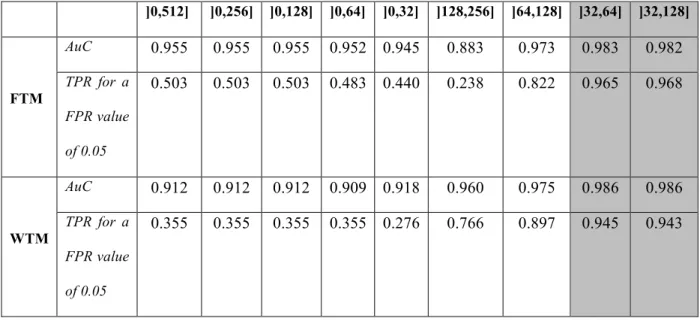
Choice of the LF band in methods FTM & WTM. We performed a sensitivity analysis with respect to

7

the choice of the LF band for FTM and WTM (2nd stage of the proposed detection method). For both 8

algorithms, the objective was to find which LF band maximizes the separation between FRs and IESs 9

in EOIs manually selected by the expert. The study was performed both on human and animal data 10

(data described in § 2.3.1 and 2.3.2). The results for the nine selected frequency bands are reported in 11

table 3 for human data and in table 4 for animal data. First, for both types of data, results revealed that 12

both methods showed dependency on this parameter. This was particularly true for FTM. For instance, 13

in human data (table 3), the TPR at fixed FPR = 0.05 was found to vary from 0.238 (LF = ]128, 256] 14

Hz) to 0.968 (LF = ]32, 128] Hz). The same result also held for mouse data. Second, the performance 15

of FTM was found to be comparable to that WTM w.r.t. the choice of LF when parameter AuC was 16

considered. Stronger differences were observed when one considers the second criterion (TPR at fixed 17

FPR = 0.05). Interestingly, the performance of WTM was found to dramatically decrease when the LF 18

band included very low frequencies (lowest performance obtained for LF = ]0, 32] Hz for human and 19

animal data). Finally, both methods exhibited best results for ]32-64] Hz and ]32-128] Hz bands with 20

an AuC almost equal to 0.99 (see grey boxes in tables 3 and 4). WTM had similar performance than 21

FTM in term of AuC but slightly lower performance (0.94 vs. 0.96 for both human and animal data) in 22

term of TPR for a FPR fixed at 0.05. This result could be explained by a detailed analysis of the ROC 23

curves which showed that, for FTM, the TPR increased in a steep manner at low FPR (2 to 5 %) but 24

reached the value of 1 for higher values. These results led us to choose the band ]32, 128] Hz as the 25

LF band to estimate the occurrence times of FRs (see eq. 2 and eq. 3) in simulated and real signals, as 26

reported hereafter. 27

1

Data Method Class

Closest Gaussian distribution

Kolmogorov test (Normal law)

Mean Variance Significance level Result Human FTM FR 0.06897 0.00083 0.05 Positive IES 0.00707 0.00010 0.05 Positive WTM FR 0.04047 0.00009 0.05 Positive IES 0.01048 0.00005 0.05 Positive Animal FTM FR 0.08900 0.00225 0.05 Positive IES 0.00638 0.00010 0.05 Positive WTM FR 0.09333 0.00058 0.05 Positive IES 0.02374 0.00021 0.05 Positive 2

Table 2: Estimated mean and variance of the FTM and WTM criteria, and results of the Kolmogorov test.

3 4 ]0,512] ]0,256] ]0,128] ]0,64] ]0,32] ]128,256] ]64,128] ]32,64] ]32,128] FTM AuC 0.955 0.955 0.955 0.952 0.945 0.883 0.973 0.983 0.982 TPR for a FPR value of 0.05 0.503 0.503 0.503 0.483 0.440 0.238 0.822 0.965 0.968 WTM AuC _{0.912 0.912 0.912 0.909 0.918 0.960 0.975 0.986 0.986} TPR for a FPR value of 0.05 0.355 0.355 0.355 0.355 0.276 0.766 0.897 0.945 0.943 5

Table 3: Human data (TLE, hippocampus). Influence of the choice of the LF band in FTM and WTM. Both

6

methods show best performance for the 32-128 Hz and 32-64 Hz bands. Gray boxes indicate best performance.

7

See glossary for abbreviations.

8 9

Threshold analysis of FTM and WTM

10

We give in table 2 the mean and variance of FTM and WTM criteria as well as the result of the 11

Kolmogarov test. We divided results between human and animal data. We found that all the 12

distributions were Gaussian and that the mean value of FRs was always greater than the mean values 13

of IES. Moreover, these mean values of the criteria do not differ so much from human to animal data 14

(0.07 and 0.09 for FTM, and 0.04 and 0.09 for WTM). From these estimated Gaussian distributions 15

the optimal threshold and the related good detection rate as a function of the FR rate are given in 1

figure 5. We found that the optimal threshold did not vary significantly for FR rate ranged from 0.1 to 2

0.9. The related good classification rates was high (>0.93) when the optimal threshold was computed 3

from a known FR rate. This good classification rates remained high (>0.9) when the optimal threshold 4

was computed from FR rate arbitrarily set to 0.5. 5 6 ]0,512] ]0,256] ]0,128] ]0,64] ]0,32] ]128,256] ]64,128] ]32,64] ]32,128] FTM AuC _{0.835 0.835 0.836 0.832 0.818 0.956 0.987 0.990 0.991} TPR for a FPR value of 0.05 0.588 0.592 0.592 0.579 0.542 0.693 0.920 0.935 0.964 WTM AuC 0.896 0.896 0.896 0.898 0.899 0.988 0.990 0.994 0.995 TPR for a FPR value of 0.05 0.788 0.788 0.791 0.798 0.740 0.939 0.977 0.941 0.945 7

Table 4: Animal data (mouse, kainate model of TLE, hippocampus). Influence of the choice of the LF band in

8

FTM and WTM. Both methods show best performance for the 32-128 Hz and 32-64 Hz bands. Gray boxes

9

indicate best performance. See glossary for abbreviations.

10 11

12

Figure 5: Optimal threshold and good classification rate of the methods as a function of the occurrence rate of

13

fast ripples. For each graph, on top is the optimal threshold as a function the fast ripple rate. On the bottom is the

good classification rate associated with this optimal threshold (solid line), and the good classification associated

1

with a threshold determined as if the fast ripple rate was equal to 0.5 (dashed line). A. Human data and FTM

2

method. B. Human data and WTM. C. Animal data and FTM. D. Animal data and WTM.

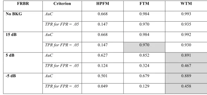
3 product. 4 5 FRBR Criterion HPFM FTM WTM No BKG AuC 0.668 0.984 0.993 TPR for FPR = .05 0.147 0.970 0.935 15 dB AuC 0.668 0.984 0.992 TPR for FPR = .05 0.147 0.970 0.930 5 dB AuC 0.627 0.852 0.891 TPR for FPR = .05 0.124 0.324 0.467 -5 dB AuC 0.501 0.679 0.889 TPR for FPR = .05 0.049 0.129 0.458 6

Table 5: Influence of the FRBR on the performance of HPFM, FTM and WTM. HPFM exhibits low AuC for all

7

values of FRBR indicating a conceptual inability of the method for distinguishing FRs from IES. For FTM and

8

WTM, the AuC decreases with the FRBR. WTM is more robust for low FRBR. Gray boxes indicate best

9

performance. See glossary for abbreviation.

10 11

Simulated signals. We compared the performance of the three methods (HPFM, FTM and WTM)

12

using signals simulated as described in section 2.3.3. The interesting aspect of such simulations is that 13

the level of background activity, characterized by the FRBR, could be varied. Results are given in 14

Table 5. First, they revealed that the HPFM exhibited very low performance whatever the level of 15

background activity relative to that of EOIs to be detected. This means that a simple high-pass filtering 16

procedure could not discriminate FRs from IESs. In other word, this result showed that the signal 17

energy beyond 256 Hz could not be used alone as a criterion to detect FRs. Second, results also 18

showed that FTM and WTM exhibited comparable results for a FRBR equal to 15 dB (which 19

corresponded to the value estimated from real data): in both cases, the AuC was found to be high 20

(>0.98) as was TPR (> 0.93) for a fixed FPR equal to 0.05. As expected, when the amplitude of EOIs 21

to be detected became low w.r.t. the amplitude of background activity (FRBR = 5 dB and FRBR = -5 22

dB), the performance of both methods decreased. Interestingly, WTM showed higher robustness w.r.t. 1

this parameter (AuC = 0.889 and TPR = 0.458) compared to FTM (AuC = 0.679 and TPR = 0.129) in 2

a situation where EOIs were (almost) impossible to detect visually (FRBR = -5dB). This result can be 3

explained by the use of a mother wavelet in WTM which shape is close to that of actual FRs in the 4

256-512Hz band. This “shape fitting” allows for changes that can still be detected in the convolution 5

6

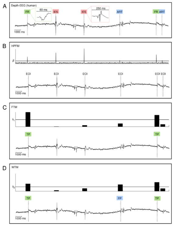
Figure 6: Behavior of proposed methods on real human data (A). The short-time energy in the 256-512 Hz band

7

(B) shows peaks at occurrence times of EOIs, which can be either FRs, IESs or artifacts. (C) Fourier Transform

8

based method. Top: ratio between energies in the 256-512 Hz band and in the 32-128 Hz band. Bottom: detection

results after thresholding. (D) Wavelet Transform based method. Top: ratio between energies in the 256-512 Hz

1

band and in the 32-128 Hz band. Bottom: detection results after thresholding. For both methods, the two 2

FRs are properly detected (true positives, TP). Note that some false positives (FP) can always be present (as for

3

WTM in this example). See glossary for abbreviations.

4 5

Real signals. Figure 6 provides a typical example showing the behaviour of the studied methods

6

(HPFM, FTM and WTM). A 20 second segment of human data (Figure 6A, see also section 2.1.1) was 7

used for this purpose. The first stage of the detection procedure is illustrated in figure 6B where the 8

signal energy in the 256-512 Hz band is plotted as a function of time. Very clear and sharp spikes 9

appeared at the time instants where EOIs (defined as events exhibiting energy in the HF band) were 10

present in the depth-EEG signal. This segment was chosen for the presence of three types of EOIs (see 11

FR, IES and ART labels in Figure 6A). In the first stage of the detection procedure, HPFM makes use 12

of a threshold

!

= 1.5 (corresponding to 0.98 percentile) to extract EOIs (marked on the signal by a 13

vertical line). For the second stage, the behaviour of FTM is displayed in Figure 6C where we 14

represented the criterion value (i.e. HF/LF

( )

FTM

E

_!

p

) for each EOI detected by HPFM at the first stage. 15

Detection results were obtained for a threshold value equal to "1 = 0.030. In this example, FTM 16

detected both FRs (marked as True Positive (TP)) and did not exhibit false detection (FP) since the 17

two IESs and the two artifacts were rejected. Finally, results obtained with WTM are displayed in 18

figure 5C. In this example, using a threshold value equal to "2 = 0.025, the method could detect both 19

FRs (as wanted) but also exhibited a false positive. 20

Quasi-simultaneous FRs and IESs. We implemented both methods in a user-friendly software that

21

allows for direct visual assessment of the detector performance on real data. The graphical user 22

interface is illustrated in figure 7A. It includes two plots showing the raw signal (upper plot, black 23

color) and the same signal (lower plot, red color) on top of which automatically detected EOIs are 24

marked by vertical bars (FRs: green color, IES: blue color). This GUI offers strong magnification on 25

EOIs for careful visual inspection of detection results, as illustrated in figure 7B. In this example, one 26

can observe the behaviour of the proposed detection method (here FTM) in the case where both the 27

IES and the FR occur quasi-simultaneously (a few tens of ms delay). Interestingly, the detector is able 28

to automatically mark both events when the duration N of the sliding Hanning window used in the first 1

stage of the detection procedure is short enough (32 ms in this case). 2

3

Figure 7: Implementation of the proposed detector (FTM) in a user-friendly software specifically designed to

4

directly inspect detection results. (A) The user selected in the EEG reviewing software (not shown) a segment of

5

about 224 s of data (upper plot). Detection results appear directly on the signal (lower plot, red trace) as green

6

bars (FRs) or blue bars (IESs). (B) A zoom on a 3 s segment of signal (upper plot). In this segment, FRs (green

7

arrows) and mixed IESs/FRs (bleu/green arrows) occur. As seen in detection results (lower plot), all FRs are

8

detected. In addition, two bars (blue and green) are automatically positioned by the detector in the presence of

9

quasi-simultaneous IESs and FRs.

10

4.

Discussion and perspectives

11

The detection of transient events in EEG signals has long been a topic of large interest in clinical 12

neurophysiology. This problem has been - and is still - considered as a difficult problem in signal 13

processing. During the past decades, many methods were proposed to automatically detect interictal 14

epileptic spikes (IESs), starting from pioneering works of Gotman (Gotman and Gloor, 1976). 1

Proposed algorithms were based on Fourier or wavelet transforms, on mimetic and rule-based 2

approaches, on neural networks, on adaptive filtering (template matching), on principal or independent 3

component analysis. Readers may refer to (Gotman, 1999) and to (Fleureau et al., 2011a; Tzallas et al., 4

2006) for partial reviews. 5

Recently, fast ripples (FRs) have attracted a lot of attention since they could constitute an interictal 6

electrophysiological marker for epilepsy (Engel et al., 2009; Jefferys et al., 2012). Indeed, FRs might 7

prove more specific than IESs with respect to the underlying epileptogenicity (Demont-Guignard et 8

al., 2012) and might be more specifically generated in brain structures involved at the onset of seizures 9

(Zijlmans et al., 2009). In this context, the reliable detection of fast ripples (FRs) can provide 10

additional and quantified arguments to epileptologists to assess the epileptogenic nature of some brain 11

structures explored with intracranial electrodes. 12

Conversely to IESs, very few methods have been proposed so far to automatically and specifically 13

detect FRs in EEG signals. This is the issue we addressed in this study. To proceed, we proposed a 14

novel detection procedure based on two stages (global detection of EOIs and local classification). The 15

evaluation methodology was based on the simulation of long-duration depth-EEG signals and on ROC 16

curves. Finally, tests were performed on real data recorded either in a patient with TLE or in an animal 17

model of TLE. 18

The main findings of this study are summarized hereafter, first from a methodological viewpoint, and 19

then from a clinical viewpoint. 20

The use of simulated signals. We decided to start from realistic simulations of depth-EEG signals.

21

Simulated signals were obtained from the insertion of real EOIs (namely FRs and IESs) into 22

background EEG activity generated from a neural mass model published elsewhere (Wendling et al., 23

2002). This approach provided a “ground truth” on both the occurrence time and the type of EOIs that 24

is crucial in the objective assessment of any detection procedure. In addition, this approach also 25

allowed us to test an important factor that was not tested in previous reports (Gardner et al., 2007; 26

Staba et al., 2002; Zelmann et al., 2012): the detection robustness when the amplitude of background 27

EEG becomes predominant w.r.t. the amplitude of EOIs to be detected. 28

A two-stage detection procedure. The basic principle of the proposed method is to first perform a

1

global detection of EOIs (defined as transient events leading to an increase of signal energy within the 2

256-512 Hz frequency band) and then perform a local analysis to assign each EOI to a specific class 3

(FR vs. IES or artifacts). We found that the combination of the two stages could bring an appropriate 4

solution to the problem of automatically identifying FRs in depth-EEG signals. The first stage consists 5

of a classical high-pass filtering (cut-off frequency: 256 Hz). It could be achieved using any filter 6

(either infinite or finite impulse response) as we found that detection results were independent from 7

the filter design procedure. It is worth mentioning that this first stage is also inspired from a current 8

practice in EEG analysis. Indeed, high-pass filtering of EEG signals (available on most EEG 9

reviewing softwares) is classically used by epileptologists to get rid of the background activity and to 10

better reveal some signal oscillations occurring in the frequency band of interest, typically the high-11

frequency band. However, it should be also reminded that both FRs and sharp transients (like IESs) 12

both lead to such oscillations in the 250-500 Hz (“fast ripples” vs. “false ripples”), as demonstrated in 13

(Benar et al., 2010). In our method, the first stage is complemented by a second stage which makes use 14

of the energy distribution (in the frequency domain) of the signal to classify EOIs. Two variants were 15

proposed for this second stage, either based on the Fourier (FT) or the Wavelet (WT) Transform. 16

These two transforms were used to compute a crucial parameter for distinguishing FRs from other 17

EOIs: the energy ratio between high frequency (HF, 250-500 Hz) and low frequency (LF) bands. The 18

choice for the LF band is discussed below (see § Parameters to be adjusted). A comparable procedure 19

was proposed in (Blanco et al., 2010) where a data mining procedure is used on candidate HFO events 20

detected by a high-pass filtering procedure (Staba et al., 2002). This unsupervised data mining 21

provides several classes that allow for the discrimination of different kinds of HFOs and artifacts. 22

While the method is very effective to achieve this goal, it looks like it requires more effort for 23

implementation compared to our method and is probably more demanding in term of computing time. 24

In addition, although unsupervised, training sets are necessary which is not the case in our method. 25

Besides, the issue of IES and IES superimposed with FRs was not addressed by the authors. In this 26

respect, our intent was different as we specifically addressed the “false ripples” issue due to sharp 27

transients (IES) (Benar et al., 2010). In addition, our method is conceptually simple. In practice, it is 1

easy to implement and use. 2

Specificity and sensitivity. The method was found to show slightly improved performance when the

3

WT is used for the second stage. In all studied situations, results showed that the use of the FT or the 4

WT for the second stage lead to a much higher performance compared to the use of a simple high-pass 5

filter. Using the WT, the method could achieve the detection of FRs with sensitivity greater to 0.93 6

when the specificity was set to 0.95. In other words, in a situation where 95% of detected EOIs are 7

actually FRs, only 7% of these EOIs are missed (either undetected or wrongly labeled) by the 8

proposed method. As expected, we also found that the method performance depends on the amplitude 9

of FRs respective to the level of background activity. As the “fast ripple to background” ratio (FRBR) 10

decreased, the method sensitivity rapidly dropped when high specificity was maintained. However, it 11

should be noted that the poorer performance (45.8% sensitivity) was obtained in a situation where the 12

FRBR was so low (- 5 dB) that FRs became undetectable by visual inspection. 13

Parameters to be adjusted. An interesting feature of the proposed method is that the number of

14

parameters to be adjusted is rather limited. For the first stage, any band pass filter (250-600 Hz) can be 15

used to compute the signal energy in the FR frequency band and then to obtain EOIs by thresholding 16

(parameter !). For the purpose of this study, we used a 4th order Butterworth filter with cut-off 17

frequencies equal to 256 Hz and 512 Hz to have a correspondence with the FTM and the WTM. An 18

IIR implementation (recursive filter) was preferred for its rapidity. Parameter ! can be easily adjusted 19

from the empirical histogram of the filtered signal energy values (see §2.2.2). For the second stage of 20

the detection procedure, the essential parameter to distinguish FRs from IESs was found to be the 21

energy ratio between high and low frequency bands (HF and LF, respectively). The HF band must be 22

adjusted to best match the frequency band of FRs (typically, 250-600 Hz). In this study, we used a HF 23

band ranging from 256 Hz to 512 Hz, constrained by the dyadic discrete wavelet transform. We let the 24

LF band as a free parameter and obtained the best results (in term of separation of FRs from IESs) for 25

a LF band equal to [32-128 Hz] which coincided with the gamma frequency band on the EEG. This 26

result also indicates that our method is likely to not be affected by slow waves (typically in the delta 27

frequency band) which can be present in EEG signals during sleep, in particular. 28

Finally, for the WTM, the mother wavelet and the number of levels must also be adjusted. We tested 1

several configurations (data not shown). Best results were obtained for a Daubechies 4 wavelet 2

decomposition on eight or nine levels depending on the sampling frequency (1024 and 2048 Hz, 3

respectively). The classification of FRs and IESs is done by thresholding the energy ratio between 4

high and low frequency bands. Interestingly, one can notice that these values do not differ so much 5

from one recording to another (same order of magnitude). This result indicates that the energy 6

distribution in proposed sub-bands (gamma and FR) is robust with respect to the type of recording 7

(performed in humans and in mice) and suggests that the algorithm can be used in some other 8

situations (like other experimental models of epilepsy) characterized by the occurrence of HFOs in the 9

FR frequency band (HF subband). 10

Potential clinical value. Both methods are relatively easy to implement. Besides the performance

11

study (in term of recognition of FRs and IESs), we could also analyse more difficult situations where 12

genuine FRs occur quasi-simultaneously with, or are part of, IESs. Indeed, the co-occurence of spikes 13

and fast ripples (denoting different pathological condition of underlying neuronal systems) can be 14

encountered and consequently is also relevant to detect. . Interestingly, for appropriate setting of the 15

time window used in the first stage, and given that both types of events do not occur strictly at the 16

same time, our method can still separate them. More generally, in most of epilepsy surgery units, 17

recordings are performed in patients candidate to surgery using long-term video-EEG monitoring (8-18

24 hours a day, 5-10 days). Huge data sets are generated by the acquisition systems since signals are 19

generally recorded on 128 to 256 channels at 1 kHz. We think that the proposed detection method can 20

dramatically decrease the workload in assessing the presence of FRs in these intracranial EEGs. In 21

addition, it may allow for systematic identification of FRs during interictal periods which represent 22

large amounts of data compared to seizure episodes. To us, it is clear that the therapeutic strategy 23

cannot depend only of the presence/absence of high frequency oscillations (HFOs) in explored brain 24

structures. However, the objective quantification of HFOs over interictal periods can efficiently 25

complement the classical often qualitative way of analyzing depth-EEG data recorded in patients with 26

drug-resistant epilepsy. 27