Deep learning models for the perception of human social interactions

Deep Learning Models for the Perception of

Human Social Interactions

by

Elizabeth Merritt Eastman

Submitted to the Department of Electrical Engineering and Computer

Science

in partial fulfillment of the requirements for the degree of

Master of Engineering in Computer Science and Engineering

at the

MASSACHUSETTS INSTITUTE OF TECHNOLOGY

June 2019

c

Massachusetts Institute of Technology 2019. All rights reserved.

Author . . . .

Department of Electrical Engineering and Computer Science

May 24, 2019

Certified by . . . .

Nancy Kanwisher

Professor Brain and Cognitive Sciences

Thesis Supervisor

Accepted by . . . .

Katrina LaCurts

Chair, Masters of Engineering Thesis Committee

Deep Learning Models for the Perception of Human Social

Interactions

by

Elizabeth Merritt Eastman

Submitted to the Department of Electrical Engineering and Computer Science on May 24, 2019, in partial fulfillment of the

requirements for the degree of

Master of Engineering in Computer Science and Engineering

Abstract

Social interaction perception is an important part of humans’ visual experience. How-ever, little is known about the way the human brain processes visual input in order to understand social interactions. In comparison, other vision problems, such as object recognition tasks, have been studied extensively and seen success by comparing state of the art computer vision models to neuroimaging data. In this thesis, I employ a similar method in order to study social interaction perception with deep learning models and magnetoencephalography (MEG) data. Specifically, I implement different deep learning computer vision models and test their performance on a social inter-action detection task as well as their match to neural data from the same task. I find that detecting social interactions most likely requires extensive cortical process-ing and/or recurrent computations. In addition, I find that experience with action recognition does not improve social interaction detection.

Thesis Supervisor: Nancy Kanwisher

Contents

1 Introduction 15

2 Related Works 19

2.1 Recognizing Social Interactions . . . 19

2.1.1 The Neural Dynamics of Social Interaction Recognition . . . . 20

2.2 Deep Neural Networks . . . 20

2.3 Comparing Convolutional Neural Networks to Brain Representations 21 2.3.1 The Merit of Comparing Convolutional Neural Networks to Brain Representations . . . 22

2.3.2 A Method for Comparing Convolutional Neural Networks and Neural Responses: Representational Similarity Analysis . . . . 23

3 Methods 25 3.1 Experimental Tasks . . . 27

3.1.1 Test Social Interaction Dataset: Social and Non Social Interac-tion Image Dataset . . . 27

3.1.2 Social Interaction Detection . . . 28

3.1.3 Match to Neural Data . . . 29

3.2 Convolutional Neural Network Models . . . 29

3.2.1 VGG-16 . . . 30

3.2.2 ResNet-50 . . . 30

3.2.3 Layers Used . . . 32

3.3.1 Object Recognition: ImageNet . . . 33

3.3.2 Action Recognition: Moments in Time . . . 33

3.3.3 Backpropagation for Fine-Tuning . . . 34

3.4 Model Dimensionality Reduction Using Principal Component Analysis 35 4 Results 39 4.1 Social Interaction Detection . . . 39

4.1.1 FF Obj . . . 39

4.1.2 FF Act . . . 39

4.1.3 RN Obj . . . 41

4.1.4 RN Act . . . 43

4.2 Match to human neural data . . . 44

5 Discussion 45 5.1 Feedforward Computations are Not Sufficient for Social Interaction Detection . . . 45

5.2 Deep Residual Networks Can Detect Social Interactions . . . 46

5.3 Deep Residual Networks Provide Better Match to MEG Data . . . . 46

5.4 The Role of Network Training: Object Recognition vs Action Recognition 47 6 Conclusion 49 6.1 Contributions . . . 49

6.2 Future Work . . . 50

A Figures 51

List of Figures

2-1 Social Interaction Detection with MEG Data: Isik et al. found that the human brain detects social interactions slowly relative to other types of visual detection, at around 300 ms [11]. . . 21

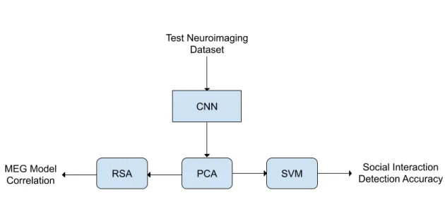
3-1 Model Architecture: This is a high level overview of the model architecture that evaluates how neural networks differentiate between social and non social interactions. The test social interaction dataset is the input to the CNN, either VGG-16 or ResNet-50. The output layers then go through PCA, or not (see Appendix A). To evaluate model performance, an SVM is trained on the model output to detect social interactions in the test images. To assess the model’s match to neural data, the output of the PCA is put through RSA to compare to the MEG data. . . 25

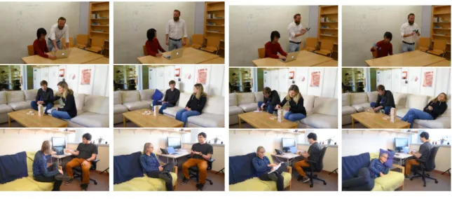
3-2 Test Social Interaction Dataset Images Each image for three of thirteen scenes is shown. In each scene there are the two different types of social interactions (a) and independent actions (b). . . 27

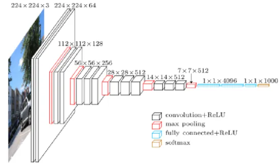
3-3 16 Network Representation of the 16 architecture. VGG-16 CNN performs spatial pooling across five max-pooling layers of stride two, following a convolutional layer. . . 30

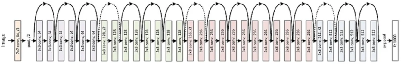
3-4 Residual Network: The basic network architecture for a ResNet with 34 blocks. Each colored block of layers represent a series of convolutions with the same dimension. The feature mapping is periodically down sampled by strided convolution. This also has an increase in channel depth in order to preserve the time complexity at each layer. Dotted lines denote residual connections. [12] . . . 31

3-5 Residual Block: Representation of a single ResNet residual block for ResNet-50 architecture. Replacing each two layer residual block with a three layer block, which uses 1x1 convolutions to reduce and subse-quently restore the channel depth, yields the ResNet-50 architecture [12]. . . 31

3-6 ResNet vs. RNN: This figure from [19] shows the formal equivalence of a ResNet with weight sharing and an recurrent neural networks (RNN). I is the identity operator. K denotes the operator that is a nonlinear transformation. . . 32

3-7 Percent Cumulative Variance Explained The cumulative variance explained for the first pooling layer of the VGG-16 network pre-trained on ImageNet. The red line shows the threshold of 99% explained. This criteria was used to decide to select the top 50 components for each model. . . 36

4-1 Results of FF Obj The classification accuracy for the output of each layer of interest in the invariant social interaction detection task for the VGG-16 model trained on an object recognition task using the top 50 components. The error bars indicate the standard deviation across 20 trials. No layers yielded significantly above chance detection performance. . . 40

4-2 Results of FF Act The classification accuracy for the output of each layer of interest in the invariant social interaction detection task for the VGG-16 model trained on an action recognition task using the top 50 components. The error bars indicate the standard deviation across 20 trials. No layers yielded significantly above chance detection performance. . . 41 4-3 Results of RN Obj The classification accuracy for the output of each

layer of interest in the invariant social interaction detection task for the ResNet-50 model trained on an object recognition task using the top 50 components. The error bars indicate the standard deviation across 20 trials. Four asterisks denotes p-value < 0.0001. . . 42 4-4 Results of RN Act The classification accuracy for the output of each

layer of interest in the invariant social interaction detection task for the ResNet-50 model trained on an object recognition task and fine-tuned on an action recognition task using the top 50 components. The error bars indicate the standard deviation across 20 trials. Three asterisks indicate p-value < 0.001. . . 43 4-5 Comparison of Four Models to MEG Correlation (rho) between

the last layers of all four models to the MEG data over time (relative to image onset). . . 44

A-1 Results of FF Obj Here the bar plot shows the results of the classi-fication accuracy for the output of each layer of interest in the social interaction detection task for the VGG16 model trained on an object recognition task. The blue bars indicate accuracy for a random 0.2 train/test split. The orange bars indicate the results for holding two scenes out. The error bars indicate the standard deviation across 20 trials. Single asterisks indicate p-value < 0.05 and two asterisks indi-cate p-value < 0.01. . . 52

A-2 Results of FF Act Here the bar plot shows the results of the classi-fication accuracy for the output of each layer of interest in the social interaction detection task for the VGG16 model trained on an object recognition task. The blue bars indicate accuracy for a random 0.2 train/test split. The orange bars indicate the results for holding two scenes out. The error bars indicate the standard deviation across 20 trials. No layers were statistically significant; all p-values were greater than 0.5 . . . 52 A-3 Results of RN Obj Here the bar plot shows the results of the

clas-sification accuracy for the output of each layer of interest in the social interaction detection task for the ResNet 50 model trained on an ob-ject recognition task. The blue bars indicate accuracy for a random 0.2 train/test split. The orange bars indicate the results for holding two scenes out. The error bars indicate the standard deviation across 20 trials. Single asterisks indicate p-value < 0.05, two asterisks indi-cate p-value < 0.01, three asterisks indiindi-cate p-value < 0.001, and four asterisks indicate p-value < 0.0001. . . 53 A-4 Results of RN Act Here the bar plot shows the results of the

clas-sification accuracy for the output of each layer of interest in the social interaction detection task for the ResNet 50 model trained on an ob-ject recognition task and fine tuned on an action recognition task. The blue bars indicate accuracy for a random 0.2 train/test split. The or-ange bars indicate the results for holding two scenes out. The error bars indicate the standard deviation across 20 trials. Single asterisks indicate p-value < 0.05, two asterisks indicate p-value < 0.01, three asterisks indicate p-value < 0.001, and four asterisks indicate p-value < 0.0001. . . 53 A-5 FF Models Matched to MEG The first two models output of the

A-6 RN Models Matched to MEG The second two models output of the last layer are matched to the MEG data collected. . . 54 A-7 FF Obj Models Matched to MEG All layers of the FF Obj model

(with and without PCA). . . 55 A-8 FF Act Models Matched to MEG All layers of the FF Act model

(with and without PCA). . . 55 A-9 RN Obj Models Matched to MEG All layers of the RN Obj model

(with and without PCA). . . 56 A-10 RN Act Models Matched to MEG All layers of the RN Act model

List of Tables

3.1 Four Models Used This table describes the four models used that differed in terms of their training and network architectures. There are two shallow feedforward models (FF) and two deeper ResNet models, approximating recurrent computations (RN). The models are trained on object (Obj) and action (Act) recognition tasks. . . 26 3.2 Test Social Interaction Dataset This table describes how the Test

Social Interaction Dataset of 52 images is broken up. There are 13 scenes where each scene is held constant across these four conditions: mutual gaze, joint attention, independent action 1, and independent action 2. . . 28 3.3 Cumulative Variance Explained for a Single Layer: This table

illustrates the structure of the data for a single layer of VGG-16. It is taken for the first convolutional layer in the VGG-16 architecture . . 35 3.4 Percent Variance Explained Percent variance explained by the top

50 PCA components for each model and layer/block. . . 37

B.1 P-Values for VGG16 This table shows the p-values for each layer for the FF Obj model. . . 57 B.2 P-Values for VGG16 Fine Tuned This table shows the p-values

for each layer for the FF Act model. . . 57 B.3 P-Values for ResNet 50 This table shows the p-values for each layer

B.4 P-Values for ResNet 50 Fine Tuned This table shows the p-values for each layer for the RN Act model. . . 58

Chapter 1

Introduction

Understanding social interactions is becoming increasingly important for todays Ar-tificial Intelligence systems that must recognize and interact with humans. Studying these processes in humans may provide key insights into building more intelligent computer vision systems.

The perception of human social interaction is the ability to detect and understand how agents associate with each other. Recognizing social interactions is a crucial part of the human visual experience. For example, humans can quickly and easily recognize whether two people sitting together are engaged in a social interaction or acting independently. This thesis aims to tackle the difficult question of how the human brain can quickly recognize these complex interactions.

Humans are highly attuned to others’ social interactions. The ability to recognize social interactions develops at a young age [5]. It is also shared with other primates [28] and is represented in a particular region of the human brain [8].

Although social interaction perception is a preeminent part of the human visual experience, there is still little understood about models and neuroimaging data com-pared to other aspects of visual recognition, such as object recognition.

Recent work from our group has used neuroimaging to study the neural basis of social interaction perception. Using functional MRI (fMRI), Isik et al. identified a region of the human posterior superior temporal sulcus (pSTS) that is selectively engaged when humans view social interactions [8]. This suggests that specialized

machinery and training may be required to recognize and distinguish social interac-tions.

More recent work from our group used magnetoencephalography (MEG) to study the neural dynamics of social interaction perception. They found that the human brain detects social interactions relatively slowly compared to primarily feedforward visual systems such as object, face, and scene recognition: social interaction detection occurred at 300 ms, versus 150 ms for object recognition, after image onset [11]. This suggests that social interaction perception may require extensive computations and/or recurrence beyond more straightforward feedforward processes like object recognition. In this thesis, I seek to better understand the type of computations underlying so-cial interaction perception using convolutional neural networks (CNNs). CNNs are a set of popular feedforward models in computer vision loosely inspired by the architec-ture of the brain. They have been useful for understanding the neural computations behind other aspects of vision, such as object [31] and scene recognition [2, 3].

I compare different CNNs, using their outputs, to the MEG data mentioned above in order to better understand the underlying computations. By having a model to compare MEG data, I can more explicitly test the roles of different network architec-tures. Understanding the roles of these architectures can help us compare different types of computations. In addition, we can also examine the roles of different types of visual experiences or training on the performance of these networks.

Specifically, I look at two network architectures, one shallower and one deeper, which are trained in two different ways, one is trained on a generic object recognition task and the other is trained on a more specific action recognition task. I compare these networks in terms of their (1) ability to detect social interactions in images and (2) match neural responses to the same images.

Based on the above neuroimaging studies from our group, I hypothesize that de-tecting social interactions requires: (1) extensive recurrent processing [11], and (2) specialized machinery and/or training [8]. I found that, indeed, extensive processing was needed in order to differentiate between social and non-social interactions. Spe-cialized training, however, did not improve the networks’ social interaction detection

Chapter 2

Related Works

2.1

Recognizing Social Interactions

Social interactions depend on the ability to understand the actions of multiple people and how they relate to each other. The ability to perceive and understand social interactions begins early in development [5] and is shared with other primates [28]. As mentioned in chapter 1, however, the neural computations underlying this ability are largely unknown.

Some behavioral studies that suggest the perception of social interactions shares a similar task of a classic visual pattern recognition problem: face recognition. People are better able to perceive social interactions when stimuli are presented upright, as opposed to inverted; however, the same is not true for perception of independent actions [22]. Bodies facing each other (seemingly interacting) were recognized more accurately than bodies facing away from each other (non interacting). The team saw that recognition of facing bodies, but not nonfacing bodies, was strongly impaired when those stimuli were inverted [22]. Additionally, social interactions receive pref-erential access to visual awareness [29] and facilitate visual processing of groups of individuals [30].

Recently, Isik et al. performed a study to test the sensitivity of the cortical region to the presence of social interactions. The group found that there exists sensitivity to the presence and nature of social interactions in a region of the pSTS. This sensitivity

cannot be explained by sensitivity to physical interactions or to the animacy or goals of individual agents [10, 8].

2.1.1

The Neural Dynamics of Social Interaction Recognition

MEG is a functional neuroimaging technique that measures changes in magnetic fields produced by neurons firing synchronously. The spatial distributions of the magnetic fields are analyzed in order to localize the areas of activity within the brain. MEG has ms-temporal resolution because it is a direct measure of neural firing, making it a good tool for studying neural computations. In addition, MEG is a non-invasive tool in the study of neural computations.

Recently, our group showed subjects in the MEG the images of pairs of individ-uals, or dyads, engaged in a social interaction or acting independently. This image dataset is described further in section 3.1.2. They found that the human brain can detect which images contain social interactions and which do not [11] based on the information in their MEG signals. However, this information appeared to come online slowly relative to most visual computations that are primarily feedforward: around 300 ms after image onset, as shown in 2-1. As stated in chapter 1, these results suggest that social interaction detection may require extensive recurrent processing.

2.2

Deep Neural Networks

The process by which an individual perceives his or her surroundings is an excep-tionally complex one. The task of training a machine to mimic the human visual system also carries a multitude of challenges and complexities. Specifically, image recognition is made difficult by the wide assortment of objects and the transforma-tions that change their visual appearance [23]. Given this issue of transformation, large amounts of training data may be required for models to obtain desirable per-formance. This poses a problem for the application of traditional neural networks, as large amounts of training data is required. Luckily, there exist implementations of Deep Neural Networks (DNNs) which are optimized to deal specifically with this

Figure 2-1: Social Interaction Detection with MEG Data: Isik et al. found that the human brain detects social interactions slowly relative to other types of visual detection, at around 300 ms [11].

hurdle: Convolutional Neural Networks.

Convolutional Neural Networks (CNNs) are a subset of DNNs that perform a series of convolutions (filters) on the inputted data at each layer, and are loosely inspired by the visual cortex [7]. These series of filters are performed in an effort to identify specific features or aspects of the data. For the purposes of image recognition, this is a very powerful approach because it allows one to exploit various commonalities that one might come across in normal images. The convolution implements the same filter at different positions, or scales, and then pools across these filters to provide invariance to the transformations described above [4, 18, 24]. CNNs have achieved state of the art performance on many computer vision tasks including object recognition [17, 25].

2.3

Comparing Convolutional Neural Networks to

Brain Representations

CNNs are inspired by classical theories of biological brain functions and recent work comparing CNNs to neural data for other vision problems, such as object recognition,

have been very successful [15].

Yamins et al. found that internal representations of early DNN models are ex-tremely similar to the neural representation measured experimentally in the primate brain [31]. The authors sought to find a quantitatively accurate model of the infe-rior temporal (IT) cortex in primates, which is the final layer of the ventral object recognition pathway. They found that high-performing neural networks on object recognition tasks also matched human performance and recordings from primate vi-sual cortex on the same tasks. Further, optimizing a network on an object recognition task led to a better match with the IT data [31].

Khaligh-Razavi et al. extended the above work to humans. They compared computational model representations to representations in human and monkey brains and found that the more similar a model representation was to the high-level visual brain representation, the better the model performed at object categorization [13].

More recently, Schrimpf et al., posed the question of whether or not newer CNNs with more layers were moving further away from an accurate representation of the mechanisms used in the human brain [26]. The authors developed Brain-Score which attempts to measure CNNs on how similar the models are to the brains mechanisms for core object recognition. Schrimpf et al. found that as ImageNet performance improved, a CNNs Brain-Score improved [26].

2.3.1

The Merit of Comparing Convolutional Neural

Net-works to Brain Representations

The success of CNNs in predicting neural responses has sparked a debate over whether or not CNNs are a good scientific model to understand the human brain [20]. It is important to note that the predictive power of CNNs can lead to proof of concept, and allow CNNs to be used to pursue practical aims such as experimental control. Many argue that despite their complex appearance, CNNs provide the same explanations as traditional mathematical theoretical models [20]. Further, the investigation of neutral analogies between CNNs and the brains is a promising source of new hypotheses for

empirical testing.

2.3.2

A Method for Comparing Convolutional Neural

Net-works and Neural Responses: Representational

Simi-larity Analysis

Comparing the representations of CNNs and the brain can be challenging because the output of a convolutional neural network is in a completely different space than the output of different neural recordings: classification of probabilistic values and measure of magnetic fields. In 2008, Kriegeskorte et al. proposed a framework called representational similarity analysis (RSA) to compare data across different modal-ities [16]. RSA quantitatively relates multi-channel measures of neural activity to each other and to computational theory and behavior by comparing representational dissimilarity matrices (RDMs). An RDM characterizes the information in a brain measurement or model. More specifically, an RDM is a pairwise matrix of the dis-tance between all stimuli in a dataset for each modality. The innovation of RSA was to express the neural/model response patterns in these matrices that are sized stim-ulus by stimstim-ulus, which is always the same regardless of the dimension of the input data. Utilizing RSA enables integration of computational modeling into the analysis of brain-activity data.

Chapter 3

Methods

Figure 3-1: Model Architecture: This is a high level overview of the model ar-chitecture that evaluates how neural networks differentiate between social and non social interactions. The test social interaction dataset is the input to the CNN, either VGG-16 or ResNet-50. The output layers then go through PCA, or not (see Appendix A). To evaluate model performance, an SVM is trained on the model output to detect social interactions in the test images. To assess the model’s match to neural data, the output of the PCA is put through RSA to compare to the MEG data.

Four different models were compared on the task of differentiating between images with or without social interactions. The four models consisted of two neural network architectures trained on different tasks. The first two models utilized a VGG-16

network, where one model was trained on an object recognition task and the other was fine-tuned on an action recognition task. The second two models utilized a much deeper ResNet-50 network, trained on the same object and action recognition tasks. The goal was to evaluate these networks in terms of (1) their performance on social interaction detection, and (2) how well their representations match those in the human brain as measured by MEG responses to the same images [11].

Name Description

FF Obj VGG-16 trained on object recognition task (ImageNet) FF Act VGG-16 trained on object recognition task (ImageNet) and fine-tuned on an action recognition task (Moments in Time)

RN Obj ResNet-50 trained on object recognition task (Ima-geNet)

RN Act ResNet-50 trained on object recognition task (Ima-geNet) and fine-tuned on an action recognition task (Moments in Time)

Table 3.1: Four Models Used This table describes the four models used that dif-fered in terms of their training and network architectures. There are two shallow feedforward models (FF) and two deeper ResNet models, approximating recurrent computations (RN). The models are trained on object (Obj) and action (Act) recog-nition tasks.

(a) Social Interactions (b) Non Social Interactions

Figure 3-2: Test Social Interaction Dataset Images Each image for three of thirteen scenes is shown. In each scene there are the two different types of social interactions (a) and independent actions (b).

3.1

Experimental Tasks

3.1.1

Test Social Interaction Dataset: Social and Non Social

Interaction Image Dataset

The data set used for model testing consisted 52 images taken around the MIT cam-pus. There were four different conditions that were shot across 13 scenes. Each scene contained a new pair of actors that were either engaged in a social interaction or acting independently. For social interactions, there were two sub categories: joint attention and mutual gaze. There were two different non social interactions for each scene. Thus, the dataset consisted of 26 social interaction images and 26 non-social interaction images. The dataset is further explained in table 3.2. Having the same actors and background in a given scene made this dataset very well-controlled in or-der to evaluate social interaction recognition without the influence of low-leve visual confounds.

Condition Description of Condition Type

Mutual Gaze Two people looking at each other Social interaction Joint Attention Two people looking at the same

object

Social interaction

Independent Actions 1 Two people engaged in indepen-dent actions

Non social interaction

Independent Actions 2 Two people engaged in different independent actions

Non social interaction

Table 3.2: Test Social Interaction Dataset This table describes how the Test Social Interaction Dataset of 52 images is broken up. There are 13 scenes where each scene is held constant across these four conditions: mutual gaze, joint attention, independent action 1, and independent action 2.

3.1.2

Social Interaction Detection

In order to determine if the features in each model layer can distinguish between images with versus without social interactions, a Support Vector Machine (SVM) was trained on the output of each layer to classify social and non social interactions. A linear SVM is a good method for this task as the social and non social data points should be linearly separated in order to be read out by downstream populations of neurons [23].

Invariant Social Interaction Detection

In particular, I wanted to see if the neural networks learned abstract representations of social interactions, beyond simple visual cues. For each layer, the image vectors were split into train and test data. There were two different methods of train, test split used: a standard randomize train and test split or leave specific scenes out for test split.

As described in section 3.1.1, there were four conditions (images) for each scene-three example scenes are shown in each row of Figure 3-2). In order to see if the networks generalized visually across different scenes in the Test dataset, I held two

scenes out of the SVM training. Thus, the dataset was split into training and testing data by scene, rather than random images. In the standard randomized train, test split, a scene can be shown for training, such as “scene one joint attention” and for testing, “scene one no interaction”. By splitting the training and testing data using this method, the model was required to learn an invariant representation of social interactions that could generalize across scenes.

Results using a standard 80/20 split are also reported in Appendix A. Some models showed better performance for the standard split, likely because similar images from the same scene could appear in both the train and test sets. The results reported in chapter 4 are for the main test of interest: invariant social interaction detection.

3.1.3

Match to Neural Data

To understand the neural computations underlying social interactions, I wanted to see not only how well the different networks perform on the task, but also how they compared to brain representations. The brain representation was measured by MEG and the data collection is explained in section 2.1.1. I compared the representations in each of the four neural network models to existing MEG data of subjects viewing the same Test Social Interaction Dataset as described in figure 3-2 and section 3.1.1. Specifically, I used RSA to correlate the MEG data at each time step with the output of each model layer. RSA quantitatively relates multi-channel measures of neural activity to each other and to computational theory and behavior by comparing representational dissimilarity matrices (RDMs). The output of the model is a matrix of the layer. This output was compared to the MEG data using a pairwise correlation between the model output, which remains the same, and MEG data of all subjects at each time step. This enabled me to see which of the CNN models is most comparable to MEG data.

3.2

Convolutional Neural Network Models

Figure 3-3: VGG-16 Network Representation of the VGG-16 architecture. VGG-16 CNN performs spatial pooling across five max-pooling layers of stride two, following a convolutional layer.

3.2.1

VGG-16

The VGG networks are perhaps best known for their successful results on object recognition tasks. In addition, these and similar CNN models have been shown to have good correspondence with primate neural data [26]. The VGG-16 CNN performs spatial pooling across five max-pooling layers of stride two, following a convolutional layer. Importantly, VGG-16 has more convolutional layers at the higher levels, where spatial resolution is lower, which reduces memory consumption [27]. I utilized a VGG-16 architecture, shown in figure 3-3.

3.2.2

ResNet-50

The second set of experiments involved the Residual Networks (ResNet) model first proposed by He et. al in 2016 [6]. Building on the methodology of the aforementioned VGG Networks, ResNets have displayed great success in image recognition by form-ing extremely deep graphs, with some implementations containform-ing over 150 hidden layers. The key insight of the ResNet architecture is the preservation of data repre-sentation. In other words, as CNNs get deeper, the risk of extra layers mistakenly

Figure 3-4: Residual Network: The basic network architecture for a ResNet with 34 blocks. Each colored block of layers represent a series of convolutions with the same dimension. The feature mapping is periodically down sampled by strided convolution. This also has an increase in channel depth in order to preserve the time complexity at each layer. Dotted lines denote residual connections. [12]

Figure 3-5: Residual Block: Representation of a single ResNet residual block for ResNet-50 architecture. Replacing each two layer residual block with a three layer block, which uses 1x1 convolutions to reduce and subsequently restore the channel depth, yields the ResNet-50 architecture [12].

altering an already correct representation of the data also increases. To combat this issue, Residual Networks make use of an identity function that bypasses the residual convolution of individual layers, allowing for the preservation of well-learned informa-tion. Therefore, lower layers can form a very good representation of the data. Higher layers will attempt to correct the residual error across convolutions, but otherwise copy the lower layers as they were.

The specific residual network used in this work is ResNet-50, a residual network model containing fifty layers.

ResNet is believed to be equivalent to shallow Recurrent Neural Network (RNN); it is also thought to be a good model of recurrent connections in the ventral stream [19]. Figure 3-6 shows that unrolling the feedback system gives a deep residual network with the same weights, where the number of layers that are unrolled corresponds to time

Figure 3-6: ResNet vs. RNN: This figure from [19] shows the formal equivalence of a ResNet with weight sharing and an recurrent neural networks (RNN). I is the identity operator. K denotes the operator that is a nonlinear transformation.

iterations of the dynamical system. Thus, Liao and Poggio conclude that ResNets with shared weights can be reformulated into the form of a recurrent system.

3.2.3

Layers Used

VGG-16 consists of 16 layers with learnable weights: 13 convolutional layers and three fully connected layers. The total number of parameters in the VGG-16 network architecture is 138 million [27]. ResNet-50 consists of 50 layers: 49 convolutional layers and one full connected layer. ResNet-50 contains 25 million parameters, significantly less than the number of parameters in VGG-16. Given the different number of layers and parameters in the two models, I sought to find the corresponding representations across the two networks by comparing analogous layers and dimensionality reducing the output of those layers, explained in section 3.4.

For VGG-16, I used the feature vectors produced by the five pooling layers, high-lighted in red in figure 3-3. For ResNet-50, similar to the pooling layers, I used the output, feature vectors of each of the four residual blocks. The blocks correlated with the purple, green, red, and blue layers in figure 3-4.

3.3

Network Training

The next step after constructing the models was training them on different tasks. Two datasets are utilized to train the neural network models: ImageNet and Moments in Time.

3.3.1

Object Recognition: ImageNet

ImageNet is a large-scale dataset utilized for object recognition. ImageNet samples a large number of categories and provides good within-class variability to capture different transformations. The specific ImageNet dataset used is pulled from the Large Scale Visual Recognition Challenge 2012 (ILSVRC 2012) [25]. This dataset includes 150,000 images with 1,000 object categories for validation and test data.

This acted as a “baseline” test, as ImageNet is organized according to the WordNet hierarchy, which only includes nouns, and does not have any explicit information about people or social actions.

I utilized a VGG-16 network that was pre-trained on ImageNet. In addition, I fine-tuned this network, which was previously trained on ImageNet, with the action recognition dataset. I describe fine-tuning in section 3.3.3.

3.3.2

Action Recognition: Moments in Time

The Moments in Time dataset is a very large-scale action recognition dataset utilized to recognize and understand actions and events in videos. Moments in Time is being developed by the MIT-IBM Watson AI Lab [21]. The dataset includes a collection of one million, labeled, 3-second video clips. The videos can involve people, animals, or objects, and the action categories were selected using 4,500 of the most common verbs using VerbNet [21]. Each video is labeled as one of the 339 action or activity categories defined by the Moments group. Every action, or verb, is associated with over 1,000 videos. I trained on this 339-way action recognition task, utilizing single frame images from this dataset, rather than the 3 second video clips [21].

By fine-tuning the models on the action recognition task, I can see if further training on action recognition helps in generalization in the social interaction detection task.

I utilized a ResNet-50 network that was pre-trained on ImageNet. In addition, the Moments in Time group released a fine-tuned version of their network which was previously trained on ImageNet.

3.3.3

Backpropagation for Fine-Tuning

The above models are all trained and fine-tuned using backpropagation, which enables the network to update the parameter weights. Backpropagation exploits the chain rule in order to update the weights, or parameters, of the network based on learning errors in the training data. As mentioned above, the parameters for the models consist of 138 million and 25 million for VGG-16 and ResNet-50, respectively. While FF Obj, RN Obj, and RN Act were all pre-trained/fine-tuned, I performed additional fine-tuning on FF Act using the Moments in Time dataset. To do this, I followed the same procedure outlined in [21] to fine-tune RN Act.

First, I utilized a sparse Softmax Cross Entropy loss function, taking the mean across batches. For this loss function, the probability of a given label is considered exclusive, meaning that soft classes are not allowed and the labels vector must provide a single specific index for the true class of each batch entry. The batch size is the number of training samples used to make a single update to the model parameters. It is important to combine the loss, by taking the mean, from each point in the entire batch. By taking the mean the loss is no longer dependent on the number of data points (which it would be if the sum were used instead).

Next, in order to backpropogate, the derivative of the loss is taken. Given the loss function, the model begins with the errors, derives them, and propogates back from the errors from the end to the beginning.

In addition, I utilized the Adam Optimizer to minimize the total loss minimize the total loss, with learning rate = 0.001, β1 = 0.9, and β2 = 0.999 [14]. The Adam

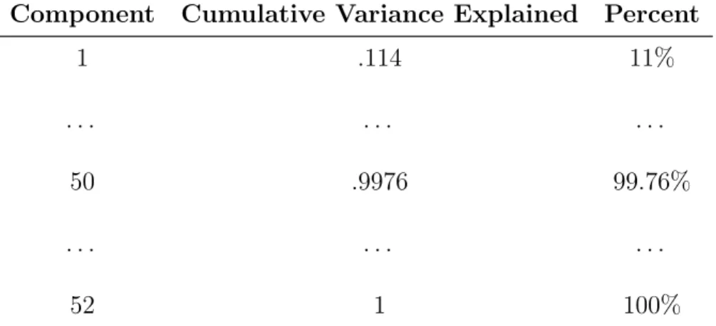
Component Cumulative Variance Explained Percent 1 .114 11% . . . . 50 .9976 99.76% . . . . 52 1 100%

Table 3.3: Cumulative Variance Explained for a Single Layer: This table illustrates the structure of the data for a single layer of VGG-16. It is taken for the first convolutional layer in the VGG-16 architecture

objective functions, based on adaptive estimates of lower-order moments [14]. The update equations for Adam are as follows:

mt= β1mt−1+ (1 − β1)Ot

vt= β2vt−1+ (1 − β2)O2t

where vt is an exponentially decaying average of past squared gradients and mt is

an exponentially decaying average of past gradients.

3.4

Model Dimensionality Reduction Using

Prin-cipal Component Analysis

In order to compare the performance of different model layers, which all have differ-ent dimensionality, I compressed the dimensions of each output layer using Principal Component Analysis (PCA). PCA is a powerful tool in data compression, using or-thogonal projections to convert observations to principal components.

My goal was to reduce the dimensionality without losing explainable variance in the data. Thus for each model layer, I looked at the percent cumulative variance explained of each component and chose the minimum number of components that

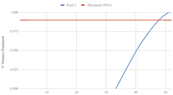
Figure 3-7: Percent Cumulative Variance Explained The cumulative variance explained for the first pooling layer of the VGG-16 network pre-trained on ImageNet. The red line shows the threshold of 99% explained. This criteria was used to decide to select the top 50 components for each model.

still explain at least 99% of the data. The results for a single layer of this procedure can be seen in table 3.3 and figure 3-7.

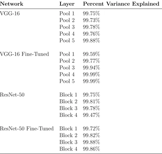
Following this procedure, the top 50 components were selected to use for the PCA portion. The percent variance explained for the top 50 components of all layers of interest are shown in table 3.4.

I also performed all experiments without using PCA. The results were almost identical and are reported in Appendix A.

Network Layer Percent Variance Explained VGG-16 Pool 1 99.75% Pool 2 99.73% Pool 3 99.78% Pool 4 99.76% Pool 5 99.88% VGG-16 Fine-Tuned Pool 1 99.59% Pool 2 99.77% Pool 3 99.94% Pool 4 99.99% Pool 5 99.99% ResNet-50 Block 1 99.75% Block 2 99.81% Block 3 99.78% Block 4 99.47% ResNet-50 Fine-Tuned Block 1 99.72% Block 2 99.82% Block 3 99.88% Block 4 99.86%

Table 3.4: Percent Variance Explained Percent variance explained by the top 50 PCA components for each model and layer/block.

Chapter 4

Results

Below, I describe the results for the four different networks outlined in chapter 3. First, there are two shallower feedforward networks trained on object and action recognition tasks, models FF Obj and FF Act, respectively. Second are the RN Obj and RN Act, two deeper residual networks, which approximate shallower recurrent networks, as discussed in section 3.2.2.

4.1

Social Interaction Detection

4.1.1

FF Obj

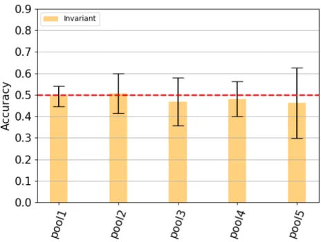
The most basic model utilized was the FF Obj, where the VGG-16 network was pre-trained on only an object recognition task. The results showed that all network layers perform at chance, figure 4-1. This was also true without PCA or using random 80-20 splits of the data, as shown in the appendix figure A-1. This implies that generic feedforward computations cannot distinguish between scenes with or without social interactions.

4.1.2

FF Act

I next asked if the VGG-16 network would perform better given more specific in-formation about human bodies and actions. To answer this question, the network,

Figure 4-1: Results of FF Obj The classification accuracy for the output of each layer of interest in the invariant social interaction detection task for the VGG-16 model trained on an object recognition task using the top 50 components. The error bars indicate the standard deviation across 20 trials. No layers yielded significantly above chance detection performance.

Figure 4-2: Results of FF Act The classification accuracy for the output of each layer of interest in the invariant social interaction detection task for the VGG-16 model trained on an action recognition task using the top 50 components. The error bars indicate the standard deviation across 20 trials. No layers yielded significantly above chance detection performance.

which was previously trained on an object recognition task, was then fine-tuned on the Moments in Time dataset, an action recognition task. This is the FF Act model. The results show that the network does not perform above chance at any layer in the model. Thus, it seems that feedforward computations, even specialized for an action recognition task, cannot distinguish between scenes with or without social interactions.

4.1.3

RN Obj

The third model is a deeper model utilizing the ResNet-50 network pre-trained on an object recognition tasks. The results show that the last block in the network performs significantly above chance at the invariant social interaction detection tasks. No earlier blocks were above chance.

Figure 4-3: Results of RN Obj The classification accuracy for the output of each layer of interest in the invariant social interaction detection task for the ResNet-50 model trained on an object recognition task using the top 50 components. The error bars indicate the standard deviation across 20 trials. Four asterisks denotes p-value < 0.0001.

Figure 4-4: Results of RN Act The classification accuracy for the output of each layer of interest in the invariant social interaction detection task for the ResNet-50 model trained on an object recognition task and fine-tuned on an action recognition task using the top 50 components. The error bars indicate the standard deviation across 20 trials. Three asterisks indicate p-value < 0.001.

4.1.4

RN Act

The fourth model, RN Act, is the same deep residual network as RN Obj, but further fine-tuned with an action recognition task. The results are very similar to those of RN Obj: the last block, but not in earlier layers, performs significantly above chance.

Figure 4-5: Comparison of Four Models to MEG Correlation (rho) between the last layers of all four models to the MEG data over time (relative to image onset).

4.2

Match to human neural data

All four models were compared to the MEG data described in section 3.1.2. For each of the four models I looked at the the last layer (or block): pool 5 in the VGG networks (FF Obj and FF Act) and block 4 in the ResNets (RN Obj and RN Act). These layers were chosen because they were the only layers that provided significantly above chance social interaction detection. The results are shown in figure 4-5.

The deep residual learning networks, RN Obj and RN Act, provide the best match to the MEG data. These results suggest that deep feedforward or recurrent networks are likely used to recognize social interactions in the human brain.

Chapter 5

Discussion

I found that very deep neural network models are required to detect social interactions in images, specifically, that only the deep residual learning networks could recognize social interactions above chance, shown in figures 4-3 and 4-4.

These deep neural networks also provided the best match to MEG data, as mea-sured by the correlation between the pattern of activity across images. Interestingly, I found that specialized training on an action recognition task did not improve per-formance or correlation to MEG data.

5.1

Feedforward Computations are Not Sufficient

for Social Interaction Detection

As shown in figure 4-1, the shallower feedforward models did not perform above chance on the invariant social interaction detection task. This supports the hypothesis that social interaction perception may require more extensive computations rather than a shallow feedforward process. In object recognition, however, there has been much success utilizing feedforward processes, including the model used here: VGG-16. Neural timing data provides a parallel explanation: in object recognition, the human brain detects an object at about 150 ms after image onset, much faster than the 300 ms required for social interaction detection [1] [9]. This delayed latency for social

interaction detection may explain why the FF Obj and FF Act models performed simply at chance.

5.2

Deep Residual Networks Can Detect Social

In-teractions

I found that the final block of both deep residual networks tested (RN Obj and RN Act) could detect social interactions in images significantly above chance, shown in figures 4-3 and 4-4. This was true even though the network was trained and tested on completely different scene/actor combinations, as described in section 3.1.2, suggesting that this detection is not due to low-level visual properties.

Utilizing a ResNet model for the second two models is important due to a Residual Network’s comparable properties to standard Recurrent Neural Networks. Liao and Poggio hypothesized that the effectiveness of most deep feedforward neural networks, including ResNet, is their ability to approximate recurrent computations [19]. These computations are prevalent in most task with larger time than shallow feedforward networks [19].

prevalent in most tasks with duration longer than shallow feedforward networks

5.3

Deep Residual Networks Provide Better Match

to MEG Data

Figures A-5, A-6, and 4-5 show how the four models correlated with the MEG data collected on human subjects. Similar to the results seen for model accuracy, the ResNet models provided the best match to the MEG data. In other words, models that perform better at social interaction detection, also provide a better match with human neural data.

Taken together, these results suggest that extensive feedforward computations, or more likely recurrence, are required to recognize social interactions. This is in

agreement with the relatively late MEG classification for social interactions compared to previously reported latencies for other types of visual pattern classification [11].

5.4

The Role of Network Training: Object

Recog-nition vs Action RecogRecog-nition

I utilized two different recognition tasks for network training: object and action recog-nition. It was my hope that training on an action recognition task would improve the models’ accuracy in detecting social interactions. These networks should have more experience with human forms and actions that are relevant for social interaction de-tection, especially because the object recognition training task (ImageNet) does not have any categories for humans or bodies [25]. However, this action training did not improve social interaction detection or match to MEG data. This is likely because the four models have all seen a wide range of natural images, and similar networks have been shown to generalize across different visual pattern recognition tasks [11]. Further, human neural data suggests that social interactions are recognized in a dedi-cated brain region distinct from those for recognizing individual actions [8]. Thus, it seems likely that a specific social action recognition task would be required to improve model performance.

Chapter 6

Conclusion

6.1

Contributions

This thesis used four deep neural network models to test the hypotheses that detecting social interactions requires: (1) extensive recurrent processing [11], and (2) specialized machinery and/or training [8]. To do this I compared the performance of different neural networks on a social interaction detection task and their match to human neural responses to the same images, as measured by MEG.

I used four different deep neural networks to ask about the nature of the com-putations underlying human social interaction detection. In particular, I looked at the role of shallow versus deep (or recurrent) network architectures, and the role of training on different tasks. I assessed the networks’ performance both in terms of their invariant social interaction detection accuracy and match to neural data.

I found that only the deep residual learning networks could recognize social inter-actions above chance, shown in figures 4-3 and 4-4, and provided a better match to the MEG data. As described in section 3.2.2, these networks are equivalent to shallower recurrent models. This is consistent with delayed social interaction recognition that occurs in the human brain [11]. I saw no improvement when training either network on an action recognition task.

These results suggest that (1) detecting social interactions most likely requires extensive cortical processing and/or recurrent computations, and (2) that experience

with action recognition does not improve social interaction detection.

6.2

Future Work

This work opens the door to many future modeling and neuroimaging studies. The first, would be to train the network explicitly on a social interaction task to see if that improves results. While I found no improvement with specialized action train-ing, action recognition tasks do not necessarily provide any new social interaction information and training on an explicit social interaction task may be required. This, of course, is limited by a lack of large-scale social interaction datasets. As a step in this direction, I have labeled action categories from the Moments in Time dataset as social or non-social actions. Training on these specified actions could lead to improved accuracy on the ResNet-50 model.

In addition, while we find that the ResNet models outperform the shallower VGG networks, we cannot disambiguate between extensive feedforward and recurrent pro-cessing in the brain. Further, neuroimaging experiments combining high spatial reso-lution of fMRI and high temporal resoreso-lution of MEG, can be done to help disambigute between feedforward/recurrent processing of social interactions.

Finally, this work is important for establishing a framework for more computa-tional studies of social interaction detection. By applying the computer vision tools from successful studies focused on object, scene, and action recognition, we can begin to understand the neural computations underlying different aspects of social visual perception.

Appendix A

Figures

(a) VGG-16 network pretrained on ImageNet results

(b) VGG-16 pretrained on ImageNet with the top 50 components results

Figure A-1: Results of FF Obj Here the bar plot shows the results of the clas-sification accuracy for the output of each layer of interest in the social interaction detection task for the VGG16 model trained on an object recognition task. The blue bars indicate accuracy for a random 0.2 train/test split. The orange bars indicate the results for holding two scenes out. The error bars indicate the standard deviation across 20 trials. Single asterisks indicate p-value < 0.05 and two asterisks indicate p-value < 0.01.

(a) VGG-16 network pretrained on ImageNet results and fine tuned on Moments in Time

(b) VGG-16 fine tuned on Moments in Time with the top 50 components results

Figure A-2: Results of FF Act Here the bar plot shows the results of the clas-sification accuracy for the output of each layer of interest in the social interaction detection task for the VGG16 model trained on an object recognition task. The blue bars indicate accuracy for a random 0.2 train/test split. The orange bars indicate the results for holding two scenes out. The error bars indicate the standard deviation across 20 trials. No layers were statistically significant; all p-values were greater than 0.5

(a) ResNet 50 network pretrained on Ima-geNet Results

(b) ResNet 50 pretrained on ImageNet with the top 50 components results

Figure A-3: Results of RN Obj Here the bar plot shows the results of the classifica-tion accuracy for the output of each layer of interest in the social interacclassifica-tion detecclassifica-tion task for the ResNet 50 model trained on an object recognition task. The blue bars in-dicate accuracy for a random 0.2 train/test split. The orange bars inin-dicate the results for holding two scenes out. The error bars indicate the standard deviation across 20 trials. Single asterisks indicate p-value < 0.05, two asterisks indicate p-value < 0.01, three asterisks indicate p-value < 0.001, and four asterisks indicate p-value < 0.0001.

(a) ResNet 50 network pretrained on Ima-geNet and fine tuned on Moments in Time results

(b) ResNet 50 pretrained on ImageNet and fine tuned on Moments in Time with the top 50 components results

Figure A-4: Results of RN Act Here the bar plot shows the results of the clas-sification accuracy for the output of each layer of interest in the social interaction detection task for the ResNet 50 model trained on an object recognition task and fine tuned on an action recognition task. The blue bars indicate accuracy for a random 0.2 train/test split. The orange bars indicate the results for holding two scenes out. The error bars indicate the standard deviation across 20 trials. Single asterisks indicate p-value < 0.05, two asterisks indicate p-value < 0.01, three asterisks indicate p-value < 0.001, and four asterisks indicate p-value < 0.0001.

(a) VGG16 network pretrained on ImageNet with and without PCA

(b) VGG16 fine tuned on Moments in Time with and without PCA

Figure A-5: FF Models Matched to MEG The first two models output of the last layer are matched to the MEG data collected.

(a) ResNet 50 network pretrained on Ima-geNet with and without PCA

(b) ResNet 50 fine tuned on Moments in Time with and without PCA

Figure A-6: RN Models Matched to MEG The second two models output of the last layer are matched to the MEG data collected.

(a) VGG 16 trained on object recognition task

(b) VGG 16 trained on object recognition with PCA

Figure A-7: FF Obj Models Matched to MEG All layers of the FF Obj model (with and without PCA).

(a) VGG16 fine tuned on action recognition task

(b) VGG16 fine tuned on action recognition with PCA

Figure A-8: FF Act Models Matched to MEG All layers of the FF Act model (with and without PCA).

(a) ResNet 50 trained on object recognition task

(b) ResNet 50 trained on object recognition with PCA

Figure A-9: RN Obj Models Matched to MEG All layers of the RN Obj model (with and without PCA).

(a) ResNet 50 fine tuned on action recogni-tion task

(b) ResNet 50 fine tuned on action recogni-tion with PCA

Figure A-10: RN Act Models Matched to MEG All layers of the RN Act model (with and without PCA).

Appendix B

Tables

VGG16 80/20 Split with PCA Hold 2 Scenes Out with PCA

Pool 1 .433 .025 .5 .287

Pool 2 .370 .423 .387 .385

Pool 3 .005 .051 .5 .114

Pool 4 .006 .061 .127 .162

Pool 5 .332 .5 .169 .162

Table B.1: P-Values for VGG16 This table shows the p-values for each layer for the FF Obj model.

VGG16 FT 80/20 Split with PCA Hold 2 Scenes Out with PCA

Pool 1 .063 .13 .048 .006

Pool 2 .07 .001 .008 .145

Pool 3 .0041 .001 .031 .031

Pool 4 .00017 .001 .0156 .004

Pool 5 5.08e-06 5.08e-06 .287 .287

Table B.2: P-Values for VGG16 Fine Tuned This table shows the p-values for each layer for the FF Act model.

ResNet 50 80/20 Split with PCA Hold 2 Scenes Out with PCA

Block 1 .0007 .0007 .011 .063

Block 2 .043 .037 .420 .346

Block 3 .015 .011 .031 .245

Block 4 .130 .077 .001 6.38e-08

Table B.3: P-Values for ResNet 50 This table shows the p-values for each layer for the RN Obj model.

ResNet 50 FT 80/20 Split with PCA Hold 2 Scenes Out with PCA

Block 1 .0056 .0021 .407 .412

Block 2 .055 .0298 .412 .412

Block 3 .328 .328 .0246 .0477

Block 4 4.80e-05 2.35e-05 .00025 .00047

Table B.4: P-Values for ResNet 50 Fine Tuned This table shows the p-values for each layer for the RN Act model.

Bibliography

[1] Thomas Carlson, David A Tovar, Arjen Alink, and Nikolaus Kriegeskorte. Rep-resentational dynamics of object vision: The first 1000 ms. Journal of vision, 13, 08 2013.

[2] Radoslaw Cichy, Aditya Khosla, Dimitrios Pantazis, and Aude Oliva. Dynamics of scene representations in the human brain revealed by magnetoencephalography and deep neural networks. NeuroImage, 53, 04 2016.

[3] Michael F. Bonner and Russell A. Epstein. Computational mechanisms under-lying cortical responses to the affordance properties of visual scenes. PLOS Computational Biology, 14:e1006111, 04 2018.

[4] Kunihiko Fukushima. Neocognitron: A self-organizing neural network model for a mechanism of pattern recognition unaffected by shift in position. Biological Cybernetics, 36(4):193–202, Apr 1980.

[5] J Kiley Hamlin, Karen Wynn, and Paul Bloom. Social evaluation by preverbal infants. Nature, 450:557–9, 12 2007.

[6] K He. Identity mappings in deep residual networks, 2016. Microsoft Research. [7] D. H. Hubel and T. N. Wiesel. Receptive fields, binocular interaction and

functional architecture in the cats visual cortex. The Journal of Physiology, 160(1):106154, 1962.

[8] Leyla Isik, Kami Koldewyn, David Beeler, and Nancy Kanwisher. Perceiving social interactions in the posterior superior temporal sulcus. Proceedings of the National Academy of Sciences, 114(43):E9145–E9152, 2017.

[9] Leyla Isik, Ethan M. Meyers, Joel Z. Leibo, and Tomaso Poggio. The dynamics of invariant object recognition in the human visual system. Journal of Neuro-physiology, 111:91–102, 2014.

[10] Leyla Isik, Anna Mynick, Dimitrios Pantazis, and Nancy Kanwisher. Rapid detection of social interactions in the human brain, 2018.

[11] Leyla Isik, Anna Mynick, Dimitrios Pantazis, and Nancy Kanwisher. The speed of human social interaction perception. bioRxiv, 2019.

[12] Jeremy Jordan. Common architectures in convolutional neural networks, 2018. [Online; accessed 1-May-2019].

[13] Seyed-Mahdi Khaligh-Razavi and Nikolaus Kriegeskorte. Deep supervised, but not unsupervised, models may explain it cortical representation. PLOS Compu-tational Biology, 10(11):1–29, 11 2014.

[14] Diederik Kingma and Jimmy Ba. Adam: A method for stochastic optimization. International Conference on Learning Representations, 12 2014.

[15] Nikolaus Kriegeskorte. Deep neural networks: A new framework for modeling biological vision and brain information processing. Annual Review of Vision Science, 1(1):417–446, 2015.

[16] Nikolaus Kriegeskorte, Marieke Mur, and Peter Bandettini. Representational similarity analysis - connecting the branches of systems neuroscience, 2008. [17] A. Krizhevsky. Imagenet classification with deep convolutional neural networks,

2017. University of Toronto.

[18] Y. Lecun, L. Bottou, Y. Bengio, and P. Haffner. Gradient-based learning applied to document recognition. Proceedings of the IEEE, 86(11):2278–2324, Nov 1998. [19] Qianli Liao and Tomaso A. Poggio. Bridging the gaps between residual learning,

recurrent neural networks and visual cortex. CoRR, abs/1604.03640, 2016. [20] Radoslaw Martin Cichy and Daniel Kaiser. Deep neural networks as scientific

models. Trends in Cognitive Sciences, 02 2019.

[21] Mathew Monfort, Bolei Zhou, Sarah Adel Bargal, Alex Andonian, Tom Yan, Kandan Ramakrishnan, Lisa Brown, Quanfu Fan, Dan Gutfruend, Carl Von-drick, and Aude Oliva. Moments in time dataset: one million videos for event understanding, 2018.

[22] Liuba Papeo, Moritz Wurm, Nikolaas Oosterhof, and Alfonso Caramazza. The neural representation of human versus nonhuman bipeds and quadrupeds. Sci-entific Reports, 7, 12 2017.

[23] Nicolas Pinto, Y Barhomi, David D Cox, and J J DiCarlo. Comparing-state-of-the-art visual features on invariant object recognition tasks. IEEE Workshop on Applications of Computer Vision (WACV), 2011.

[24] Maximilian Riesenhuber and Tomaso Poggio. Riesenhuber, m. poggio, t. hierar-chical models of object recognition in cortex. nat. neurosci. 2, 10191025. Nature neuroscience, 2:1019–25, 12 1999.

[25] Olga Russakovsky, Jia Deng, Hao Su, Jonathan Krause, Sanjeev Satheesh, Sean Ma, Zhiheng Huang, Andrej Karpathy, Aditya Khosla, Michael Bernstein, Alexander C. Berg, and Li Fei-Fei. ImageNet Large Scale Visual Recognition

Challenge. International Journal of Computer Vision (IJCV), 115(3):211–252, 2015.

[26] Martin Schrimpf, Jonas Kubilius, Ha Hong, Najib J. Majaj, Rishi Rajaling-ham, Elias B. Issa, Kohitij Kar, Pouya Bashivan, Jonathan Prescott-Roy, Kai-lyn Schmidt, Daniel L. K. Yamins, and James J. DiCarlo. Brain-score: Which artificial neural network for object recognition is most brain-like? bioRxiv, 2018. [27] Karen Simonyan and Andrew Zisserman. Very deep convolutional networks for

large-scale image recognition. CoRR, abs/1409.1556, 2014.

[28] Julia Sliwa and Winrich A Freiwald. A dedicated network for social interaction processing in the primate brain. Science, 356:745–749, 05 2017.

[29] Pei-Hao Su, Milica Gasic, Nikola Mrksic, Lina Rojas-Barahona, Stefan Ultes, David Vandyke, Tsung Hsien Wen, and Steve Young. Continuously learning neural dialogue management. 06 2016.

[30] Tim Vestner, Steven Tipper, Tom Hartley, Harriet Over, and Shirley-Ann Rueschemeyer. Bound together: Social binding leads to faster processing, spa-tial distortion and enhanced memory of interacting partners. Journal of Vision, 18:448, 09 2018.

[31] Daniel L. K. Yamins, Ha Hong, Charles F. Cadieu, Ethan A. Solomon, Dar-ren Seibert, and James J. DiCarlo. Performance-optimized hierarchical models predict neural responses in higher visual cortex. Proceedings of the National Academy of Sciences, 111(23):8619–8624, 2014.