Nonnegative matrix factorization: a blind spectra separation method for in vivo fluorescent optical imaging

HAL Id: hal-00583030

https://hal.archives-ouvertes.fr/hal-00583030

Submitted on 4 Apr 2011

HAL is a multi-disciplinary open access

archive for the deposit and dissemination of

sci-entific research documents, whether they are

pub-lished or not. The documents may come from

teaching and research institutions in France or

abroad, or from public or private research centers.

L’archive ouverte pluridisciplinaire HAL, est

destinée au dépôt et à la diffusion de documents

scientifiques de niveau recherche, publiés ou non,

émanant des établissements d’enseignement et de

recherche français ou étrangers, des laboratoires

publics ou privés.

separation method for in vivo fluorescent optical imaging

Anne-Sophie Montcuquet, Lionel Herve, Fabrice Navarro, Jean-Marc Dinten,

Jerome Mars

To cite this version:

Anne-Sophie Montcuquet, Lionel Herve, Fabrice Navarro, Jean-Marc Dinten, Jerome Mars.

Nonneg-ative matrix factorization: a blind spectra separation method for in vivo fluorescent optical

imag-ing. Journal of Biomedical Optics, Society of Photo-optical Instrumentation Engineers, 2010, 15 (5),

pp.0560091-14. �10.1117/1.3491796�. �hal-00583030�

Nonnegative matrix factorization: a blind spectra

separation method for in vivo fluorescent optical imaging

CEA-LETI, Minatec 17 rue des Martyrs Grenoble Cedex 9, 38054 France

and

GIPSA-Lab/DIS, CNRS UMR 5216

BP Saint Martin d’Hères Cedex France

Lionel Hervé Fabrice Navarro Jean-Marc Dinten

CEA-LETI, Minatec 17 rue des Martyrs Grenoble Cedex 9, 38054 France

Jérôme I. Mars

GIPSA-Lab/DIS, CNRS UMR 5216

BP Saint Martin d’Hères Cedex France

Abstract. Fluorescence imaging in diffusive media is an emerging

im-aging modality for medical applications that uses injected fluorescent markers that bind to specific targets, e.g., carcinoma. The region of interest is illuminated with near-IR light and the emitted back fluores-cence is analyzed to localize the fluoresfluores-cence sources. To investigate a thick medium, as the fluorescence signal decreases with the light travel distance, any disturbing signal, such as biological tissues intrin-sic fluorescence共called autofluorescence兲 is a limiting factor. Several specific markers may also be simultaneously injected to bind to dif-ferent molecules, and one may want to isolate each specific fluores-cent signal from the others. To remove the unwanted fluorescence contributions or separate different specific markers, a spectroscopic approach is explored. The nonnegative matrix factorization共NMF兲 is the blind positive source separation method we chose. We run an original regularized NMF algorithm we developed on experimental data, and successfully obtain separated in vivo fluorescence spectra. © 2010 Society of Photo-Optical Instrumentation Engineers.

关DOI: 10.1117/1.3491796兴

Keywords: fluorescence optical imaging; spectroscopy; source separation; autofluorescence.

Paper 10039R received Jan. 27, 2010; revised manuscript received Jul. 21, 2010; accepted for publication Aug. 16, 2010; published online Sep. 30, 2010.

1 Introduction

Medical diagnostic systems based on fluorescent imaging are envisioned to be noninvasive, easy to use, and cost effective. Fluorescent markers are injected into a patient, and bind spe-cifically to targeted compounds, such as tumors.1Several spe-cific markers can be injected at once, and bind to different compounds or organs; that method is used to survey different biological processes or organs, such the evolution of carci-noma, or, for example, to measure blood flow. The region of interest is illuminated with near-infrared共NIR兲 light; an opti-mal wavelength range can be defined between 600 and 900 nm, where tissue absorption is lower. The excitation wavelength is thus selected to ease the tissue penetration, and to optimally excite the injected markers. Finally, the emitted back fluorescence signal is measured and the fluorescent source is localized. So far, NIR fluorescence imaging is mainly used on small animals where some markers are avail-able for injection, and where the layer of biological tissues to explore does not exceed a few centimeters. In such a case, a biological tissues intrinsic fluorescence, called autofluorescence,2exists, but is insignificant compared to the fluorescent marker signal. To investigate thick media for medical diagnostic applications 共⬵4 cm兲, the autofluores-cence must be considered. As the fluoresautofluores-cence signal becomes exponentially weak with the distance light travels, an

auto-fluorescence signal remains constant and becomes a limiting factor. The analysis of a fluorescence signal impaired by au-tofluorescence may lead to a wrong localization of the mark-ers; the signal must be preprocessed to remove autofluores-cence.

Many algorithms to unmix fluorescence spectra and to fil-ter autofluorescence have already been developed and tested on small animal examination equipments: methods such as nonlinear least squares,3 spectra subtraction,4principal com-ponent analysis 共PCA兲, independent component analysis, 共ICA兲 and singular value decomposition 共SVD兲 were proposed.5–8In particular, the ICA method requires sources to be statistically independent, which is not appropriate hypoth-esis for our fluorescence unmixing problem, and SVD consid-ers orthogonal sources and allows negative values. Much a priori knowledge about the nature of the sources, such as sparsity or independence, is taken into account in these meth-ods. But a principal that must be considered is nonnegativity. Many real-world data are nonnegative, as fluorescence data are, and the resulting unmixed fluorescence spectra have a physical meaning only when nonnegative.

In 1987, Henry9raised the issue of the nonexistent nonne-gativity constraint in the factor analysis algorithms 共SVD, PCA, etc.兲. In light of this observation, many original algo-rithms were developed. One of them was the positive matrix factorization 共PMF兲, developed by Paatero and Tapper10 in 1083-3668/2010/15共5兲/056009/14/$25.00 © 2010 SPIE

Address all correspondence to Anne-Sophie Montcuquet, Tel: +33 438 782 758; E-mail: anne-sophie.montcuquet@cea.fr

1994, which uses alternative least squares共ALS兲 to minimize a chosen cost function. Expectation maximization11共EM兲 also minimizes a cost function by the use of an auxiliary function. Finally, from those methods the nonnegative matrix factoriza-tion共NMF兲 was forged, notably investigated by Paaetero and Tapper, which gained popularity in 2001 through the works of Lee and Seung.12

NMF is a useful matrix decomposition for multivariate data, that differs from the methods already cited共SVD, PCA兲 in that it forces the matrix factors to be nonnegative. Thanks to this distinctive feature, NMF plays a major role in a wide range of applications, such as in chemometrics 共commonly known as self–modeling curve resolution13兲, bioinformatics,14 neuroscience,15text mining,16or spectral analysis.17In 2006, Gobinet et al.18 used the NMF decomposition on spectro-scopic data to unmix several pure fluorescence spectra, and later, as a preprocessing step for Raman spectra analysis of biomedical samples.19 Since 2008, Xu et al.17 used and Xu and Rice20 have a multivariate curve resolution 共MCR兲 method to separate different fluorescence spectra, including the autofluorescence, based on multispectral imaging data. The MCR model is also based on matrix factorization, and constrained to nonnegativity; Xu et al. couple this method to the ALS optimization approach. Their method is probably the closest to our work, but sill differs from experimental setup used共selection of few emission wavelengths, and often sev-eral excitation wavelengths while, we use unique excitation wavelength and use the total emission spectrum from 700 to 1000 nm, thanks to an imaging spectrometer兲 to opti-mization method suggested共ALS versus multiplicative update rules兲. As blind source separation problems are often depicted

and solved under a matrix factorization form, the result strongly depends on the a priori knowledge we introduce. Work on matrix factorization and spectroscopy run by Gobi-net et al.18inspired our work, but fluorescence spectroscopy introduces fluorescent markers and thus a priori knowledge that was not taken into account in Gobinet’s work. Xu et al.17 work on in vivo small-animal imaging is close to our problem, but still different from deep imaging problem where autofluo-rescence may have same intensity level than specific fluores-cence signal. Finally, as already underlined, both teams use different resolution methods.

For in vivo fluorescence spectroscopy, the unmixing prob-lem is referred to as a blind source separation probprob-lem since fluorescence spectra may vary according to the fluorescent dye biological environment. Fluorescence spectra to separate are also supposed statistically dependent, which filters out many methods 共such as ICA兲. Finally, the NMF algorithm seems to be, in many ways, more suitable in blind positive spectra separation than other separation methods. We propose to test this method on spectroscopic data and to define a new regularized NMF algorithm that may better suit fluorescence spectroscopy data in particular cases.

First, we introduce the spectra unmixing problem: from a mixed fluorescence signal composed of a known number of sources, we want to obtain separated contributions for each fluorescence source; the NMF decomposition is proposed to unmix fluorescence spectra, and the method is explained. Sev-eral NMF algorithms exist, based on diverse criteria to mini-mize and optimization methods: we present in the second part a classical NMF algorithm that deals with multiplicative up-date rules.12As with all blind source separation methods, it is

S

S

A

(a)Simulated specific fluorescence

+

(c)Simulated mixed data

x weights map 700 800 900 1000 20 40 60 80 100 50 100 150 200 250 300 350 400 10 20 30 40 50 60 fluorescence spectrum weights map H T

A

weights map fluorescence spectrum

700 800 900 1000 20 40 60 80 100 50 100 150 200 250 300 350 400 10 20 30 40 50 60 50 100 150 200 250 300 350 400 10 20 30 40 50 60

impossible to find a unique NMF decomposition. In a second part we study the nonuniqueness issue and suggest regulariza-tions and a priori knowledge consideraregulariza-tions to refine the so-lution set. Two axes are examined: the influence of initializa-tion of matrices and regularizainitializa-tion on initializainitializa-tion. Both issues are studied on a breast simulation case; a regularized NMF algorithm that selects appropriate initialization or takes into account some a priori knowledge on the fluorescence spectra we want to unmix is presented; associate original up-date rules are also detailed. Finally, we ran our NMF algo-rithm on experimental in vivo data with success. Two fluores-cent markers—ICG loaded into nanoparticules 共ICG-LNP兲 and Alexa 750—were placed on mice to simulate marked tar-gets. Adding the autofluorescence signal, the NMF algorithm achieved the separation of three overlapping fluorescent sources. A second example deals with detection of a multi-depth target: the same marker共ICG-LNP兲 at different depths is placed on a mouse, and deeper markers are mixed up with autofluorescence signal. The results of both experiments are presented in the last section.

2 NMF

2.1 NMF and Spectroscopy

Let us consider a fluorescence spectrum m measured in a medium that for example contains two kinds of fluorescence

sources: fluorescence spectra s₁and s₂may overlap, but have distinct emission peaks. Thus, the measured fluorescence m is a mixture of both sources of the medium; if we call a1and a2 the amount of respectively spectra s₁ and s₂in m, all those quantities being nonnegative, we can write

m = a1s1+ a2s2= 共a1 a2兲

冉

冊

=共a1, . . . , aP兲 is considered as the weight vector, and S as the

spectra matrix, both containing as much elements P as fluo-rescent sources to separate. The following equation depicts the decomposition obtained for P sources:

共2兲 We now finally enlarge the example to a set M of Nsspectra acquired on a N_␭wavelength range, for P sources present in the

medium. We have thus:

共3兲

This reasoning led to a matrix factorization, that only deals with nonnegative components, which brings us close to the NMF definition. NMF proposes to find a couple of matrices 共A,S兲 with nonnegatives coefficients, whose product ap-proaches the best possible the initial non-negative data M. Indeed, the classical NMF definition says12

Given a nonnegative matrix M苸RNs⫻N␭_{, find nonnegative}

matrix A苸RNs⫻P_{and S}苸RP⫻N␭such that

M⯝ AS, 共4兲

where nonnegative matrices are matrices whose all factors are nonnegative.

To find the particular matrices A and S that satisfy Eq.共4兲, two distinct steps must be considered. First, a distance be-tween M and model AS is defined. Then, in a second step, optimizing this distance under the nonnegativity constraint

would lead to the a factorization solution. Several “distances” 共the Eunclidean distance, the Kullback-Leibler divergence,10,12 etc.兲 and different optimization methods 共ALS, update rules兲 may be chosen to obtain the NMF de-composition.

2.2 NMF Algorithm

Many NMF algorithms have been proposed since Paatero and Tapper,10 but in 2001, NMF popularity increased after Lee and Seung published two original NMF algorithms,12based on the use of multiplicative update rules to minimize square of the euclidean distance and the Kullback-Leibler divergance between and M and AS.

2.2.1 Cost function definition

Here, we chose our cost function F as the square of the Eu-clidean distance between M and AS 共Refs.12 and21兲, and

defined as F =

兺

兺

冉

兺

冊

2.2.2 Optimization

The following optimization problem is thus considered:

Problem 1. Find couple 共A,S兲 such as 共A,S兲

= argmin_{共A,S兲艌0}储M−AS储₂2.

Many methods can be implemented to solve this problem. The gradient descent is probably the simplest, and most fa-mous one, but it is also known for a slow convergence. Other faster methods, such as the conjugate gradient, are usually more complicated to implement.22 ALS is also commonly used in such problems. In 2001, Lee and Seung12proposed multiplicative update rules to minimize F: it offers a good compromise between speed and ease of implementation to solve Problem.

Theorem 1. The distance 储M−AS储2 _{is nonincreasing under} the update rules:

S_p␭← S_p␭ 共A t_M兲 p␭ 共At_AS兲 p␭ A_np← A_np共MS t_兲 np 共ASSt_兲 np , 共6兲

where Xt is the transpose of a matrix X. The proof of this theorem is given in Lee and Seung’s publication.12

We became interested in these update rules precisely be-cause of their ease of implementation and speed, for which they were initially created. Finally, they are easily convertible if some regularization is required. We thus defined original regularized update rules adapted to our fluorescence data which take into account a priori knowledge on the fluores-cence spectra.

2.3 Nonuniqueness of the NMF Decomposition

The chosen cost function F is not jointly convex in matrices

A and S: there are numerous local minima to the function and

nonuniqueness of the NMF factorization. Let us assume a

factorization of M by the product of some matrices A and S exists. If we now consider any invertible matrix T of size P⫻ P, then a new couple 共A,S兲 of solutions is easily found:

共7兲 Without any constraint and a priori information brought to the optimization step, there is an infinity of factorizations of matrix M. The solution range may nevertheless be imposing regularization to the algorithm, as for example non-negativity imposed to A and S coefficients.23

Techniques to moderate ambiguity of factorization are re-quired. Adding constraints to original cost function F and incorporating a priori information restrains the solutions set, and may be sufficient to solve the NMF problem uniquely.24 In next section, we propose to study breast simulations of fluorescence detection and autofluorescence removal by NMF, before to test our algorithm on in vivo data in last part of this paper. Studies will focus on initialization problem and use of the a priori on fluorescence sources.

3 Simulation Studies

We chose to run simulations based on breast data: many clini-cal experiments on this organ enabled us to design a computer breast model with realistic optical properties of tissues. A fake marked tumor is introduced to the model, and consistent mod-eling fluorescence acquisitions of the simulated breast are ob-tained, with modified depth of the marked tumor.

3.1 Definition of Simulated Matrices A and S

The breast fluorescence acquisition model is composed of an homogeneous autofluorescence distribution and of a specific fluorescence contribution共to mimic the tumor pointed out by an injected fluorescent marker兲. Signal ratio between healthy tissue and tagged tumor depends on biomarkers. From bibli-ography, and from experience, ratios from 3 to 15共Ref. 25兲

共for more specific-to-tumor markers兲 are usual, while new generation of activatable fluorescent markers reach ratios from 24 to 180 共Refs. 26–29兲, depending on wavelength

range, and conditions of experimentation共ex vivo or in vivo, and site of tumor兲. We chose for our simulation study a ratio between tumor and healthy tissue approximately equal to 10 when tumor is1 mm deep in tissues.

The specific fluorescence part is the product of a weight vector A1 by a fluorescence spectrum S1 关see Fig. 1共a兲兴. A priori, the autofluorescence part is the product of the weight vector A2 by a fluorescence spectrum S2 关see Fig. 1共b兲兴. Simulated spectra are Gaussian models chosen close to usu-ally used and observed fluorescence spectra of autofluores-cence and fluorescent markers 共indocyanine green, for ex-ample兲. Finally the total simulated acquisition is obtained by adding the specific fluorescence and the autofluorescence parts关Fig.1共c兲兴.

3.2 Contrast

We introduce straight away the contrast c_T,N, measured be-tween tumorous area T and normal tissues area N: it charac-terizes the improvement of tumor detection after

autofluores-cence removal, on simulation and experimental results. Average intensity of fluorescence signal is measured on both concerned regions of interest 共ROIs兲; T¯ and N¯ are, respec-tively, the average intensities in photons per pixel of areas T and N defined in Fig.1:

cT,N=

T ¯ − N¯ T

¯ + N¯. 共8兲

The closer to one the contrast value gets, the better will be the detection.

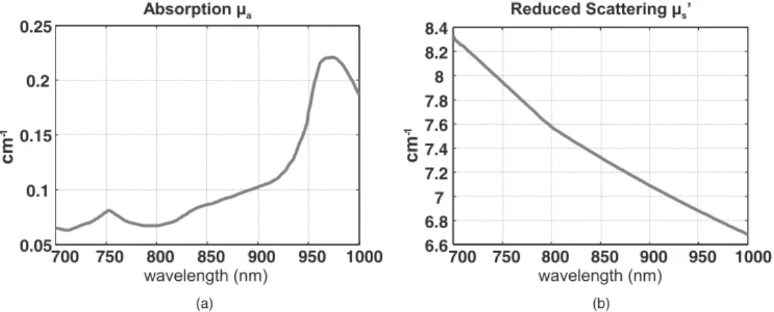
3.3 Optical Parameters

Clinical studies allowed us to have measurement of breast tissues optical parameters at our disposal. In 2001, Cerussi et al. conducted clinical measurements and obtained average re-duced scattering and absorption coefficients of breast, depend-ing on wavelength.30From those results, we defined average simulation values of absorption coefficient␮a共in inverse

cen-timeters兲 and reduced scattering coefficient ␮_s

⬘

2兲.

3.4 Light Propagation

Propagation of light in turbid media has been extensively dis-cussed. To simulate decrease of intensity emitted by fluores-cent markers embedded in diffusive tissues, and to estimate evolution of contrast between specific fluorescence and autof-luorescence depending on depth of fluorescent markers in tis-sues, classical diffusion approximation is considered. Thus, for homogeneous medium and continuous illumination, the photon density␾共in W m−2兲 satisfies the following derivative equation:

⌬␾共r兲 − k共␭兲2_{␾共r兲 = −} S共r兲

D共␭兲 共9兲

where r is the marker position in medium, the diffusion term D is defined as D = 1/共3共␮a+␮s兲兲, k is defined as k

=共3␮a␮s兲1/2, and S共r兲 is the isotropic source term. Solution␪

of this equation, assuming an infinite medium, is known. Even if the infinite medium hypothesis does not correspond to our case, it has the benefit of having an analytic solution and it

enables us to easily describe the light propagation model and changes on spectra. Such a hypothesis would be annoying for a more precise study, especially concerning side effects. For now, however, this approximation is sufficient, and the solu-tion␪ to the diffusion equation is used:

␪=exp关− k共␭兲r兴

4␲D共␭兲r . 共10兲

Wavelength-dependent absorption and reduced scattering coefficients of breast tissue are responsible for modification of markers emission spectrum. After fluorescent markers are ex-cited, the emitted photons propagate back in tissues following Eq.共9兲to finally reach detectors, as depicted in Fig.3. Thus, the emission spectrum of detected fluorescent markers Sd共␭兲

varies from ex vivo fluorescence spectrum S共␭兲:

Sd共␭兲 ⬀ S共␭兲

exp关− k共␭兲rmd兴 4␲D共␭兲rmd

, 共11兲

where r_md is the distance from fluorescent markers to detec-tors.

wavelength (nm) wavelength (nm)

Absorption µa Reduced Scattering µs’

c m -1 c m -1 700 750 800 850 900 950 1000 0.05 0.1 0.15 0.2 0.25 700 750 800 850 900 950 1000 6.6 6.8 7 7.2 7.4 7.6 7.8 8 8.2 8.4 (a) (b)

Fig. 2 Average values chosen for breast tissues共a兲 absorption and 共b兲 scattering 共inspired by Ref.30兲.

S λ D λ µa, µs’ S(λ) Sd(λ)

Fig. 3 Schemalic of light propagation after excitation by source s in

breast tissues, and detection of photons emitted back from fluorescent markers on detectors d.

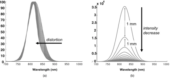
We can now simulate detected fluorescence signal, depend-ing on depth r of markers in breast tissues. Decreasdepend-ing inten-sity and spectral distortions resulting from the emitted mark-ers light travel in tissues are shown in Fig. 4 for markers moved from the surface to10 cm deep in breast tissues.

3.5 Source Number Determinacy

When running NMF on our spectroscopic data, we assume that the number of sources we are looking for is equal to the number of the different specific markers injected, plus one for the autofluorescence contribution. Distortion of fluorescence spectra could lead to an increase in the number of sources to unmix; in a case where a same marker is present at different depths in a medium, fluorescence spectrum emitted by the deepest markers appear distorted compared to the less deeply embedded markers.

When the number of sources to unmix is not empirically chosen, a method to define it is to compute the SVD of initial data M:

M = U⌺V, 共12兲

where matrix U contains spatial information of fluorescence sources, matrix V contains spectral information, and⌺ gives the ordered singular values. We thus assume our data can be expressed as a separable set of orthonormal spatial and wave-length components. By looking at the singular values, we can define number of sources in the mixed data by selecting the first nonnegligible singular values.

We ran the NMF algorithm on our simulated breast data, and give the SVD of data for each depth of markers tested, from0.1 to 10 cm. The results are presented in Fig.5. While spectrum distortion should lead us to consider a third source in our unmixing model, the exponential loss of marker signal intensity does actually not allow time for spectra to become distorted, and SVD only finds two sources.

Since spectrum distortion is insignificant in front of inten-sity loss of deep embedded markers, looking for an average spectrum S for a same family of markers, but at different depths, is sufficient in diffusive optical imaging. In last sec-tion, an in vivo unmixing example will confirm that result.

4 A Priori Information and Regularization

Many hybrid NMF algorithms, most often dealing with spar-sity and smoothness constraints, were developed in the last 5 y, most of them trying to directly adapt from Lee and Se-ung’s multiplicative update rules.31,32Kim and Park33became interested in sparse NMFs by L₁-norm constraint term mini-mization; Cichocki et al.34presented cost functions no longer based on the Kullback-Leibler divergence but on Csiszár’s ␸-divergence; while other approaches use alternative cost functions formulations.35,36 We propose in this section to study the effect of initialization of matrices A and S on NMF solutions, and we present regularized NMF update rules, adapted to spectral imaging, that deal with the a priori knowl-edge on the fluorescence spectra considered.

4.1 Influence of Initialization on NMF Decomposition

Choice of initialization is once more fundamental and NMF decomposition directly depends on the initial guess on matri-ces A and S. In that part, we study the influence of

initializa-(a) (b) 0 10 20 30 40 50 60 70 80 90 100 distortion Wavelength (nm) 0 0.5 1 1.5 2 2.5 3 3.5 x 104 1 mm 1 mm intensity decrease Wavelength (nm)

Fig. 4 Normalized fluorescence spectra of simulated markers:共a兲 spectrum distortion and 共b兲 intensity loss observed for markers moved from the surface to 10 cm deep in simulated breast tissues.

1 2 3 4 5 0 1 2 3 4 5 6 7x 10 10 1 mm 2 to 10 mm

Singular values ordering

S ing u la r va lu e

Fig. 5 From 1 mm to 10 cm in breast tissues; even if fluorescence

spectra of markers are distorted by traveling tissue, only two fluores-cence sources共markers and autofluorescence兲 are considered in the unmixing model.

tion on our simulated example. Gaussian spectra similar to simulation spectra of matrix S are chosen to initialize the NMF algorithm. We observe the influence of wavelength translation of initialization spectra on the NMF decomposi-tion. For this specific example, initialization spectra for matrix

S₀ are translated on a range of 100 nm, on both sides of simulation spectra, as depicted Fig.6.

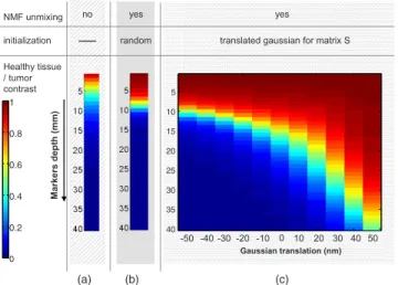
To underline the dependence of NMF result to initializa-tion, three cases are presented. For each case, resulting con-trast for different depths of fluorescent markers in tissue共from 0.1 to 4 cm兲 is obtained.

First we observe healthy tissue/tumor contrast on raw data, without any unmixing processing: contrast and detection are naturally decreasing with depth 关see Fig. 7共a兲兴. Then NMF

processing is applied on data but with random initialization 共random nonnegative values for matrices A and S, 30 draws per depth兲: unmixing processing improves detection 关see Fig.

7共b兲兴. Finally, NMF algorithm with this time Gaussian

initial-ization for S 共Gaussian models are translated in a 100-nm

range兲 is tested: even with less appropriate initialization 共in that case, when both simulation spectra are translated50 nm up that simulation models for initialization兲, contrast is im-proved compared to both prior cases关see Fig.7共c兲兴.

NMF processing without any a priori information still im-proves resulting contrast compared to results on raw data. Then, Gaussian initialization refines results.

But the initialization guess is not obvious. When the ini-tialization spectrum is translated 50 nm from the expected spectra, this initialization leads to better result than if initial-ization is equal to simulated spectra. One explanation may be that we move away from the crossing area where fluorescence spectra overlap and where indeterminacy between autofluo-rescence and fluoautofluo-rescence of markers is high. Moreover, the obtained contrast is not symmetric on both sides of the 0-shifted spectra: the fluorescence of markers is spatially re-straint compared to the autofluorescence background共see Fig.

1兲, and moving away to an initialization zone where the

fluo-rescence marker spectrum does not clash with the autofluo-rescence spectrum emission is advantageous.

From that example, we show initialization choice is very sensitive, but necessary to improve marker detection. Even if an approximate initialization already improves contrast be-tween tumor area and healthy tissue compared to the algo-rithm with random initialization共see Fig.7兲, a more accurate

initialization selection may push back the detection limits. Such selection can be obtained with a multistart initializa-tion step prior to the NMF algorithm we proposed earlier.

4.2 New Multiplicative Update Rules

As explained in previous section, a priori knowledge of fluo-rescence sources enables refining the range of solutions. By choosing appropriate initialization, detection of marked tu-mors can be improved. Another way to restrain the solutions set is to constrain the initial cost function F; we propose in this section to lightly modify the cost function, and find a new regularized algorithm to minimize updated cost function.

4.3 A Priori Knowledge on the Fluorescence

Sources

In the optical spectroscopy context, injected markers are known and could thus ease the unmixing problem. But whether it refers to the specific markers, or to the autofluores-cence of biological tissues, we can actually not define a pre-cise model of the fluorescence spectra. Spectra of the specific markers may vary from the ex vivo known spectra once in-jected in vivo and illuminated. In the in vivo medium, the markers may create new products that are able, in turn, to emit unknown fluorescence signals. Fluorescence spectra may also vary with the pH values in the medium, and their inten-sity may decline with time due to the photobleaching phe-nomenon. Even if chemical modifications appear on fluores-cent molecules under illumination or due to the receiver medium components, we usually observe after that a constant emission spectrum共except in the case of distortion of spectra due to depth of tissue, explained later兲. Finally, the optical parameters of the biological tissues—diffusion and absorption—cause emissions fluorescence spectra to vary with the depth of the fluorescent source. This last problem was treated in simulation and presented in previous section.

7000 750 800 850 900 950 1000 20 40 60 80 100 Simulated spectra Wavelength (nm) Initializations

Fig. 6 Influence of initialization on NMF decomposition is studied on

simulated example: initial spectra of matrix S0are translated

共simul-taneously for this example兲 in a range of 100 nm on both sides of expected spectra.

translated gaussian for matrix S

0 10 20 30 40 50 -10 -20 -30 -40 -50 Gaussian translation (nm) Ma rk e rs d e p th (mm ) NMF unmixing initialization random yes Healthy tissue / tumor contrast yes no (a) (b) (c) 5 10 15 20 25 30 35 40 0 0.2 0.4 0.6 0.8 1

Fig. 7 Influence of initialization on resulting contrast共breast

Regarding the autofluorescence of tissues, as for the specific markers, the illumination may be responsible for the creation of new products. Furthermore, autofluorescence spectrum may vary according to the pH of analyzed area,37or according to the patient.38–40 But once measured, the in vivo autofluo-rescence spectrum usually not differs across the organism be-ing observed. An example of mouse autofluorescence acqui-sition is given Fig. 8, where normalized spectra remain constant across the mouse body. We assume this property should also be true for specific human area observed共prostate, breast, etc.兲.

For slightly different autofluorescence emission spectra, the average spectrum is sufficient for NMF decomposition共a similar case is that for distorted fluorescent markers with depth兲.

Even if fluorescence spectra may not be initially perfectly defined, we still have some a priori information concerning them, from ex vivo and empirical measurements. The emis-sion wavelength range, and the shape of the expected spectra may be globally known and used to refine solutions set.

4.4 NMF Initialization Step

The initialization step uses a priori models to guide the solu-tions, but lets the algorithm, thanks to its blind specificity, to adapt solutions depending on the original experimental data. We would like the algorithm to take into account that piece of information: we thus define a new cost function to minimize, that directly depends on S0.

4.5 New Cost Function and Regularized Update

Rules

The new cost function F₂ is now defined as the sum of the square of the Euclidean distance between M and A⫻S plus a

regularization term on the initialization S₀, weighted by a regularization vector␣of length P:

F2=

兺

兺

冉

兺

冊

兺

兺

F2=共M − AS兲t共M − AS兲 + 共S − S0兲tD␣共S − S0兲, 共14兲 where D_␣= diag关␣₁,␣₂, . . . ,␣p兴 is a diagonal matrix

contain-ing the P regularization parameters associated to the P spectra of matrix共S−S₀兲.

The regularization term lets S vary from S0, according to the confidence we have in the initialization. Then F2is mini-mized by alternatively updating matrices A and S, with re-spect to共A,S兲艌0. We propose to use original multiplicative regularized update rules, defined as follows.

Theorem 2. The function F2 is nonincreasing under the up-date rules: S_p␭← S_p␭共A t_{M + D} ␣S0兲p␭ 共At AS + D_␣S兲p␭ A_np← Anp 共MS t_兲 np 共ASSt_兲 np , 共15兲 with D_␣= diag关␣₁,␣2, . . . ,␣p兴.

The value of␣must be set according to the level of con-fidence in the a priori information on the initial spectra. We can also use different degree of confidence on the different spectra by using a vector␣.

(a) (b) 750 800 850 900 950 0 20 40 60 80 100 Wavelength (nm) Normalized spectra autofluorescence spectra 750 800 850 900 950 0 1000 2000 3000 4000 5000 6000 7000 8000 9000 Wavelength (nm)

Autofluorescence intensity

r

Autofluorescence spectra

A

We prove Theorem 2 in the appendix, by using an auxiliary function as in Refs.11and12, and conserving the maximum of the mathematical notations of Lee and Seung in Ref.12. To illustrate the efficiency of NMF on spectroscopic data, we propose now an example on in vivo experimental data, where up to three different fluorescence sources need to be unmixed.

5 Spectral Unmixing on Experimental Data

For in vivo experiments, an autofluorescence signal is neces-sarily measured. Then several specific markers may be used to simulate marked targets, such as tumors. In this section, we test NMF to unmix three overlapping different fluorescence sources, including the autofluorescence on mice.

To acquire spectrally resolved measurements, the animal was illuminated with a planar laser at 690 nm. The emitted back fluorescence signal was collected along a line of Nx

points by a spectrometer coupled with a charge-coupled de-vice camera共Andor Technologies兲: a Nx⫻N_␭acquisition was

measured共see Fig. 9兲. For this experiment, Nx was equal to

250 and N_␭to 1024, which corresponds to a wavelength range around600 to 975 nm. A translation stage, covering Nysteps,

was then used to get a scanning of the whole animal: Ny

acquisitions were obtained, each of size Nx⫻N␭. Before to

run the NMF algorithm, mixed data of size 共Ny⫻Nx⫻N_␭兲

were reordered as a 2-D array of size 共Ny⫻Nx, N_␭兲 共Ns is

defined in NMF equation is now equal to Ny⫻Nx兲.

Sepa-rately, a black and white picture of the animal may be taken, to superimpose fluorescence signal and environment image if necessary.

For each in vivo experiment, a precise protocol is defined. All protocols have in common the following cares. The ani-mal procedure is in compliance with the guidelines of the European Union共regulation No. 86/609兲, taken in the French law 共decree 87/848兲 regulating animal experimentation. All efforts are made to minimize animal suffering. The animal manipulation is performed with sterile techniques and ap-proved by the Grenoble Animal Care and Use Committee 共France兲 共registration number 20_iRTSV Léti-FNG-02兲. An adult female nude mouse 共Janvier, Le Genest saint-isle, France兲 are used throughout the experiments. They are housed in approved facilities, at 21⫾1 °C under diurnal lighting conditions. The mice arrive at the animal facility 2 weeks before the experiments start and had free access to food and water.

5.1 Multimarker Experiment 5.1.1 Presentation

We present a first feasibility experiment on a mouse. Two glass capillary tubes respectively filled with5␮l of indocya-nine green loaded into lipid nanoparticules41 共ICG-LNP兲 at 0.35␮mol/l and 5␮l of Alexa 750 at 0.1␮mol/l were in-serted subcutaneously to simulate marked targets 关see Fig.

10共a兲兴. Three distinct fluorescent sources—autofluorescence,

ICG-LNP, and Alexa 750—whose emission spectra are over-lapping had to be unmixed. To draw a parallel between acqui-sitions with or without specific fluorescence, a first acquisition of the animal was run as a reference, without any specific markers inserted.

In this precise example, we chose␣= 1010_{to constraint the} autofluorescence spectrum to remain close to initialization Laser source

690 nm Spectrometer

Translation stage: Nysteps

anesthezia B&W camera Nλ Nx 8009001000 50 8009001000 50 1002003004005006007008009001000 50 100 150 200 250 Ny CCD camera Nx

Fig. 9 Experimental setup for acquisition of the animal and data

processing. Anesthetized mouse ICG-LNP Capillary tube (a) (b) (c) (d) Alexa 750 Small incision Anatomy _Acquisitions No capillary tube (Autofluorescence) ICG-LNP Alexa 750

ICG-LNP + Alexa 750 tubes

(Autofluorescence + ICG-LNP + Alexa 750) T1 T2 N C_{T2 ,N}= 0.3631 C_{T1 ,N}= 0.2123

Fig. 10 共a兲 Schematic of the mouse with two capillary tubes filled with ICG-LNP and Alexa 750; 共b兲 anatomy scheme of the mouse, 共c兲 scanning result without any capillary共autofluorescence signal only兲, and 共d兲 scanning result with the two capillary tubes inserted 共autofluorescence + ICG-LNP + Alexa 750兲.

and have a plausible profile, and␣= 0 for ICG-LNP, and Al-exa 750 spectra. The regularization term helped to smooth over aberrations due to the two components crosstalk on re-sulting spectra. We chose initialization from empirical results, but could not use multistart initialization: regularization on initialization asks for coherent initialization spectra, while multistart initialization may use translated spectra uncon-nected to real expected fluorescence spectra. The choice has to be made between different regularization methods, depend-ing on application.

5.1.2 Results

Figure 10共c兲 shows the reference acquisition of the mouse without any capillary: the autofluorescence is the only fluo-rescence signal measured. Autofluorescent areas may be at-tributed to some specific organs, known to emit natural fluo-rescence, such as the stomach, the liver, the intestine, or the kidneys of the animal, if we compare the autofluorescence scanning to the anatomy scheme of a mouse关Fig.10共b兲兴. In

the same figure, we present the resulting scanning of the mouse with the two capillary tubes of ICG-LNP and Alexa 750关Fig.10共d兲兴, on which the regularized NMF algorithm is

run.

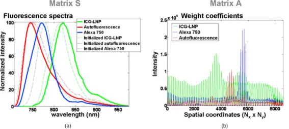
Figure11presents the overlapping spectra that NMF suc-cessfully unmixed. The three normalized spectra of matrix S presented in Fig.11共a兲are weighted by coefficients of matrix

A 关Fig. 11共b兲兴. The three resulting contributions of

fluores-cence are presented in Fig. 12: the autofluorescence 关Fig.

12共a兲兴, the ICG-LNP 关Fig. 12共b兲兴, and the Alexa 750 关Fig. 12共c兲兴. Three sources unmixing allowed improving detection

for each marker, Alexa 750 and ICG LNP. Indeed, initial con-trast values 共measured on mixed data, cf. Fig. 10 between markers area and normal tissue area were equal to 0.2123 for ICG-LNP and 0.3631 for Alexa 750兲. After unmixing, contrast values respectively reached 0.6366 共ICG-LNP兲 and 0.6763 共Alexa 750兲 共see Figs.12共b兲and12共c兲兴.

To conclude concerning this feasibility experiment, a last comparison is made, between the original autofluorescence scanning 共without any capillary tube inserted to the animal兲 and the separated autofluorescence results obtained for both past experiments 共see Fig. 13兲. First, a consistent intensity

level is obtained after the NMF decomposition. Indeed, the intensity obtained after NMF decomposition for the autofluo-rescence part关Fig.13共b兲兴 is close to the intensity observed on

the reference autofluorescence acquisition 关Fig. 13共a兲兴.

Fi-nally, the principal autofluorescent area observed on the au-tofluorescence scanning关Fig.13共a兲兴 are also present on

autof-luorescence contribution obtained after the NMF decomposition关Fig.13共b兲兴.

5.2 Multidepth Experiment

In a second experiment, we proposed to test the NMF algo-rithm robustness on a precise case of the same fluorescent marker at two different depths in mouse tissues. In such a case, the deeper the markers are embedded in tissues, the more their fluorescence spectra are distorted and their inten-sity is exponentially decreased.

Two glass capillary tubes both filled with 5␮l of ICG-LNP共Ref.41兲 at 5␮mol/l were inserted to simulate marked targets. The first tube was inserted subcutaneously 共around 1 mm deep兲, while the second one was placed in the rectum of the animal 共around 6 mm deep from the surface兲, as de-picted in Fig.14共a兲. The same experimental setup was used to scan the mouse 共see Fig. 9兲, and the obtained data are

pre-sented Fig.14共b兲. The6-mm-deep marker signal was mixed with the autofluorescence signal and masked by the

1-mm-deep intense marker signal, and the

5 mm-deep-difference was responsible for light distortion 共emission peak translation兲 and loss of intensity between both emitted spectra, measured in the rectum or subcutaneously 关see Fig.14共b兲兴.

5.2.1 Results

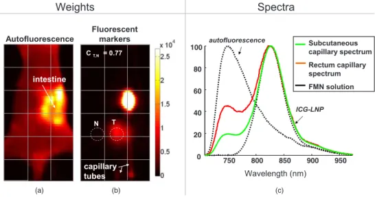
As for the previous experiment, we ran the NMF algorithm on the mixed data to obtain separated fluorescence contributions of autofluorescence and the specific ICG-LNP fluorescence. The results are presented Fig.15, with a unique average spec-trum obtained in matrix S after NMF decomposition for the ICG-LNP despite the slightly different spectra emitted from the subcutaneous and rectum capillaries 共see Fig. 15, ICG-LNP dotted line兲, and accurate unmixing results were

ob-(a) (b)

Fig. 11 Results after NMF:共a兲 fluorescence spectra obtained 共matrix S兲: initialization 共dotted lines兲, and results of the NMF decomposition 共continuous lines兲, and 共b兲 weight coefficients 共matrix A兲.

tained 关see Figs. 15共a兲 and 15共b兲兴. Deep markers that were

originally mixed with autofluorescence signal are now easily detectable. Indeed, after autofluorescence removal, detection of6-mm-deep markers was considerably improved. The ini-tial contrast value between the ICG-LNP rectum area and the normal tissue area was equal to 0.36 before unmixing 关see Fig.14共b兲兴, and reached 0.77 once the fluorescence

contribu-tions were separated 关see Fig. 15共b兲兴. Moreover, in the

ob-tained ICG-LNP contribution, all the autofluorescence critical zones共the stomach or intestine, for example兲 were quenched.

6 Conclusions

We presented a blind positive source separation method ap-plied to in vivo spectrally resolved data. Beyond the specific fluorescence signal of specific markers used in optical imag-ing, the autofluorescence of biological tissues was also de-tected in the wavelength range we used, and must be removed to achieve accurate detection results. This property increased with the depth of biological tissues explored, since the spe-cific signal decreases exponentially while the autofluores-cence signal remains constant. To remove autofluoresautofluores-cence and unmix different fluorescent markers whose fluorescence

spectra are not perfectly known, a blind source separation method, the NMF, was chosen. By notably taking into account the nonnegativity of the data, it is particularly suitable for fluorescence imaging data. We briefly presented this classical method, from the choice of the cost function and the optimi-zation step that minimizes it and leads to a nonunique NMF decomposition. Indeed, when using blind source separation, we estimated fluorescence sources without knowing the mix-ing process; without some a priori knowledge, it is not pos-sible to uniquely estimate the sources. We presented studies of simulated breast data that underline interest of a priori infor-mation for initialization choice and additional constraints that may be applied to cost functions. An original regularized NMF algorithm that takes into account some prior knowledge about the fluorescence spectra was proposed. We did not dis-cuss a method to chose the value of the regularization param-eter, which is currently empirically chosen. Finally, our theory was successfully validated with in vivo experiments on mice. The aim of those experiments was to remove the autofluores-cence contribution from the experimental data, and to unmix upto two specific markers, or the same fluorescent marker at different depths in tissues. NMF computed satisfactory results and enabled us to localize specific marker contributions ini-tially lost in the autofluorescence signal.

As optical imaging tries to detect deeper and deeper em-bedded targets, NMF is a useful preprocessing step to remove unwanted autofluorescence and unmix different spectra of in-terest. By returning separated fluorescence contribution data, the method presents the possibility to perform accurate to-mographic reconstructions and thus to confirm the 3-D posi-tion of marked tumors.

Appendix: Theorem 1: Proofs of Convergence

In this section, we propose a proof of convergence of Theo-rem 2. Note that a proof for convergence of the update rule for

A was already given by Lee and Seung.12We introduce the following definition: (a) (b) (c) ICG-LNP Autofluorescence Alexa 750 CT,N = 0.6763 T N _N T CT,N = 0.6366

Fig. 12 Results after NMF:共a兲 autofluorescence intensity contribution, 共b兲 ICG-LNP intensity contribution, and 共c兲 Alexa 750 intensity contribution. Original autofluorescence measurement Autofluorescence after NMF (a) (b)

Fig. 13 共a兲 Autofluorescence measurement, without any specific fluo-rescence共no capillary tubes兲 added and 共b兲 autofluorescence contri-bution obtained after NMF decomposition 共two capillary tubes of ICG-LNP and Alexa 750 experiment兲.

Anesthezia (isofluorane) Rectum capillary (6 mm deep) Subcutaneous capillary (1 mm deep) Mixed data Acquisition Experiment Supine position (a) (b) 750 800 850 900 950 Wavelength (nm) subcutaneous rectum T N CT,N = 0.36

Fig. 14 共a兲 Two capillary tubes of ICG-LNP are placed at two different depths and共b兲 intensity data obtained and average fluorescence spec-tra measured in the capillary tubes.

Definition 1. G共s,si_{兲 is an auxiliary function for F}

2共s兲 if the following conditions are satisfied:

G共s,si兲 艌 F2共s兲 and G共s,s兲 = F2共s兲. 共16兲 The auxiliary function definition is useful for the following lemma:12

Lemma 1. If G is an auxiliary function for F2, then F2 is nonincreasing under the update:

si+1= argminsG共s,si兲 共17兲

Lemma 1 is illustrated in Fig.16.

By defining an appropriate auxiliary function G for F2, as defined earlier, the update rules presented in Theorem 1 sim-ply follow from Lemma 1关Eq.共17兲兴. The auxiliary function G is presented in the following lemma.

Lemma 2. If K共si_{兲 is the diagonal matrix}

Kab共si兲 = ␦ab共AtAsi+␣⫻ si兲a s_ai , 共18兲 then, setting⌬s=共s−si_兲, G共s,si兲 = F2共si兲 + ⌬stⵜ F2共si兲 + 1 2⌬s t_K共si_{兲⌬s, 共19兲}

is an auxiliary function for

F2共s兲 = 1 2

兺

冉

兺

冊

兺

Proof of lemma 2. G共s,si_{兲 is an auxiliary function for F}

2共s兲 if the conditions defined in Eq. 共16兲 are verified. If G共s,s兲 = F2共s兲 is obvious, the second condition G共s,si兲艌F2共s兲 must be demonstrated.

LetⵜF₂ be the gradient of F₂and Hess共F₂兲 the Hessian matrix. We obtain F2共s兲 = F2共si兲 + ⌬stⵜ F2共si兲 + 1 2⌬s t_Hess共F 2兲⌬s, 共21兲 with F2共si兲 = 1 2储m − As i_储2₊␣ 2储s i_{− s} 0 i_储2₌1 2共m − As i_兲t_{共m − As}i_兲 +␣ 2共s i_{− s} 0 i_兲t_共si_{− s} 0 i_{兲, 共22兲}

and finally the gradient is

ⵜF2共si兲 = At共Asi− m兲 +␣共si− s0

i_{兲, 共23兲}

while the Hessian matrix gives

Fluorescent markers Autofluorescence Weights Subcutaneous capillary spectrum Rectum capillary spectrum FMN solution intestine capillary tubes Spectra (a) (b) (c) Wavelength (nm) 750 800 850 900 950 0 20 40 60 80 100 ICG-LNP autofluorescence T N CT,N = 0.77

Fig. 15 Unmixing results:共a兲 and 共b兲 weights 共matrix A兲 of respectively autofluorescence and ICG-LNP fluorescence, and 共c兲 unmixed spectra

共matrix S兲 obtained at convergence, and a comparison with unmixed spectra measured in capillary tubes on the mouse, subcutaneously and in the rectum.

s

s

s

G(s,s

₎

F

(s)

Fig. 16 Minimizing the auxiliary function G共s,si_兲艌F

2共s兲 ensures that

Hess共F2兲 = AtA + aIp, 共24兲 where I is the p⫻p identity matrix.

Thus, G共s,si兲 − F2共s兲 = F2共si兲 + ⌬stⵜ F2共si兲 + 1 2⌬s t_K共si_{兲⌬s − F} 2共si兲 −⌬stⵜ F2共si兲 − 1 2⌬s t_Hess共F 2兲⌬s =1 2⌬s t_关K共si_{兲 − Hess共F} 2兲兴⌬s = 1 2⌬s t_共K共si_兲 − At_{A −␣I兲⌬s. 共25兲}

Hence, the following equivalence is given

G共s,si_{兲 艌 F}

2共s兲 ⇔ ⌬st关K共si兲 − AtA −␣I兴⌬s 艌 0. 共26兲 We can now demonstrate that ⌬st_关K共si_兲−At_{A −␣I兴⌬s is}

positive: ⌬st_关K共si_{兲 − A}t_{A −␣I兴⌬s} =

兺

兺

冋

册

兺

兺

再

冋

兺

兺

册

冎

兺

冉

兺

冊

兺

冉

冊

兺

冉

冊

兺

冋

冉

冊

冉

冊

册

Following is a demonstration of Theorem 1.

Proof of theorem 1. Lemma 1 gives si+1_{= argmin}

sG共s,si兲. Since ∀a,␦G共s,si兲 ␦s_ai =关ⵜF2共s兲兴a+关K共s兲⌬s兴a= 0⇒ ⌬s = − K共s兲−1ⵜ F2共s兲, 共28兲 we obtain ∀a,sa i+1 − s_ai = −

兺

1. V. Ntziachristos, “Visualization of antitumor treatment by means of fluorescence molecular tomography with an annexin v-cy5.5 conju-gate,”Proc. Natl. Acad. Sci. U.S.A.101共33兲, 12294–9 共2004兲.

2. J. Hung, S. Lam, J. Leriche, and B. Palcic, “Autofluorescence of normal and malignant bronchial tissue,”Lasers Surg. Med. 11共2兲,

99–105共1991兲.

3. D. Wood, G. Feke, D. Vizard, and R. Papineni, “Refining epifluores-cence imaging and analysis with automated multiple-band flat-field correction,” Nat. Methods 5, i–ii共2008兲.

4. C. Vandelest, E. Versteeg, J. Veerkamp, and T. Vankuppevelt, “Elimi-nation of autofluorescence in immunofluorescence microscopy with digital image processing,” J. Histochem. Cytochem. 43共7兲, 727–730 共1995兲.

5. R. Levenson and P. Cronin, “Spectral imaging of deep tissue,” U.S. Patent No. 7,321,791共2008兲.

6. C. Hoyt, “Systems and methods for in vivo optical imaging and mea-surement,” U.S. Patent No. 7,477,931共2009兲.

7. P. Cronin and P. J. Miller, “Spectral imaging,” U.S. Patent No. 6,930,773共2005兲.

8. L. De Lathauwer, B. De Moor, and J. Vandewalle, “Blind source separation by higher-order singular value decomposition,” Proc. Eur.

Signal Processing Conf. (EUSIPCO), Vol. 1, pp. 175–178共1994兲.

9. R. C. Henry, “Current factor analysis receptor models are ill-posed,”

Atmos. Environ.21共8兲, 1815–1820 共1987兲.

10. P. Paatero and U. Tapper, “Positive matrix factorization: a non-negative factor model with optimal utilization of error estimates of data values,”Environmetrics5共2兲, 111–126 共1994兲.

11. A. Dempster, N. Laird, and D. Rubin, “Maximum likelihood from incomplete data via the EM algorithm,” J. R. Stat. Soc. 39共1兲, 1–38 共1977兲.

12. D. Lee and H. Seung, “Algorithms for non-negative matrix factoriza-tion,” Adv. Neural Inf. Process. Syst. 13, 556–562共2001兲.

13. W. Lawton and E. Sylvestre, “Self modeling curve resolution,” Tech-nometrics13共3兲, 617–633 共1971兲.

14. A. Pascual-Montano, P. Carmona-Saez, M. Chagoyen, F. Tirado, J. M. Carazo, and R. D. Pascual-Marqui, “bionmf: a versatile tool for non-negative matrix factorization in biology,” BMC Bioinf. 7共1兲,

366–375共2006兲.

15. A. Cichocki and A. H. Phan, “Fast local algorithms for large scale nonnegative matrix and tensor factorizations,”IEICE Trans. Funda-mentalsE92A共3兲, 708–721 共2009兲.

16. V. Pauca, F. Shahnaz, M. Berry, and R. Plemmons, “Text mining using nonnegative matrix factorizations,” in Proc. 4th SIAM Int.

Conf. on Data Mining, pp. 452–456共2004兲.

17. H. Xu, C. Kuo, and B. W. Rice, “Improved sensitivity by applying spectral unmixing prior to fluorescent tomography,” in Proc. OSA

Biomed. Opt., paper BMC1共2008兲.

18. C. Gobinet, E. Perrin, and R. Huez, “Application of nonnegative matrix factorization to fluorescence spectroscopy,” in Proc. Eur.

Sig-nal Processing Conf. (EUSIPCO), pp. 6–10共2004兲.

19. C. Gobinet, V. Vrabie, A. Tfayli, O. Piot, R. Huez, and M. Manfait, “Preprocessing and source separation methods for Raman spectra analysis of biomedical samples,” in Proc. EMBS 29th Annu. Int.

Conf. of the IEEE, pp. 6207–6210共2007兲.

20. H. Xu and B. W. Rice, “In vivo fluorescence imaging with a multi-variate curve resolution spectral unmixing technique,” J. Biomed. Opt.14共6兲, 064011 共2009兲.

21. P. Paatero, “Least squares formulation of robust non-negative factor analysis,”Chemom. Intell. Lab. Syst.37共1兲, 23–35 共1997兲.

22. W. H. Press, S. A. Teukolsky, W. T. Vetterling, and B. P. Flannery,

Numerical Recipes: The Art of Scientific Computing, Cambridge

Uni-versity Press, New York共2007兲.

23. S. Moussaoui, D. Brie, and J. Idier, “Non-negative source separation: range of admissible solutions and conditions for the uniqueness of the solution,” in Proc. IEEE Int. Conf. on Acoustics, Speech, and Signal

Processing, Vol. 5, pp. 289–292共2005兲.

24. A. Cichocki, S. Amari, A.-H. Phan, and R. Zdunek, Nonnegative

Matrix and Tensor Factorizations: Applications to Exploratory Multi-way Data Analysis and Blind Source Separation, Wiley-Blackwell,

Chichester, UK共2009兲.

25. Z. Jin, V. Josserand, S. Foillard, D. Boturyn, P. Dumy, M. Favrot, and J. Coll, “In vivo optical imaging of integrin alphaV-beta3 in mice using multivalent or monovalent cRGD targeting vectors,” Molec.

Cancer 41, 1–9共2007兲.

26. Y. Urano, D. Asanuma, Y. Hama, Y. Koyama, T. Barrett, M. Kamiya, T. Nagano, T. Watanabe, A. Asegawa, and P. Choyke, “Selective molecular imaging of viable cancer cells with pH-activatable fluores-cence probes,”Nat. Med.15, 104–109共2008兲.

27. R. Weissleder, C. Tung, U. Mahmood, and A. Bogdanov, “In vivo imaging of tumors with protease-activated near-infrared fluorescent probes,”Nat. Biotechnol.17, 375–378共1999兲.

28. J. Razkin, V. Josserand, D. Boturyn, Z. Jin, P. Dumy, M. Favrot, J. Coll, and I. Texier, “Activatable fluorescent probes for tumour-targeting imaging in live mice,” ChemMedChem 1, 1069–1072

共2006兲.

29. Z. Jin, J. Razkin, V. Josserand, D. Boturyn, A. Grichine, I. Texier, M. Favrot, P. Dumy, and J. Coll, “In vivo noninvasive optical imaging of receptor-mediated RGD internalization using self-quenched Cy5-labeled RAFT-c共-RGDfK-兲 共4兲,” Mol. Imaging 6, 43–55 共2007兲. 30. A. Cerussi, A. Berger, F. Bevilacqua, N. Shah, D. Jakubowski, J.

Butler, R. Holcombe, and B. Tromberg, “Sources of absorption and scattering contrast for near-infrared optical mammography,”Acad. Radiol.8, 211–218共2001兲.

31. A. Cichocki, R. Zdunek, and S. Amari, “New algorithms for non-negative matrix factorization in applications to blind source

separa-tion,” in Proc. IEEE Int. Conf. on Acoustics, Speech and Signal

Pro-cessing, Vol. 5共2006兲.

32. M. Berry, M. Browne, A. Langville, V. Pauca, and R. Plemmons, “Algorithms and applications for approximate nonnegative matrix factorization,”Comput. Stat. Data Anal.52共1兲, 155–173 共2007兲.

33. H. Kim and H. Park, “Non-negative matrix factorization based on alternating non-negativity constrained least squares and active set method,”SIAM J. Matrix Anal. Appl.30共2兲, 713–730 共2008兲.

34. A. Cichocki, R. Zdunek, and S. Amari, “Csiszar’s divergences for non-negative matrix factorization: family of new algorithms,”Lect. Notes Comput. Sci.3889, 32–39共2006兲.

35. A. Hamza and D. Brady, “Reconstruction of reflectance spectra using robust nonnegative matrix factorization,”IEEE Trans. Signal Pro-cess.54共9兲, 3637–3642 共2006兲.

36. I. Dhillon and S. Sra, “Generalized nonnegative matrix approxima-tions with Bregman divergences,” Adv. Neural Inf. Process. Syst. 18, 283–290共2006兲.

37. P. Juzenas, V. Iani, S. Bagdonas, R. Rotomskis, and J. Moan, “Fluo-rescence spectroscopy of normal mouse skin exposed to 5-aminolaevulinic acid and red light,”J. Photochem. Photobiol., B

61共1–2兲, 78–86 共2001兲.

38. D. C. G. de Veld, M. Skurichina, M. J. H. Witjes, R. P. W. Duin, D. J. C. M. Sterenborg, W. M. Star, and J. L. N. Roodenburg, “Autof-luorescence characteristics of healthy oral mucosa at different ana-tomical sites,”Lasers Surg. Med.32, 367–376共2003兲.

39. G. Weagle, P. E. Paterson, J. Kennedy, and R. Pottier, “The nature of the chromophore responsible for naturally occurring fluorescence in mouse skin,”J. Photochem. Photobiol., B2, 313–320共1988兲.

40. K. Onizawa, N. Okamura, H. Saginoya, J. Yusa, T. Yanagawa, and H. Yoshida, “Fluorescence photography as a diagnostic method for oral cancer,”Oral Oncol.38, 343–348共2002兲.

41. F. P. Navarro, M. Berger, M. Goutayer, S. Guillermet, V. Josserand, P. Rizo, F. Vinet, and I. Texier, “A novel indocyanine green nanoparticle probe for noninvasive fluorescence imaging in vivo,” Progr. Biomed.