HAL Id: hal-01896092
https://hal.archives-ouvertes.fr/hal-01896092
Submitted on 16 Oct 2018
HAL is a multi-disciplinary open access
archive for the deposit and dissemination of
sci-entific research documents, whether they are
pub-lished or not. The documents may come from
teaching and research institutions in France or
abroad, or from public or private research centers.
L’archive ouverte pluridisciplinaire HAL, est
destinée au dépôt et à la diffusion de documents
scientifiques de niveau recherche, publiés ou non,
émanant des établissements d’enseignement et de
recherche français ou étrangers, des laboratoires
publics ou privés.
Anderson model out of equilibrium: Decoherence effects
in transport through a quantum dot
Raphaël van Roermund, Shiue-Yuan Shiau, M. Lavagna
To cite this version:
Raphaël van Roermund, Shiue-Yuan Shiau, M. Lavagna. Anderson model out of equilibrium:
Deco-herence effects in transport through a quantum dot. Physical Review B: Condensed Matter and
Ma-terials Physics (1998-2015), American Physical Society, 2010, 81 (16), �10.1103/PhysRevB.81.165115�.
�hal-01896092�
Anderson model out of equilibrium: Decoherence effects in transport through a quantum dot
Raphaël Van Roermund, Shiue-yuan Shiau, and Mireille Lavagna
*
Commissariat à l’Energie Atomique de Grenoble, INAC/SPSMS, 17 rue des Martyrs, 38054 Grenoble Cedex 9, France 共Received 11 January 2010; revised manuscript received 18 March 2010; published 26 April 2010兲
The paper deals with the nonequilibrium two-lead Anderson model, considered as an adequate description for transport through a dc biased quantum dot. Using a self-consistent equation-of-motion method generalized out of equilibrium, we calculate a fourth-order decoherence rate ␥共4兲 induced by a bias voltage V. This decoherence rate provides a cutoff to the infrared divergences of the self-energy showing up in the Kondo regime. At low temperature, the Kondo peak in the density of states is split into two peaks pinned at the chemical potential of the two leads. The height of these peaks is controlled by␥共4兲. The voltage dependence of the differential conductance exhibits a zero-bias peak followed by a broad Coulomb peak at large V, reflecting charge fluctuations inside the dot. The low-bias differential conductance is found to be a universal function of the normalized bias voltage V/TK, where TKis the Kondo temperature of the model, which has been improved in comparison with previous approaches. The universal scaling with a single energy scale TK at low-bias voltages is also observed for the renormalized decoherence rate␥共4兲/TK. We discuss the effect of␥共4兲on the crossover from strong- to weak-coupling regime when either the temperature or the bias voltage is increased.
DOI:10.1103/PhysRevB.81.165115 PACS number共s兲: 72.15.Qm, 73.23.Hk, 75.20.Hr
I. INTRODUCTION
Over the last 10 years, an intense experimental and theo-retical activities have been developed to study quantum dots. Due to the presence of strong electronic correlations in the dot, these mesoscopic systems give rise to rich collective phenomena such as the Coulomb blockade 共CB兲 and the Kondo effect. Their manifestations in transport can be stud-ied in a detailed and controlled way in such devices as semiconductor-based quantum dots embedded in a two-dimensional electron gas1 or carbon nanotubes.2 One of the great interests of these systems is to offer the possibility of studying them under nonequilibrium conditions when either a bias voltage is applied to the leads or an electromagnetic field irradiates the device.
A simple model describing quantum dots is the Anderson model3 in which the dot is represented by a localized level
connected to Fermi seas of conduction electrons through tun-neling barriers. When the dot is singly occupied, it has been shown that the linear conductance increases as one lowers the temperature and eventually reaches the unitary limit 2e2/h in the case of symmetric coupling to the leads. This was predicted in the context of quantum dots 20 years ago4,5
and was observed experimentally about 10 years later.1,2
While in equilibrium most of the properties of the Kondo effect are now well understood6thanks to the development of
a panel of powerful techniques 关e.g., renormalization group, Bethe ansatz, Fermi-liquid theory, conformal field theory, density-matrix renormalization group, slave boson, and equation-of-motion 共EOM兲 approaches兴, most of these tech-niques fail out of equilibrium. Hence there is a huge interest to develop new techniques to tackle the problem of the Kondo effect out of equilibrium and more generally nonequi-librium effects in strongly correlated electron systems.
Theoretically, the Kondo effect out of equilibrium has been investigated by a variety of techniques developed most of the time within the Keldysh formalism: perturbation-theory and perturbative renormalization-group
approaches,7–12 slave-boson formulation solved by using
ei-ther mean-field13 or noncrossing approximation,14 and
equation-of-motion approaches.15,16 Exact solutions at the Toulouse limit have been proposed.17 Other ones have
ex-tended the Bethe ansatz out of equilibrium18,19 and in some cases have used the results to construct a Landauer-type pic-ture of transport through the quantum dot. There have also been important efforts to develop numerical techniques such as time-dependent numerical renormalization group 共NRG兲,20,21 time-dependent density-matrix renormalization
group,22and imaginary-time theory solved by using quantum
Monte Carlo 共QMC兲.23 All those approaches have only a
limited validity of their parameter regimes since they mostly describe the properties of the system in its ground state and not in its excited many-body states reached when the bias voltage drives a current through the dot.
At equilibrium, when the dot is singly occupied and pos-sesses a degenerate ground state, a Kondo effect takes place associated with a resonant spin-flip scattering of the lead electrons off the dot at the Fermi energy. In perturbation theory with respect to the Kondo coupling, it corresponds to an infrared logarithmic divergence of the conduction-electron T matrix. A finite temperature, magnetic field or bias voltage would destroy the resonant spin-flip scattering by cutting off the logarithmic divergence. Even if the smearing occurs by different ways in each of these three cases, all of them introduce a finite decoherence rate ␥. In the case of a bias voltage, the decoherence is due to the current driven through the dot. The goal of the paper is to study the deco-herence effects induced by bias voltage in detail.
In this paper, we develop an EOM approach to tackle the nonequilibrium Kondo effect in quantum dots and study the decoherence effects induced by a bias voltage. The EOM method, though conceptually simple, requires some care. The recursive application of the Heisenberg equation of motion24
generates an infinite hierarchy of equations, which relate the different Green’s functions of the system. This hierarchy has to be truncated by a suitable approximation scheme in order to form a closed set of equations. The choice of the trunca-1098-0121/2010/81共16兲/165115共19兲 165115-1 ©2010 The American Physical Society
tion scheme is crucial in order to treat carefully the correla-tion effects both from the Coulomb interaccorrela-tion and from the dot-lead tunneling.
The EOM technique was applied to the original Anderson model at equilibrium a long time ago25–27 in the context of
the dilute magnetic alloys. When applying the standard ap-proximation based on a truncation of the equations of motion at second order in the hybridization term t, it yields results which agree with perturbation-theory calculations for tem-peratures above the Kondo temperature, TK. This truncation
scheme is usually referred to as the Lacroix approximation.27,28 Even though the scheme has serious drawbacks at this level of approximation共underestimation of the Kondo temperature TK, absence of Kondo effect just at
the particle-hole symmetric point兲, it is acknowledged to pro-vide a valuable basis for the description of the Kondo effect both at high and low temperatures. The applicability of the Lacroix approximation is nicely reported in a recent paper by Kashcheyevs et al.29
In early 1990s, Meir et al.30undertook to apply the EOM
method to the study of quantum dots out of equilibrium and/or in the presence of a magnetic field. They used a sim-plified version of the Lacroix approximation, which fails to account for the finite decoherence rates induced by bias volt-age and/or magnetic field. Meir et al. proposed to introduce them heuristically by making use of the Fermi golden rule. They obtained interesting results for the bias voltage depen-dence of the differential conductance showing a zero-bias anomaly but the weakness of the approach is that it does not constitute an unified and consistent frame for the treatment of the Kondo effect in the presence of the decoherence ef-fects induced out of equilibrium.
There have been recent attempts to use an approximation which truncates the equations of motion at higher order in t.15,16,31 Their authors claimed to improve quantitatively at
equilibrium the Kondo temperature and the density of states around the Fermi energy and have been able to investigate some nonequilibrium issues. However, there is need to clarify the decoherence effects in the framework of the EOM method.
The organization of the paper is the following: in Sec.II, we outline the EOM formalism and the main steps of the proposed approximation based on a truncation of the equa-tions of motion at the fourth order in t. An analytical ex-pression of the retarded Green’s function in the dot is derived involving expectation values which are determined self-consistently. The details of the calculations are presented in Appendices A and B.
An analytical study of this Green’s function is presented in Sec. III. Namely, we deduce the renormalization effects and the decay rates involved at the second order in tfor the different regimes of the Anderson model. Special care is given to the singly occupied dot regime, for which the van-ishing of one of the decay rates leads to the low-energy loga-rithmic divergence of the self-energy of the dot Green’s func-tion, yielding a Kondo resonance peak in the density of states. We show how the approximation scheme allows one to derive a decoherence rate out of equilibrium which be-comes finite as soon as a bias voltage is applied. This deco-herence rate provides a cutoff to the logarithmic divergence
present at equilibrium in the Kondo regime. We show how our approximation scheme improves the result for the Kondo temperature TK upon earlier predictions.
We present in Sec. IV our numerical results—both at equilibrium and out of equilibrium—for the density of states, the 共linear and differential兲 conductance, and the bias-induced decoherence rate. A self-consistent treatment is re-quired in order to determine the expectation values involved in the Green’s function of the dot. At equilibrium, the density of states in the particle-hole symmetric case shows a three-peak structure at low temperature with a Kondo resonance peak in the local-moment regime. This result constitutes an advantage of our approximation scheme compared to the La-croix approximation. The unitary limit for the linear conduc-tance G = 2e2/h is analytically recovered at zero temperature
in the particle-hole symmetric case when the dot is sym-metrically coupled to the leads. Numerically, one notices a slight underestimation of G due to the numerical accuracy of the self-consistent treatment.
Out of equilibrium, the spectral function shows a splitting of the Kondo peak into two peaks pinned at the chemical potentials of the two leads. The height of the peaks dimin-ishes when the bias voltage increases, meaning that the Kondo effect is destroyed by decoherence induced out of equilibrium. This influences the evolution of the differential conductance as a function of bias voltage, which shows a zero-bias anomaly followed by a broad Coulomb peak. At low-bias voltage, we check that the differential conductance follows a universal scaling law which depends on a single energy scale, TK. Comparison is made with results obtained
by recent numerical techniques for nonequilibrium such as time-dependent NRG 共Ref. 21兲 and imaginary-time theory
solved by QMC.23,32
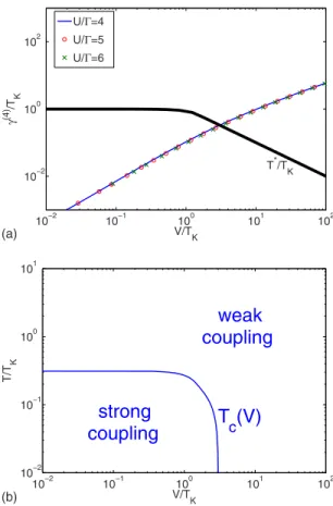
Finally, we compute the bias voltage dependence of the decoherence rate and discuss the crossover from strong-coupling to weak-strong-coupling regime depending on the com-parison between the decoherence rate and a characteristic energy scale Tⴱ. We show the existence of a crossover be-tween the strong-coupling and weak-coupling regimes when either the temperature or the bias voltage is raised, as pre-dicted by other methods.
II. EQUATION-OF-MOTION FORMALISM
We model the quantum dot connected to the two leads by the single-level共spin-1/2兲 Anderson impurity Hamiltonian,
H = Hlead+ Hdot+ Hint, 共1兲
Hlead=
兺
␣k␣k c␣k† c␣k, Hdot=兺
n+ Un↑n↓, Hint=兺
␣k共t␣ c␣k† f+ H.c.兲,where c␣k† 共c␣k兲 is the creation 共annihilation兲 operator of an electron of momentum k and spin 共=⫾1兲 in the␣共=L,R兲
lead共with energy ␣k=k−␣兲;␣is the chemical potential
in the␣lead; f†共f兲 is the creation 共annihilation兲 operator of an electron of spin in the quantum dot 共with energy =d+B/2 when the Zeeman splitting B is included兲; n
= f†f is the number operator for electrons of spin in the dot; U is the Coulomb interaction between two electrons of opposite spin in the dot; and t␣ is the tunneling matrix ele-ment between the state兩k典 in the␣lead, and the state兩典 in the dot. For simplicity, we assume t␣to be real and k inde-pendent.
When a bias voltage is applied to the leads 共eV=L
−R兲, the system is driven out of equilibrium and a current is
induced through the quantum dot. The current I for the Anderson model is expressed by the generalized Landauer formula33accounting for the interactions among electrons
I =2e ប
兺
冕
−W W d ⌫L共兲⌫R共兲 ⌫L共兲 + ⌫R共兲 关fF L共兲 − f F R共兲兴 共兲, 共2兲 where W is the half bandwidth of the conduction-electron band in the leads,⌫␣共兲 is the tunneling rate of the spin dot electron at energy into the lead ␣, defined as ⌫␣共兲 =兺kt␣2 ␦共−␣k兲=t␣2 ␣0共兲 with ␣0共兲 theunrenormal-ized density of states at energy in the lead ␣, fF␣共兲
=兵exp关共−␣兲兴+1其−1 is the Fermi-Dirac distribution
func-tion in the␣lead,共兲, the local density of states for spin in the dot, can be expressed in terms of the retarded electron Green’s function in the dot Gr共兲 according to 共兲 = −1/ImGr共兲.
As pointed out in Ref.33, Eq.共2兲 is valid provided that
the tunneling couplings for both leads ⌫L共兲 and ⌫R共兲
differ only by a constant multiplicative factor. The task is to compute the retarded electron Green’s function in the dot defined as Gr共兲=−i兰0⬁dteit具兵f共t兲, f†共0兲其典, where =+ i␦ 共␦→0+兲. In order to simplify the notations in the rest of the
paper, the imaginary part i␦ going alongside will be im-plicit while the summation over k implies summation over both␣and k. Hence we write in a shorthand notation
兺
␣=L,R
兺
kt␣→
兺
k
t.
Using the Zubarev notation24 for the retarded Green’s
func-tions involving fermionic operators A and B 具具A,B典典 = − i lim
␦→0+
冕
0⬁
dtei共+i␦兲t具兵A共t兲,B共0兲其典, 共3兲
which can be integrated by parts and using the Heisenberg equation of motion, one can show the following relation:
具具A,B典典 = 具兵A,B其典 + 具具关A,H兴,B典典. 共4兲 This allows us to derive a flow of equations for the dot Green’s function Gr共兲⬅具具f, f†典典. We also adopt a simpler notation in the following derivations by changing:
具具A, f†典典 → 具具A典典.
Applying Eq.共4兲, we find the first equations of motion
共−兲具具f典典 = 1 +
兺
k
t具具ck典典 + U具具n¯f典典, 共5兲
共−k兲具具ck典典 = t具具f典典. 共6兲
Combining Eqs.共5兲 and 共6兲 yields
关−−⌺0共兲兴具具f典典 = 1 + U具具n¯f典典, 共7兲 where ⌺0共兲=兺k
t2
−k. Equations 共5兲 and 共6兲 are referred to as the first-generation equations of motion in the hierarchy. They govern the evolution of the Green’s functions formed by a single operator 共i.e., 具具f典典 and 具具ck典典兲.
Throughout this paper, we assume that the half-bandwidth W is much larger than all the other energy scales so that the band-edge effect does not affect the local density of states in the dot 共兲. In this case, the properties of the system at low temperatures do not depend on the exact value of W since only states around the Fermi-level contribute, justify-ing the consideration of the wideband limit26W→⬁. Within
this limit, the noninteracting self-energy can be approxi-mated by⌺0共兲⯝−i⌫, where⌫共=⌫L+⌫R兲 is a constant,
independent of energy.
Interesting dynamics comes from具具n¯f典典; its equation of motion is given by
关−− U兴具具n¯f典典 = 具n¯典 +
兺
k
关t具具n¯ck典典 + t¯具具f¯†ck¯f典典
− t¯具具ck†¯f¯f典典兴. 共8兲 The Green’s functions appearing on the right-hand side of Eq.共8兲 have their evolution governed by the following
equa-tions: :k具具n¯ck典典 = t具具n¯f典典 +
兺
k⬘ t¯关具具f¯†ck⬘¯ck典典 −具具ck†⬘¯f¯ck典典兴, 共9a兲 ¯:k具具f¯†ck¯f典典 = 具f¯ † ck¯典 + t¯具具n¯f典典 +兺
k⬘ 关t具具f¯† ck¯ck⬘典典 − t¯具具ck†⬘¯ck¯f典典兴, 共9b兲 共k:¯− U兲具具ck¯ † f¯f典典 = 具ck†¯f¯典 − t¯具具n¯f典典 +兺
k⬘ 关t¯具具ck¯ † ck⬘¯f典典 + t具具ck¯ † f¯ck⬘典典兴. 共9c兲where we write in a shorthand notation
␣¯:ab¯⬅+␣++ ¯ − a−b−¯
with 兵␣. . . , ab. . .其 being any set of parameters within k’s and ’s. We have for instance: :k⬅−k, k:⬅+k,
¯:k⬅+¯−k−, and k:¯⬅+k−−¯.
Equations共9a兲 and 共9b兲 generate three new Green’s
func-tions on their right-hand side. Generally one can divide the expressions of the latter Green’s functions into two parts
具具f¯† ck¯ck⬘典典 = 具f¯†ck¯典具具ck⬘典典 + 具具f¯†ck¯ck⬘典典c, 共10a兲 具具ck¯ † f¯ck⬘典典 = 具ck¯ † f¯典具具ck⬘典典 + 具具ck¯ † f¯ck⬘典典c, 共10b兲 具具ck¯ † ck⬘¯f典典 = 具ck¯ † ck⬘¯典具具f典典 + 具具ck¯ † ck⬘¯f典典c, 共10c兲
where the first part is obtained by decoupling pairs of same-spin operators and the second part具具¯典典cdefines connected
Green’s functions in the spirit of cumulant expansion. It is often assumed that these connected Green’s functions are negligible. This assumption has been broadly applied, usu-ally referred to as the Lacroix approximation.27 It turns out
that within this approximation, the calculation of 具具f典典 is exact at the second order in t while it picks up some of the fourth-order contributions. At zero temperature, this approxi-mation leads to logarithmic singularities in the density of states of the dot at the chemical potential, even in the pres-ence of an external magnetic field B or a bias voltage V. These divergences are unphysical since one expects the loga-rithmic singularities to be washed out by decoherence effects introduced by either B or V.
In this work, we propose to go beyond the Lacroix ap-proximation and consider higher hierarchy in the equations of motion. The interest of the approach is to account for the decoherence effects introduced by either nonequilibrium or the presence of a magnetic field. The detailed derivation of the higher-hierarchy equations of motion and the decoupling scheme are given in Appendix A. In the approximation scheme we propose, after having expanded the equations of motion to order t4, we decouple pairs of same-spin lead elec-tron operators 共e.g., 具ck†⬘ck典兲 and pairs of same-spin
dot-lead electron operators 共e.g., 具ck
†
f典 and 具f†ck典兲. This
de-coupling has to be done carefully in order to avoid double counting. The equations of motion of the three functions on the left-hand side of Eq.共8兲 are given by Eq. 共A12兲, which
are exact up to order t4.
Combining Eqs. 共7兲 and 共8兲 yields a rather complex
ex-pression for具具f典典 since Eq. 共A12兲 couple to each other in an
integral way. In this paper we will limit ourselves to a simple expression for the Green’s function 具具f典典 that neglects con-tributions generated through integral coupling of the equa-tions of motion. This is motivated by the fact that the con-tributions we keep effectively lead to a second-order term after resummation, as shown later on. The integral terms we neglect, on the contrary, are at least of fourth order in tand we believe they are not relevant for our study of the deco-herence effects at nonzero bias and/or temperature. Thus, we are able to reduce Eq.共A12兲 to
关:k−⌺1共:k兲兴具具n¯ck典典 = t具具n¯f典典 + ⌺5¯共:k兲具具nck典典, 共11a兲 关¯:k−⌺ˆ2共:k兲兴具具f¯†ck¯f典典 =具f¯†ck¯典 + t¯具具n¯f典典 −
兺
k⬘冋
t¯fk¯⬘k+具f†¯ck¯典t2D¯:kk⬘兺
k⬙ fk⬙k⬘册
具具f典典, 共11b兲 关k:¯− U −⌺ˆ3共k:兲兴具具ck¯ † f¯f典典 =具ck¯ † f¯典 − t¯具具n¯f典典 +兺
k⬘冋
t¯fkk¯⬘+具ck¯ † f¯典t2 ⫻Dk:¯k⬘兺
k⬙ fk⬙k⬘册
具具f典典, 共11c兲 关:k−⌺1¯共:k兲兴具具nck典典 = −具f†ck典 +兺
k⬘冋
tfk⬘k+具f†ck典t2D:kk⬘兺
k⬙ fk⬙k⬘册
具具f典典 +⌺5共:k兲具具n¯ck典典, 共11d兲 where we define fk⬘k⬅具ck¯ † ck⬘典, ⌺1共:k兲 =兺
k⬘ t¯2共¯:kk−1 ⬘+k−1⬘:¯k兲, 共12兲 ⌺ˆ2共:k兲 =兺
k⬘k⬙ 共t2D¯:kk⬘fk⬙k⬘ − t ¯ 2 Dk⬘:kfk⬘k⬙ ¯ 兲 +兺
k⬘ 共t2 ¯:kk⬘ −1 + t¯2k−1⬘:k兲, 共13兲 ⌺ˆ3共k:兲 = −兺
k⬘k⬙ 共t2Dk:¯k⬘fk⬙k⬘ + t ¯ 2 Dk:k⬘fk¯⬙k⬘兲 +兺
k⬘ 共t¯2 k:k⬘ −1 + t2k:−1¯k⬘兲, 共14兲 ⌺5共:k兲 =:k兺
k⬘ t关Dk⬘:k具ck⬘ † f典 + D:kk⬘具f†ck⬘典兴 +兺
k⬘k⬙ t2共Dk⬘:kfk⬘k⬙ − D :kk⬘fk⬙k⬘ 兲, 共15兲 andD␣¯:ab¯⬅ − U␣¯:ab¯−1 共␣¯:ab¯⫾ U兲−1. 共16兲 In the last equation Eq. 共16兲, the sign in front of U is the
same as the sign in front of in␣¯:ab¯. Thus we have, for instance, D:kk⬘⬅−U:kk−1 ⬘共:kk⬘+ U兲−1= −U共+−k
−k⬘兲−1共+−k−k⬘+ U兲−1. Notice that we keep
heuristi-cally a fourth-order term on the right-hand side of Eq. 共11d兲—explicitly the term 具f†ck典兺k⬘k⬙共t2D:kk⬘fk⬙k⬘
兲
具具f典典—in order to respect the unitarity condition typical of a
Fermi liquid Im关Gr兴−1=⌫
. This is explained in detail in Sec.
IV B. We emphasize that in principle this term shall be re-covered by properly including fourth-order contributions generated through integral coupling of the equations of mo-tion 关Eq. 共A12兲兴.
Combining Eqs. 共7兲, 共8兲, and 共11兲 yields the following
expression for the Green’s function in the dot: Gr共
兲 =u2共兲 − 具n¯典 + ⌸共兲
u1共兲u2共兲 − ⌶共兲, 共17兲 where we define the functions
u1共兲 =:−⌺0共兲, 共18兲 u2共兲 = − 1 U
冋
:− U −兺
k冉
t2 :k−⌺6共:k兲 + t¯ 2 ¯:k−⌺ˆ2共:k兲 − t¯ 2 −k:¯+ U +⌺ˆ3共k:兲冊
册
, 共19兲 ⌺6共:k兲 = ⌺1共:k兲 + ⌺5¯共:k兲⌺5共:k兲 :k−⌺1¯共:k兲 , 共20兲 ⌸共兲 = −兺
k t¯具f¯†ck¯典 ¯:k−⌺ˆ2共:k兲 −兺
k t¯具ck†¯f¯典 −k:¯+ U +⌺ˆ3共k:兲 +兺
k t⌺5¯共:k兲具f†ck典 关:k−⌺6共:k兲兴关:k−⌺1¯共:k兲兴 , 共21兲 ⌶共兲 = −兺
kk⬘关
t¯2fk¯⬘k+ t¯具f¯†ck¯典t2D¯:kk⬘兺k⬙fk⬙k⬘ 兴
¯:k−⌺ˆ2共:k兲 +兺
kk⬘关
t¯2fkk¯⬘+ t¯具ck¯ † f¯典t2Dk:¯k⬘兺k⬙fk⬙k⬘ 兴
−k:¯+ U +⌺ˆ3共k:兲 +兺
kk⬘关
t2fk⬘k+ t具f†ck典t2D:kk⬘兺k⬙fk⬙k⬘ 兴
⌺ 5¯共:k兲 关:k−⌺6共:k兲兴关:k−⌺1¯共:k兲兴 . 共22兲 In order to close the problem, one needs to append to Eq. 共17兲 the closure equations, which enables one to determinethe expectation values showing up in the expression of Gr共兲. The calculations of the expectation values are
pre-sented in Appendix B while the full self-consistent treatment is explained in Sec. IV A.Gr共兲 given by Eq. 共17兲 respects
charge-conjugation symmetry, as proved in Appendix C.
III. ANALYTICAL RESULTS
In this section, we discuss some aspects of the behavior of the system in and out of equilibrium for the different regimes of the Anderson model, as can be derived from the results obtained in the previous section. Special care is given to the singly occupied dot regime where many-body effects can give rise to Kondo physics. We analyze in detail the nonequi-librium situation in the latter regime and show how the EOM method provides a powerful frame to describe the decoher-ence effects induced when a bias voltage is applied to the leads.
A. Renormalization effects and decay rates
In the presence of the Coulomb interaction U and the dot-lead tunneling coupling⌫␣, the bare parameters of the
Anderson model get renormalized according to 共for zero temperature兲 ⴱ⯝ −
兺
␣ ⌫␣¯ ln冉
兩¯ⴱ−␣兩 Min兵W,兩¯ⴱ+ Uⴱ−␣兩其冊
, 共23a兲 Uⴱ⯝ U +兺
␣ ⌫␣ ln冉
兩ⴱ−␣兩 Min兵W,兩ⴱ+ Uⴱ−␣兩其冊
. 共23b兲 The above results are obtained from Eq. 共17兲 up to secondorder in t and by taking fkk⬘= fF␣共k兲␦kk⬘. In the
mixed-valence regime 共Min兵−␣,␣−− U其⬇⌫兲, the renor-malization of the bare level energy is consistent with the prediction of the scaling theory6,34as pointed out in the
pre-vious EOM studies.27 As expected, the renormalization
ef-fects are small around the particle-hole symmetric case 共 = −U/2兲. In the large U/兩兩 limit, the renormalization ef-fects are very important, as it is the case for quantum dots coupled to ferromagnetic leads.35,36
Interestingly, these renormalizations are consistent with the shift of the pole of the Green’s functions 具具f¯†ck¯f典典 and
具具ck¯
†
f¯f典典. For instance from Eq. 共11b兲, the pole of
具具f¯†
ck¯f典典 共with respect to:k兲 is shifted to
−¯+ Re⌺ˆ2共ⴱ−¯ⴱ兲 = ⴱ−¯ⴱ.
The shift of these poles can have important consequences on the splitting of the Kondo resonance peak when a magnetic field is applied. These corrections are neglected in the Lac-roix approximation.
The imaginary part of the corresponding self-energies evaluated at the pole of the Green’s functions 共e.g., at :k =ⴱ−¯ⴱ for具具f¯†ck¯f典典兲 defines the decay rate of the excited
state f†ck¯
†
f¯兩GS典, where the ground state is denoted by 兩GS典. Within second order in tand taking into account the renor-malization of the dot-level energies, the decay rates are given by ␥1共2兲= − Im⌺1共0兲 = 2⌫¯, 共24a兲 ␥2共2兲= − Im⌺ˆ 2共ⴱ−¯ⴱ兲 =
兺
␣=L,R兺
⌫␣关1 − fF ␣共 ⴱ兲 + f F ␣共 ⴱ+ Uⴱ兲兴, 共24b兲 ␥3共2兲= − Im⌺ˆ3共ⴱ+¯ⴱ+ Uⴱ兲 =兺
␣=L,R兺
⌫␣关1 + fF ␣共 ⴱ兲 − f F ␣共 ⴱ+ Uⴱ兲兴, 共24c兲 ␥5共2兲= − Im⌺5共0兲 = 2兺
␣=L,R⌫␣关fF ␣共 ⴱ兲 − f F ␣共 ⴱ+ Uⴱ兲兴, 共24d兲 where ⌫=⌫L+⌫R using the notation defined in Sec. II.The values of these second-order decay rates in the case of spin-independent tunneling 共⌫↑=⌫↓=⌫/2兲 are reported in Table I for the different regimes of the Anderson model at
zero temperature. One can note that, in the wideband limit, the value of ␥1共2兲 does not depend on the occupancy in the dot. In contrast, the other transition rates take different val-ues depending on the regimes considered. One can distin-guish four regimes.
共a兲 In both the empty and doubly occupied dot regimes,
␥5共2兲⯝0 and ␥ 2 共2兲, ␥ 3 共2兲⯝⌫. As ␥ 5
共2兲= 0 in these two regimes,
the third term of ⌶共兲 and ⌸共兲 vanishes 关cf. Eqs. 共21兲
and共22兲兴. On the other side, the finite values of␥2共2兲and␥3共2兲 provide a cutoff to the integrals involved in the calculation of the remaining terms, thereby preventing them from diverging at low energy. As a result, the electron density of states in the dot does not show any resonance peak but only two broad peaks located at the positions of the renormalized dot-level energies.
共b兲 In the mixed-valence regime 共take for instance
−␣⬇⌫兲, the renormalization effects push the dot-level en-ergies above the chemical potential, hence the decay rates are identical to those found in the two regimes of共a兲. Our nu-merical results for the density of states are in better agree-ment with the exact numerical renormalization-group result than those found in the Lacroix approximation or the non-crossing approximation, for which a spurious peak may ap-pear at the Fermi level, as it has been shown in Ref. 15.
共c兲 The singly occupied dot 共Kondo兲 regime is the most interesting since one of the decay rates ␥2共2兲 vanishes. This gives rise to a logarithmical divergence at low energy of the integral involved in the calculation of the first term of⌶共兲 and⌸共兲 in Eqs. 共21兲 and 共22兲. Another divergence comes
from the calculation of the third term of ⌶共兲 and ⌸共兲, which no longer vanishes as␥5共2兲is now finite. The integrand of those terms has a structure like
⌺5¯共:k兲 关:k−⌺6共:k兲兴关:k−⌺1¯共:k兲兴 ⯝ −⌫¯ ⌫
冉
1 :k − 1 :k+ 2i⌫冊
+O冉
⌫:k U冊
. 共25兲 These terms have two poles at :k= 0 + i␥5a共2兲 and :k= 0+ i␥5b共2兲 with␥5a共2兲 =␥1¯共2兲−␥共2兲5= 0 and␥5b共2兲 =␥1¯共2兲+␥5共2兲= 2⌫, re-spectively. The values of the imaginary part of these two poles are reported in Table I for the Kondo regime. Since
␥5a共2兲 = 0, the first term in Eq.共25兲 gives rise to an additional
logarithmical divergent self-energy term at low energy. The presence of these two logarithmical divergences mentioned above is only responsible for the formation of the Kondo resonance peak in the electron density of states in the dot. In Sec. III B 3, we will analytically estimate the Kondo tem-perature from the consequences of these divergent self-energy terms.
B. Case of the Kondo regime
The Kondo regime is particularly interesting because some logarithmical divergent terms 共Kondo singularities兲 survive even after introducing second-order self-energy cor-rections ⌺i共2兲共i=1,2,3,5兲, as discussed before. We focus in more detail on this regime and show how fourth-order cor-rections in tsmear the Kondo singularities when the system is driven out of equilibrium.
1. Compact expression for the electron Green’s function in the dot
To facilitate the understanding of Eq.共17兲, it is instructive
to put the expression of Gr共兲 in the Kondo regime in a more compact way in order to better identify the terms bring-ing about Kondo sbring-ingularities. After integratbring-ing over k and using the closure equations for the expectation values 共see Appendix B兲, we can express the functions ⌶共兲 and
⌸共兲 appearing in Gr共兲 as
⌶共兲 = − F+ⴰ Q共兲 − i⌫F−ⴰ P共兲, 共26兲
⌸共兲 = F−ⴰ P共兲, 共27兲
where the functional F⫾ acting on any function X共兲 is defined as F⫾ⴰ X 共兲 = − X¯共¯ⴱ:ⴱ+ i␥共4兲2兲 ⫾ X¯共−:ⴱ¯ⴱ+ Uⴱ− 2i⌫兲 +⌫¯ ⌫ 关− X共+ i␥5a共4兲兲 + X共+ 2i⌫兲兴, 共28兲 where “ⴱ” in ¯ⴱ:ⴱ and :ⴱ¯ⴱ indicates that the dot-level energies are renormalized.
The derivation of P共兲 and Q共兲 is given in Appendix B while the full self-consistent treatment is discussed in Sec.
IV A. We report here the result obtained for P共兲 and Q共兲, P共兲 =
兺
␣=L,R ⌫␣ 冕
d fF␣共兲G a共兲 − + i␦ , 共29兲 Q共兲 =兺
␣=L,R ⌫␣ 冕
d fF␣共兲关1 + i⌫G a共兲兴 − + i␦ , 共30兲 whereGa共兲 is the advanced dot Green’s function.One can see from Eqs.共17兲 and 共26兲–共28兲 that the
expres-sion of Gr共兲 contains four terms Q¯共¯ⴱ:ⴱ兲, P¯共¯ⴱ:ⴱ兲,
Q共兲, and P共兲 which give rise to low-energy Kondo
sin-TABLE I. Decay rates␥i共2兲= −Im⌺iat the second order in tand at zero temperature, for the different regimes of the Anderson model obtained by the EOM approach. Notice that, in the Kondo regime, ␥2共2兲= 0 yields low-energy logarithmic divergence of the self-energy of the dot Green’s function, responsible for the Kondo effect. In the latter regime, ␥5共2兲⫽0, which brings on an additional divergence arising from Eq.共25兲.
␥1共2兲 ␥ 2 共2兲 ␥ 3 共2兲 ␥ 5 共2兲 Empty dot共−␣Ⰷ⌫兲 ⌫ ⌫ ⌫ 0 Kondo regime共+ U −␣,␣−Ⰷ⌫兲 ⌫ 0 2⌫ ⌫ Doubly-occupied dot共␣−− UⰇ⌫兲 ⌫ ⌫ ⌫ 0 Mixed valence regime
gularities when only second-order decay rates are consid-ered. We will see in the next section how the nonequilibrium situation cures these divergences by introducing finite decay rates coming from fourth-order contributions in t which provide a cutoff energy to the divergent integral terms.
2. Decoherence rates induced out of equilibrium
We calculate explicitly the decay rates of the excited states at fourth order in t. This contribution which becomes finite, as soon as a bias voltage is applied, is identified to the decoherence rate. The derivation is long but straightforward and we present only the results for the fourth-order decoher-ence rates in the Kondo regime, namely, ␥2共4兲and␥5a共4兲
␥2共4兲=
兺
␣,=L,R,兺
⬘ ⌫␣⌫⬘ 冕
d关1 − fF␣共兲兴fF ⫻共 − +⬘兲P关D共兲2兴, 共31a兲 ␥5a共4兲 =兺
␣,=L,R ,兺
⬘ ⫽⬘ 2⌫␣⌫⬘ 冕
d关1 − fF␣共兲兴fF ⫻共 − +⬘兲P关D共兲2兴, 共31b兲 where D共兲 = 1 − + i␦ − 1 − − U + i␦ . 共32兲 In the limit V =兩L−R兩ⰆMin兵兩d−eq兩,d−eq+ U其 关witheq=共L−R兲/2兴 and at zero temperature
␥2共4兲⬇
兺
␣,=L,R兺
⬘,⬙ ⌫␣⬘⌫⬙ 共−␣+⬘−⬙兲 ⫻⌰共−␣+⬘−⬙兲D⬘共␣兲D⬙共兲 = 4␣,=L,R兺
兺
⬘,⬙ 共−␣+⬘−⬙兲 ⫻⌰共−␣+⬘−⬙兲␣00J␣⬘,⬙J⬙,␣⬘, 共33a兲 ␥5a共4兲 ⬇兺
␣,=L,R 兺
⬘,⬙ ⬘⫽⬙ 2⌫␣⬘⌫⬙ 共−␣+⬘−⬙兲 ⫻⌰共−␣+⬘−⬙兲D⬘共␣兲D⬙共兲 = 2␣,=L,R兺
兺
⬘,⬙ ⬘⫽⬙ 共−␣+⬘−⬙兲 ⫻⌰共−␣+⬘−⬙兲␣00J␣⬘,⬙J⬙,␣⬘, 共33b兲 where⌰共x兲 is the Heaviside step function and P denotes the principal value of a function. Equation 共33兲 is expressed interms of the Kondo exchange coupling6 J
␣,⬘
⬅2t␣t⬘D共␣兲. In the absence of magnetic field, both
de-coherence rates are equal␥2共4兲=␥5a共4兲 =␥共4兲.
The expressions of these two decoherence rates are the main result of this section. Although for␥5a共4兲, summation is only over opposite spins, both of them involve at least one spin-flip process. At zero temperature, these decoherence rates are finite as soon as a bias voltage and/or a Zeeman splitting is introduced. The finite values of these decoherence rates provide a cutoff to the divergent integral terms of the Green’s function and smear the Kondo singularities. Note that␥2共4兲is slightly different from the heuristical result of Ref.
30 obtained from the Fermi golden rule because here both spins contribute to the rate. Our overall result for the deco-herence effect is consistent with those found using a real-time diagrammatic technique36 and the noncrossing
approximation,14 although in the latter case the decoherence
rate was not calculated explicitly.
3. Kondo temperature
At equilibrium and at zero temperature, the Kondo scale TK共kB= 1兲 can be roughly estimated from the zero of the real
part of the denominator ofGr共兲 in Eq. 共17兲 located near the
chemical potential.6 Considering the case of zero magnetic
field and spin-independent couplings ⌫=⌫¯=⌫/2 in the wideband limit, TKreads
TK⯝ 关2⌫共20+ U兲2+ 8⌫3兴1/3exp
再
40共0+ U兲
3⌫U
冎
, 共34兲 where0=d−eq. TKis independent of W, as expected sincethe high-energy scale is now regulated by U.
We now compare our result for TKin Eq.共34兲 with that
obtained within the Lacroix approximation 关20 + U兴exp关20共0+ U兲/⌫U兴.
First, the Lacroix result for TK is improved by an
expo-nential factor 4/3, in better agreement with Haldane’s prediction34 共U⌫/4兲1/2exp关
0共0+ U兲/⌫U兴. This is due to
the presence of an additional logarithmical divergent term in the self-energy given by ⌶共兲. This contribution, coming from a fourth-order self-energy, was first found by Dworin25
and was attributed to a finite lifetime mechanism of the lo-calized electron. It was lately reproduced15in the infinite U
limit.
Second, at the particle-hole symmetric point共20+ U = 0兲,
the proposed approximation cures the aforementioned pa-thology of the Lacroix approximation for which TKvanishes,
as will be further explained in Sec.IV B. The expression of TKat that point is given by
TK⯝ 2⌫ exp
冋
20
3⌫
册
. 共35兲IV. NUMERICAL RESULTS
We present our numerical results in and out of equilib-rium, and discuss the evolution of the density of states as
well as transport quantities. We consider a quantum dot con-nected symmetrically to the two leads with spin-independent tunneling couplings 共⌫L=⌫R=⌫L¯=⌫R¯=⌫/4兲 and take a
large ratio U/⌫⬍W/⌫=20 in order to be in the wideband limit. For illustrative purposes, we choose to present the re-sults at the particle-hole symmetric point共d= −U/2兲, which
turns out to be particularly well described by our method, in contrast with the other EOM approaches developed so far. Finally, we limit the study to the case of zero magnetic field in order to concentrate on the nonequilibrium effects brought by the application of a bias voltage. The Green’s function Gr共兲 given by Eq. 共
17兲 is solved in a fully self-consistent
way共cf. Sec.IV A兲. In the Kondo regime, an important
en-ergy scale is provided by the Kondo temperature which needs to be properly defined. We will not use the approxi-mate expression for TKgiven by Eq.共34兲 but rather calibrate
it numerically from the temperature dependence of the zero-bias conductance
冏
dIdV
冏
T=TK;V=0=1
2G0, 共36兲
where G0共=2e2/h兲 is the zero-bias conductance at zero
temperature.
A. Self-consistency
The dot Green’s function given by Eq. 共17兲 shows an
explicit dependence on the expectation values 具f†ck典,
具ck†ck⬘典 共denoted by fk⬘k
previously兲, and 具n
典=具f†f典.
What matters then is to compute these expectation values in order to properly define the self-consistency scheme. In gen-eral 共in both equilibrium and nonequilibrium situations兲, the expectation values共as for instance 具f†ck典兲 can be expressed
in terms of the related lesser Green’s function 具f†
ck典 ⬅ − i
冕
d 2Gk,
⬍ 共兲. 共37兲
In equilibrium, the relationship Gk⬍,共兲=−fF共兲
关Gk,
r 共兲−G
k,
a 共兲兴 holds, relating the lesser to the retarded
and advanced Green’s functions, Gk,
r 共兲 and G
k,
a 共兲,
re-spectively. The expectation value is then given by 具f† ck典 = − 1
冕
dfF共兲Im Gk, r 共 兲. 共38兲 This relationship is nothing else but the spectral theorem which expresses the expectation value in terms of a func-tional of the corresponding retarded Green’s function. As a result, in equilibrium, Eq. 共17兲 ends up being an integralequation with respect to Gr共兲 that can be solved self-consistently.
However, out of equilibrium, the above relationship be-tween the different Green’s functions no longer holds and one cannot compute the expectation values from the spectral theorem. An alternative is to work within the Keldysh for-malism. The details of the calculations of the expectation values 具f†ck典 and 具ck
† c
k⬘典 within our EOM approach, and
of the related integrals P共兲 and Q共兲 through which these
expectation values contribute to Eq. 共17兲, are presented in
Appendix B关cf. Eqs. 共B4兲 and 共B5兲兴. In the wideband limit,
it turns out that even out of equilibrium, the integrals P共兲 and Q共兲 keep the same structure as in equilibrium and depend only on the retarded Green’s function without requir-ing any knowledge of the lesser Green’s function.
As far as the occupation number in the dot具n典=具f†f典 is concerned, the calculation is rather more complicated out of equilibrium since the simplification which takes place before for the calculation of P共兲 and Q共兲 does not occur, and one needs to know the lesser Green’s function G⬍共兲 in or-der to or-derive具n典 by the use of
具n典 ⬅ − i
冕
d 2G
⬍共兲. 共39兲
To find G⬍共兲, we use the Dyson equation written in the Keldysh formalism G⬍共兲=Gr共兲⌺⬍共兲Ga共兲 and express the lesser self-energy ⌺⬍共兲 via the Ng ansatz37
⌺⬍共兲 = − 2i
兺
␣=L,R
⌫␣
⌫ fF␣共兲Im ⌺
r共兲,
where⌺r共兲⬅−−关Gr共兲兴−1is the retarded self-energy.
This ansatz is based on an extrapolation from both the non-interacting limit out of equilibrium and the non-interacting limit in equilibrium. Thanks to this ansatz, the calculation of 具n典 can be performed from the knowledge ofGr共兲 only. Let us also mention that many results can be obtained at the particle-hole symmetric point 共also out of equilibrium兲, where the occupation number is identically 1/2.
Therefore, all the expectation values relevant to the cal-culations can be expressed in terms of Gr共兲 and the self-consistent scheme is straightforward. Equation 共17兲 ends up
being again a complex integral equation with respect to Gr共兲, exactly as in the equilibrium situation except that
now the different chemical potentials of the two leads have to be entered explicitly. We emphasize that this constitutes a huge simplification in the technique that renders the ap-proach developed in Sec. II tractable in a self-consistent scheme even out of equilibrium.
B. In equilibrium
We compute the density of states in the dot 共兲 = −1/ImGr共兲 at equilibrium using our EOM approach. Figure 1 reports the result for the density of states at equi-librium and T/⌫=10−3 for different values of the parameter
U when the value of the Fermi level of the leadseqis taken
equal to zero. We willingly choose to consider the particle-hole symmetric case共d= −U/2兲 since we know that it is a
delicate case in the sense that the EOM approaches devel-oped so far have failed to describe it correctly. The density of states shows a three-peak structure as soon as U becomes larger than ⌫, with two broad peaks and a narrow Kondo resonance peak. The two broad peaks are centered at the renormalized energy levels; their position, intensity, and am-plitude agree quantitatively with the NRG result.38 The
Kondo resonance peak is pinned at the Fermi level of the leads.
The fact that our EOM scheme correctly describes the particle-hole symmetric case is one of the successes of the method. This can be understood by the fact that in the pre-vious EOM approaches, for the Kondo regime, there is an exact cancellation of the divergent terms Q¯共¯:兲−Q¯ 共−:¯+ U兲=Q¯共兲−Q¯共−兲=0. This feature is cured in our
EOM approach since the function Q¯共−:¯+ U兲 in Eq. 共26兲
acquires a finite decay rate 2⌫ and is therefore smeared out. Therefore, the cancellation does not occur any longer and we are left with a divergence in the self-energy at the origin of the formation of the Kondo resonance peak. Through the same argument, our approach is shown in Sec. III B 3 to improve the prediction made previously by the Lacroix ap-proximation for the Kondo temperature in the particle-hole symmetric case.
Moreover, the density of states at the Fermi level is found to be 共eq兲=2/⌫ in agreement with the Fermi-liquid
property at zero temperature and hence respecting the unitar-ity condition. This can be explained as follows: at zero tem-perature, the functions P共兲 and Q共兲 diverge logarithmi-cally as→eq, P共兲 = −⌫ G a共 eq兲ln兩−eq兩 + O共1兲, Q共兲 = −⌫ 关1 + i⌫G a共 eq兲兴ln兩−eq兩 + O共1兲.
We find that the inverse of the imaginary part ofGr共兲 关cf. Eqs.共17兲 and 共26兲兴 is Im关Gr兴−1共
eq兲=⌫/2, as expected from
the Fermi-liquid theory. In the particle-hole symmetric case, we find ReGr共eq兲⯝0. Combining these two results leads to
共eq兲=2/⌫ as observed in Fig. 1. Inserting the value of
共eq兲 into Eq. 共2兲 allows one to find the current at small
bias voltages and from there the linear conductance G = dI/dV兩V=0. When the dot is symmetrically coupled to the
two leads, the unitary limit G = 2e2/h is recovered at zero temperature. The numerical results for G as a function of the
dot level d are shown in Fig. 2. As can be noticed, the
method underestimates G and the unitary limit is not exactly recovered atd= −U/2 because of the numerical accuracy of
the self-consistent treatment.
C. Out of equilibrium 1. Differential conductance
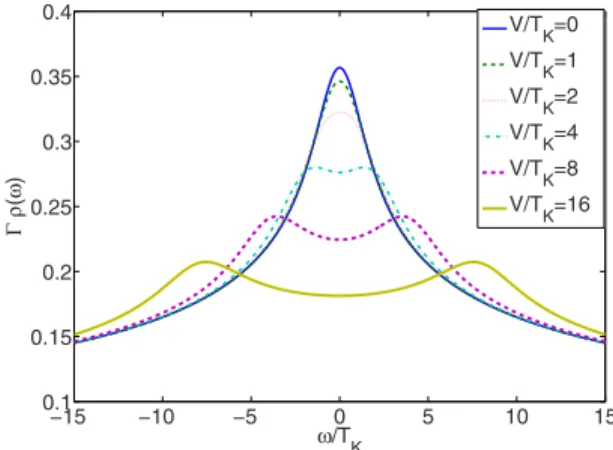
Out of equilibrium, the density of states in the dot is greatly influenced by the bias voltage or the difference be-tween the chemical potentials of the leads. Figure 3 reports our results for the nonequilibrium density of states, again in the particle-hole symmetric case at T/⌫=10−3 and U/⌫=4
for different values of the bias voltage V. In contrast with the
−150 −10 −5 0 5 10 15 0.1 0.2 0.3 0.4 0.5 0.6 0.7 ω/Γ Γρ (ω ) U=0 U=πΓ U=2πΓ U=3πΓ U=4πΓ U=5πΓ
FIG. 1. 共Color online兲 Equilibrium density of states in the particle-hole symmetric case at T/⌫=10−3 for different values of the parameter U 共the chemical potential of the lead eq is taken equal to 0兲. The density of states for large U shows a three-peak structure with two broad side peaks and a narrow Kondo resonance peak centered at the Fermi level.
−20 0 2 4 6 0.2 0.4 0.6 0.8 1 −εd/Γ G (2e 2/h) T/Γ=10−4 T/Γ=10−3 T/Γ=10−2 T/Γ=10−1
FIG. 2. 共Color online兲 Linear conductance as a function of dot-level energyd, for U/⌫=4 and at different temperatures. When the temperature is lowered, the conductance is enhanced in the singly occupied regime −d/⌫苸关0,4兴 and eventually reaches the maxi-mum conductance 2e2/h for a single channel at zero temperature. The conductance does not reach this limit here because of the nu-merical accuracy of the self-consistent treatment.
−15 −10 −5 0 5 10 15 0.1 0.15 0.2 0.25 0.3 0.35 0.4 ω/TK Γρ (ω ) V/T K=0 V/T K=1 V/T K=2 V/T K=4 V/T K=8 V/T K=16
FIG. 3. 共Color online兲 Nonequilibrium density of states in the particle-hole symmetric case at U/⌫=4 and T/⌫=10−3for different values of the bias voltage V. The chemical potentials of the two leads are taken equal toL/R=⫾V/2. The Kondo resonance peak splits into two side peaks located at= ⫾V/2, i.e., at the positions of the left- and right-lead chemical potentials. For convenience we choose to represent the two energy scales共energy and bias volt-age V兲 as normalized by the factor TK−1.
equilibrium situation, the Kondo resonance peak splits into two lower peaks pinned at the chemical potentials of the two leads. The reason is that the transitions between the ground state and the excited states of the dot are now mediated by the conduction electrons with energies lying close to the left-and right-lead chemical potentials.
We then compute the differential conductance as a func-tion of bias voltage for different temperatures and plot the results in Fig. 4. At low temperatures, the bias voltage de-pendence of the differential conductance shows a narrow peak at low bias 共zero-bias anomaly兲 reflecting the Kondo effect共mind the logarithmic horizontal axis兲, followed by a Coulomb peak centered around the value of the dot-level energy. Increasing temperature diminishes the intensity of the zero-bias peak, meaning that the Kondo effect is de-stroyed by temperature.
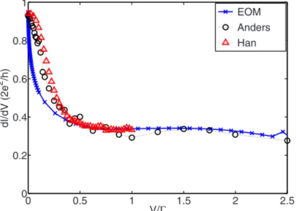
In order to discuss the universality of the dependence of the differential conductance on the bias voltage, we plot in Fig. 5 the results obtained at zero temperature for different values of the Coulomb interaction U. In the inset, the differ-ential conductance is found to be a universal function of the renormalized bias voltage V/TK, independent of other energy
scales such as U or⌫. This one-parameter scaling is obtained over a large range of V. Universality is lost around V ⬎10TK. Note that when V/TK⬍0.1, the unitary limit is not
completely recovered for the differential conductance due to the numerical accuracy in the self-consistency treatment, as was already mentioned before.
The physical origin of the destruction of the Kondo effect is the decoherence rates induced by the voltage-driven cur-rent. As we discussed in Sec. III B 2, these effects are well described by our EOM approach since it incorporates higher-order terms in t. They originate physically from the energy-conserving processes in which one electron hops onto the dot from the higher chemical potential while another electron hops out to the lower chemical potential. Since the processes involve two electrons hopping in and out, the lowest-order contribution is fourth order in t. These rates broaden and
diminish the Kondo resonance peaks in the density of states as the bias voltage increases, see Fig.3. Their effect leads to a decrease in the differential conductance when VⱖTK, as
was shown in Figs. 4 and 5. We will analyze this in more detail later in this section.
To further demonstrate that the method can work in a wide range of parameters, we report in Fig.6the differential conductance in the V −d plane in a three-dimensional plot.
The figure shows the usual Coulomb diamond defining in-side the Coulomb blockade regime N=1, where N is the total occupation number in the dot 共N=兺n兲. The bound-aries of the Coulomb diamond are related to the values of the renormalized dot-level energies⫾dand⫾d+ U共with some
additional renormalization effects in the mixed-valence re-gime兲. Within the Coulomb diamond along the V=0 line, one
10−2 10−1 100 101 102 0.1 0.2 0.3 0.4 0.5 0.6 0.7 0.8 0.9 V/TK dI/dV (2e 2/h) T/T K=0 T/T K=10 −1 T/T K=1 T/T K=10
FIG. 4. 共Color online兲 Differential conductance dI/dV versus the bias voltage V in the particle-hole symmetric case at U/⌫=4 for different values of temperature. The curves show a zero-bias peak, followed by the beginning of a broad Coulomb peak at large bias voltage. The differential conductance is reduced when either the temperature or the bias voltage increases, suggesting that the Kondo effect is suppressed by temperature or nonequilibrium effects.
FIG. 5. 共Color online兲 Differential conductance dI/dV versus the bias voltage V at T/TK= 0.1 in the particle-hole symmetric case for different values of U. The inset shows that the differential con-ductance as a function of normalized bias voltage V/TKscales to a single universal curve dI/dV= f共V/TK兲. At higher voltages, the uni-versal behavior is destroyed by a broad peak resulting from charge fluctuations. −2 0 2 4 −5 0 5 dI/dV (2e2/h) −εd/Γ V /Γ 0.1 0.2 0.3 0.4 0.5 0.6
FIG. 6. 共Color online兲 Color plot of the differential conductance dI/dV as a function of bias voltage V and dot-level energy dfor U/⌫=4 and T/⌫=10−3. The contour of the Coulomb peaks delimits the Coulomb blockade diamond, separating areas with well-defined dot occupation numberN ranging from 0, 1 to 2 at low V, and areas of charge fluctuations at high V. In theN=1 central valley, dI/dV shows a zero-bias peak typical of the Kondo effect.