Integrated emission inventory and modeling to assess distribution of particulate matter mass and black carbon composition in Southeast Asia

HAL Id: hal-01806837

https://hal.archives-ouvertes.fr/hal-01806837

Submitted on 16 Sep 2020

HAL is a multi-disciplinary open access

archive for the deposit and dissemination of

sci-entific research documents, whether they are

pub-lished or not. The documents may come from

teaching and research institutions in France or

abroad, or from public or private research centers.

L’archive ouverte pluridisciplinaire HAL, est

destinée au dépôt et à la diffusion de documents

scientifiques de niveau recherche, publiés ou non,

émanant des établissements d’enseignement et de

recherche français ou étrangers, des laboratoires

publics ou privés.

Integrated emission inventory and modeling to assess

distribution of particulate matter mass and black carbon

composition in Southeast Asia

Didin Agustian Permadi, Nguyen Thi Kim Oanh, Robert Vautard

To cite this version:

Didin Agustian Permadi, Nguyen Thi Kim Oanh, Robert Vautard. Integrated emission inventory and

modeling to assess distribution of particulate matter mass and black carbon composition in Southeast

Asia. Atmospheric Chemistry and Physics, European Geosciences Union, 2018, 18 (4), pp.2725 - 2747.

�10.5194/acp-18-2725-2018�. �hal-01806837�

https://doi.org/10.5194/acp-18-2725-2018 © Author(s) 2018. This work is distributed under the Creative Commons Attribution 3.0 License.

Integrated emission inventory and modeling to assess

distribution of particulate matter mass and black carbon

composition in Southeast Asia

Didin Agustian Permadi1, Nguyen Thi Kim Oanh1, and Robert Vautard2

1_{Environmental Engineering and Management, School of Environment, Resources and Development,}

Asian Institute of Technology, Klong Luang, Pathumthani 12120, Thailand

2_{Laboratoire des Sciences du Climate de l’Environment (LSCE), Institut Pierre Simon Laplace (IPSL), Gif-sur-Yvette, France}

Correspondence: Nguyen Thi Kim Oanh (kimoanh@ait.ac.th) Received: 5 April 2017 – Discussion started: 2 May 2017

Revised: 25 November 2017 – Accepted: 3 December 2017 – Published: 26 February 2018

Abstract. This is part of a research study addressing the potential co-benefits associated with selected black carbon (BC) emission reduction measures on mitigation of air pol-lution and climate forcing in Southeast Asia (SEA). This pa-per presents details of emission inventory (EI) results and WRF–CHIMERE model performance evaluation. The SEA regional emissions for 2007 were updated with our EI re-sults for Indonesia, Thailand, and Cambodia and used for the model input. WRF–CHIMERE-simulated 2007 PM10,

PM2.5, and BC over the SEA domain (0.25◦×0.25◦) and

the results were evaluated against the available meteorology and air quality monitoring data in the domain. WRF hourly simulation results were evaluated using the observed data at eight international airport stations in five SEA countries and showed a satisfactory performance. WRF–CHIMERE results for PM10 and PM2.5 showed strong seasonal

influ-ence of biomass open burning while the BC distribution showed the influence of urban activities in big SEA cities. Daily average PM10constructed from the hourly

concentra-tions were obtained from the automatic monitoring staconcentra-tions in three large SEA cities, i.e., Bangkok, Kuala Lumpur, and Surabaya, for model evaluation. The daily observed PM2.5

and BC concentrations obtained from the Improving Air Quality in Asian Developing Countries (AIRPET) project for four cities (i.e., Bangkok, Hanoi, Bandung, and Manila) were also used for model evaluation. In addition, hourly BC con-centrations were taken from the measurement results of the Asian Pacific Network (APN) project at a suburban site in Bangkok. The modeled PM10 and BC satisfactorily met all

suggested statistical criteria for PM evaluation. The modeled

PM2.5/PM10 ratios estimated for four AIRPET sites ranged

between 0.47 and 0.59, lower than observed values of 0.6– 0.83. Better agreement was found for BC/PM2.5ratios with

the modeled values of 0.05–0.33 as compared to the obser-vation values of 0.05–0.28. AODEM (extended aerosol op-tical depth module) was used to calculate the total colum-nar aerosol optical depth (AOD) and BC AOD up to the top of the domain at 500 hPa (∼ 5500 m), which did not include the free-tropospheric long-range transport of the pollution. The model AOD results calculated using the internal mix-ing assumption were evaluated against the observed AOD by both AERONET and MODIS satellite in 10 countries in the domain. Our model results showed that the BC AOD contributed 7.5–12 % of the total AOD, which was in the same range reported by other studies for places with inten-sive emissions. The results of this paper are used to calculate the regional aerosol direct radiative forcing under different emission reduction scenarios to explore potential co-benefits for air quality improvement, reduction in the number of pre-mature deaths, and climate forcing mitigation in SEA in 2030 (Permadi et al., 2017a).

1 Introduction

Southeast Asia (SEA), with a large population and fast-growing economy, is an important contributor to the emis-sions of air pollution and greenhouse gases in Asia (Streets et al., 2003; Zhang et al., 2009). The emissions of

anthro-2726 D. A. Permadi et al.: Modeling PM and BC distributions in Southeast Asia pogenic aerosol from Asia, and specifically from SEA, are

expected to rise in the near future due to the increase in the energy demand and rapid industrialization (Lawrence and Lelieveld, 2010; Ohara et al., 2007). High levels of fine par-ticulate matter (PM with diameter less than 2.5 µm or PM2.5),

the most detrimental air pollutant affecting health (Janssen et al., 2011; WHO, 2012), are observed in many develop-ing Asian cities, with the annual average often exceeddevelop-ing the WHO guideline of 10 µg m−3by many times (Kim Oanh et al., 2006; Hopke et al., 2008). Components of PM, e.g., PM2.5, PM10(PM with diameter less than 10 µm), black

car-bon (BC), and organic carcar-bon (OC), have been monitored in some Asian cities and the results, although fragmented, showed considerably high levels (Kondo et al., 2009; Kim Oanh et al., 2006; Hopke et al., 2008). The fine particles and their precursors are also involved in long-range trans-port (LRT), hence causing regional phenomena such as at-mospheric brown clouds (ABC) (UNEP and C4, 2002; Ra-manathan et. al., 2001) and affecting the climate (UNEP-WMO, 2011). Globally, measures aiming to reduce emis-sions of BC (and co-emitting pollutants) were shown to re-duce the number of premature deaths and slow down the near-future temperature increase, in addition to other bene-fits to be gained in Asia, where current emissions are high (UNEP-WMO, 2011; Shindell et al., 2012).

To comprehensively assess the co-benefits of emission re-duction measures on a regional scale, finer temporal and spa-tial resolutions of the modeling results are required. Several studies have been conducted for various Asian domains using a regional climate model with chemistry (Nair et al., 2012) or chemical transport models (CTMs) with an additional aerosol optical module. Most of the Asian regional modeling studies mainly focused on the domains of East (Han et al., 2011; Park et al., 2011; Chen et al., 2013; Zhang et al., 2016), South (Goto et al., 2011), and continental East and Southeast Asia (Lin et al., 2014). These studies also highlighted several challenges for models to reproduce the ground-observed PM due to inaccurate emission inventory (EI), simulated meteo-rological fields, and the extent of model representations (e.g., secondary organic aerosol formation, gas–particle partition-ing, dry and wet deposition).

There are currently no detailed modeling studies con-ducted for the SEA domain, especially maritime SEA, which includes Indonesia with its large biomass open burning (OB) emissions. For such a modeling effort, first a reasonably ac-curate regional EI database should be prepared to generate input data. Several global and regional EI databases are avail-able which also cover the SEA domain. These datasets have been developed using the activity data taken from several in-ternational data sources (Zhang et al., 2009; EC-JRC/PBL, 2010) or based on the results of large-scale energy models (Streets et al., 2003). Efforts therefore should be put forward to update the SEA EI databases in order to generate emission input data for SEA regional modeling studies.

Our research used integrated EI and modeling tools to provide the spatial and seasonal distributions of aerosol species (PM10, PM2.5, and BC) in SEA for 2007 and the

co-benefits (for air quality, health, and climate forcing) of selected emission reduction measures for 2030. This paper presents the SEA emissions for the base year of 2007 and the WRF–CHIMERE performance evaluation. CHIMERE (Menut et al., 2013, and references therein) was used to simulate three-dimensional (3-D) aerosol concentrations in the domain using the meteorological fields generated by the Weather Research and Forecasting (WRF) model (Micha-lakes et al., 2004). The model results were evaluated us-ing available ground-based measurements of PM10, PM2.5,

and BC in several SEA cities. The extended aerosol opti-cal depth (AOD) module (AODEM), detailed in Landi and Curci (2011), was applied to calculate the total columnar AOD and BC AOD. The modeled total AOD was evaluated using the observed AOD from both ground-based Aerosol Robotic Network (AERONET) and the Moderate Resolution Imaging Spectroradiometer (MODIS) satellite product. The results are used in the follow-up study, which investigated the potential co-benefits of various emission reduction mea-sures implemented in Indonesia and Thailand for air qual-ity improvement, reduction of premature deaths, and climate forcing mitigation in 2030 (Permadi et al., 2017a).

2 Methodology

2.1 Emission inventory and emission input data The emissions from major anthropogenic sources in Indone-sia, Thailand, and Cambodia were developed following the EI framework given in the Atmospheric Brown Cloud Emis-sion Inventory Manual (ABC EIM) (Shrestha et al., 2013) using the activity data summarized in Table 1. A detailed EI methodology for Indonesia was presented in Permadi et al. (2017b).

The biomass OB categories considered in this study in-cluded crop residue open burning (CROB) and forest fires (aboveground forest fires and peatland fires). The CROB emissions (aerosol and trace gases) for Thailand for 2007 were taken from Kanabkaew and Kim Oanh (2011), and both CROB and aboveground forest fire emissions for In-donesia were from Permadi and Kim Oanh (2013), also for 2007. For Cambodia, CROB emissions for 2007 were also in-cluded in the inventory (Permadi, 2013) but forest fire emis-sions were taken from the Global Fire Emission Database v3 (GFEDv3) database (van der Werf et al., 2010). CROB emissions for Thailand, Indonesia, and Cambodia were es-timated from crop production statistics, residue to crop ra-tio, dry matter to crop residue rara-tio, fraction of biomass burned in the field, combustion efficiency, and emission fac-tors. The emission results were higher than other databases that used the MODIS product (e.g., GFEDv3) because the

Table 1. Summary of activity data level from different emission sources in three countries.

Sectors Types of activity data Activity data

Indonesia Thailand Cambodia Power generation Fuel consumption (Mt yr−1)

Coal 23.4 20.5 –

Natural gas 3.2 29.8 –

Fuel oil 9.4 0.75 0.62

Biomass 6.3 – –

Manufacturing industry Fuel consumption (Mt yr−1)

Coal 5.4 12.3 –

Gasoline 0.34 0.013 –

Fuel oil 1.8 2.4 0.52

Biomass – 20.7 –

On-road transport Number of registered vehicles 48 26 1.9 (million yr−1)

Air traffic LTO (× 1000 yr−1) 344 555 39 Residential and commercial Fuel consumption (Mt yr−1)

Coal 0.028 – – Wood 100.5 7.6 0.4 Kerosene 7.3 0.13 0.003 LPG 1 1.15 0.005 Charcoal 20.4 3.9 0.042 Other biomass – 0.14 –

Fugitive emissions from fuel Coke production (Kt yr−1) 182 – – Gas production (Tg yr−1) 8654 31.24 – Oil production (Tg yr−1) 29 6.2 – Gasoline distributed (Mt yr−1) 13.7 5.4 – Agro-residue open burning Total dry crop residue openly burned (Mt yr−1) 43.5 18.2 4.3 Forest fire Total forest area burned, including peatland fire

(ha yr−1)

545 881 1 851 850 98 761

Solid waste open burning Total dry solid waste burned (Mt yr−1) 1.26 0.28 0.175 Agriculture-related activities Total number of livestock population (head, ×106) 1359 328 22.3 Fertilizer consumption (Mt yr−1) 6.8 3.6 – Solvent and product use Paint (Kt yr−1of paint) 606 ne ne

Degrease (t yr−1of solvent consumed) 103 Chemicals (Kt yr−1of products) 1269 Other products use (i.e., ink, domestic solvent,

glue and adhesives) (Kt of products)

161

satellite may not efficiently capture short-lived, small-sized, sporadic CROB fires (Permadi and Kim Oanh, 2013). For other countries in the domain, the emissions from the above-ground forest fires were from Song et al. (2009) while those from CROB were from GFEDv3 for the base year of 2007. The 2007 emissions from peatland fires of all countries in the SEA domain were also taken from GFEDv3 (van der Werf et al., 2010). The GFEDv3 database was developed using a combination of MODIS burned area and active fire

prod-ucts, which is believed to better detect the peatland fires than the MODIS burned area product MCD45A1 alone for forest fire detection (Shi et al., 2014).

Biogenic emissions were calculated online by the CHIMERE model using the methodology described in Simp-son et al. (1999) that considers seaSimp-sons and vegetation cover types taken from the Global Land Cover Facility (GLCF) (http://glcf.umd.edu) with a resolution of 1 km × 1 km. CHIMERE incorporates the Model of Emissions of

2728 D. A. Permadi et al.: Modeling PM and BC distributions in Southeast Asia Gases and Aerosol from Nature (MEGAN) module

(Guen-ther et al., 1995) for estimation of volatile organic com-pounds (VOCs) from natural vegetation and NO emissions from soil. We did not include the emissions from interna-tional shipping in this simulation, but “inland waterway” sources were included in the inventories for the three coun-tries. Other sources of PM such as unpaved road and wind-blown dust emissions were also not included in this study.

Spatial distributions were made based on source activ-ity data or relevant proxies collected for the administrative boundaries. For example, for Indonesia, the emissions were disaggregated at the district level (300 districts), while for Thailand and Cambodia emissions were presented for the provincial level (76 and 24 provinces, respectively). Further, the emissions were gridded into 0.25◦×0.25◦using the Ge-ographic Information System (GIS) tool. For other countries in SEA, the emissions of SO2, NOx, CO, VOC, PM10, PM2.5,

BC, and OC were taken from the available online gridded EI databases (grid size of 0.5◦, i.e., ∼ 50 km) compiled by the Center for Global and Regional Environmental Research (CGRER) (Zhang et al., 2009). The gridded CH4and NH3

emissions that were not included in CGRER were taken from the global Emission Database for Global Atmospheric Re-search (EDGAR) (EC-JRC/PBL, 2010), with a grid resolu-tion of 10 km×10 km. Emissions from all considered sources were compiled for the base year of 2007 and were gridded to 0.25◦×0.25◦(∼ 30 km × 30 km) for the modeling input.

Monthly based activity data were obtained whenever avail-able to construct monthly emissions, but when the data were not available relevant proxies were used. Specific coun-try hourly variations of emissions were extracted from the available studies in SEA. For Indonesia, detailed method-ology and data sources to construct monthly and hourly emissions of major anthropogenic sources are detailed in Permadi et al. (2017b). For aboveground forest vegetation, crop residue, and municipal solid waste OB emissions, the monthly and hourly profiles were adopted from Permadi and Kim Oanh (2013). For Thailand, the hourly profiles for power plants and industry were obtained from Pham et al. (2008) while those for other major anthropogenic sources were taken from Vongmahadlek et al. (2009). The survey-based information on hourly profiles reported in Kan-abkaew and Kim Oanh (2011) was used for CROB emis-sions. For other countries, relevant data from regional EI from Streets et al. (2003) were utilized. The hourly emission input for the domain were prepared using a Fortran program developed at the Asian Institute of Technology (AIT) for this purpose.

The lumping of non-methane volatile organic com-pounds (NMVOCs) emissions into the model species was done according to the MELCHIOR mechanism (Middle-ton et al., 1990). The aggregation produced the emissions of 33 species, including trace gases and aerosol in units of mol cm−2s−1. Aerosol fluxes were also converted to the “molecule-like” units in the emission input data using a

fic-tive molar mass equal to 100 g mol−1 (Bessagnet et al., 2004).

2.2 Modeling domain

The choice of domain size and resolution affects the balance between the boundary and internal modeling forcing in the simulated concentrations (Seth and Giorgi, 1998). For this study, it is important that the defined domain allows the trans-port of air pollutants by the monsoon circulation across SEA. Therefore, we set the domain to cover as much as possible the major upwind emission sources and to capture meteorologi-cal processes in the region of interest.

The SEA domain horizontally covered nine countries of the Association of Southeast Asian Nations (ASEAN) and three provinces of Southern China (Fig. S1 in the Supple-ment). The WRF domain extended from central Myanmar to northern Australia, covering 230×200 grids. The CHIMERE domain extended from Southern China (24◦N, 95◦E) to east-ern parts of Indonesia (9◦S, 137◦E), consisting of 169 × 133 grids. The grid resolution of the WRF and CHIMERE was set to be the same, 0.25◦×0.25◦(∼30 km ×30 km). 2.3 WRF and CHIMERE model configuration

WRF version 3.3 was used with lateral boundaries and ini-tial meteorological conditions taken from the National Cen-ters for Environmental Prediction (NCEP) final (FNL) global analyses that are available at 1◦×1◦ grid resolution every 6 h (http://rda.ucar.edu/datasets/ds083.2/). The WRF Prepro-cessing System (WPS) of geographical input data (i.e., land use, vegetation index, soil type, and albedo) was also ob-tained from the NCEP database. In total, 28 vertical lev-els were simulated, with the lowest level having the physi-cal height of about 38 m. Analysis nudging was performed in the planetary boundary layer (PBL) and other layers for wind components (u and v), temperature (T ), and relative humidity (RH). Nudging coefficients were set for all param-eters at 0.00005 s−1. The time interval between analyses was set at 360 min, which is equivalent to the 6-hourly bound-ary input data used in our study. This analysis nudging was performed because it is suitable for coarse-resolution simu-lations (30 km × 30 km) to drive regional air quality models since it can improve the accuracy for the downscaled and/or nested fields (Dudhia, 2012; Bowden et al., 2012). Note that, due to the insufficiency of spatially distributed meteorologi-cal observations in the domain, the observation nudging was not performed.

In the WRF simulation, the following physics options were used: simple ice microphysics, unified Noah Land Surface Model for the land-surface scheme, Rapid Radiative Trans-fer Model (RRTM) and Dudhia schemes for long- and short-wave radiation, a PBL parameterization scheme from Yonsei University, and a Kain–Fritsch scheme with deep and shal-low convection option for cumulus parameterization. These

schemes were selected as they are suitable for mesoscale grid size and have been used in previous studies (Jankov et al., 2005; Osuri et al., 2012).

This study used CHIMERE version 2008c with the MEL-CHIOR 2 chemical mechanism that was adapted from the original European Monitoring and Evaluation Programme (EMEP) and consisted of around 120 reactions and 40 chem-ical species. The vertchem-ical profiles of updated reaction rates in MELCHIOR 2 have been developed using tabulated clear-sky photolysis rates taken from the Tropospheric Ultraviolet and Visible (TUV) model (EC4MACS, 2012). This version of CHIMERE has an aerosol module which consists of the total primary PM emissions (BC, OC, and other primary par-ticles) and secondary inorganic PM species, such as nitrate, sulfate, ammonium, and secondary organic aerosol (Bessag-net et al., 2004). CHIMERE applies the sectional approach to discretize particle size distribution into a finite number of bins. The considered particle size range was from 40 nm to 10 µm, which were distributed into eight bins (0.039, 0.078, 0.156, 0.312, 0.625, 1.25, 2.5, 5, 10 µm) (Pere et al., 2011). Most of aerosol-related dynamic processes, such as conden-sation, coagulation, wet and dry deposition, adsorption, and scavenging, are incorporated in the model (http://www.lmd. polytechnique.fr/chimere/). This version of CHIMERE only allows tropospheric simulations below 200 hPa (∼ 12 km).

We used eight vertical layers in this study, from sigma level 0.999 (∼ 20 m) to ∼ 0.5 (∼ 5500 m), equivalent to the 500 hPa pressure level. This upper limit was selected based on a suggestion that in the modeling of anthropogenic pollu-tion, extending the vertical dimension beyond 500 hPa would not substantially change the modeled aerosol concentrations for the ground level (Menut et al., 2013). However, it is rec-ognized that the top of the domain at 500 hPa may not be able to include the free-tropospheric LRT of the pollution and it brings in uncertainty to the total column AOD results. Note that in the CHIMERE version used in this study, the photolysis rates are calculated under clear-sky conditions as a function of height using the TUV model (Madronich et al., 1998) and photolysis rates are estimated only up to 9000 m. However, with the present formulation for cloud–radiation photolysis, assuming that the model domain is below the cloud, cloud albedo was not taken into account. Monthly mean boundary conditions of gases and aerosol were taken from the simulation results for a period of 1998–2002 by the Laboratoire de Météorologie Dynamique (LMDZ) – In-teraction avec la Chimie et les Aérosols (INCA) (Schulz et al., 2006), which are available at the CHIMERE website. To assess the effects of the somewhat aged boundary condi-tions compared to the model year, a comparison between the monthly average concentrations at the boundaries between 2007 and 1998–2002 was made which showed that the dif-ference among the datasets differed by 0.98–1.23 consider-ing the ratios for aerosol and PM precursor gases (i.e., BC, OC, NO2, CO, SO2, C2H4, CH3CHO, and NH3) between

the two datasets. This implies that basically the two datasets

were almost similar. Thus, the impacts of the aged boundary conditions on the simulation are expected but with a small magnitude. Initial conditions of gases and aerosol concentra-tions in every grid were interpolated from the outputs of the global CTM of the LMDZ-INCA simulation. A 1-year simu-lation (1 January–31 December 2007) was performed by both WRF and CHIMERE with a spinup period of 1 week prior to the main simulation period.

2.4 Aerosol optical depth calculation

A standalone post-processing tool, known as AODEM, de-veloped by Istituto di Scienze dell’Atmosfera e del Clima – Consiglio Nazionale delle Ricerche (ISAC-CNR) of Italy (Landi and Curci, 2011) was used to calculate optical pa-rameters of AOD (extinction coefficients and single scatter-ing albedo) usscatter-ing the 3-D aerosol species mass concentra-tion fields output of WRF–CHIMERE for different size bins. AODEM calculates 3-D particle number concentrations from these mass concentrations and provides the extinction coef-ficients for each grid cell, assuming the spherical shape of particles (Landi, 2013). Three options of the aerosol mixing state were provided in AODEM: external, internal homoge-neous, and internal coated spheres. Aerosol optical properties are simulated by AODEM following the Mie theory (Bohren and Huffman, 1983) for the wavelength range from 340 to 1640 nm. We selected the “aerosol internal mixing” option in the calculation because existing field measurements con-firmed that aerosol is typically found in the internally mixed state (Lesins et al., 2002) largely due to coagulation and growth of aerosol particles (Jacobson, 2000). Note that AOD was calculated from the surface to the model’s top layer of 500 hPa; hence it could not represent the transport through the convective processes taking place above the model top layer or the LRT in the free troposphere mentioned above.

For calculation of optical aerosol properties, AODEM pro-vides the particle number concentrations separately for five components: BC, OC, sea salt, dust, and secondary inorgan-ics (nitrate, sulfate, and ammonium). The AOD scattering was simulated using “brute force” by excluding BC in the simulation (Landi and Curci, 2011). BC AOD was calculated by subtracting the AOD scattering from the total AOD. 2.5 Model evaluation

The evaluation of WRF outputs was done using observed data from eight airport meteorological stations in five SEA countries that captured major subclimate zones (upper, near-Equator, and lower latitude) in the domain. Hourly obser-vations from all these airport stations in 2007 were ob-tained from http://weather.uwyo.edu/surface/meteorogram/. The statistical evaluation of WRF outputs was done us-ing the criteria provided by Emery et al. (2001), which in-clude the mean bias error (MBE), mean absolute gross error (MAGE), and root mean square error (RMSE). The

mod-2730 D. A. Permadi et al.: Modeling PM and BC distributions in Southeast Asia eled surface pressure and upper wind fields (at 850 hPa)

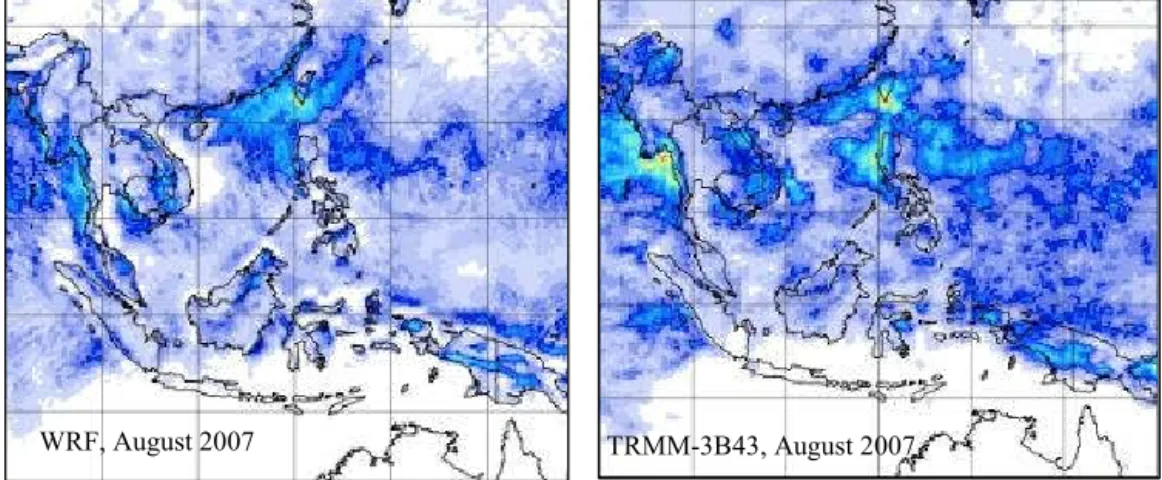
were compared with the European Centre for Medium-Range Weather Forecasts (ECMWF) Reanalysis (ERA) Interim data extracted from http://apps.ecmwf.int/datasets/ for the same vertical levels. Simulated monthly accumulated precipita-tion fields were compared with the satellite-based obser-vations provided by the Tropical Rainfall Measuring Mis-sion (TRMM-3B43) (https://disc.sci.gsfc.nasa.gov/datasets/ TRMM_3B43_V7/summary?keywords=TRMM).

Only limited air pollution data were available in SEA for the model performance evaluation. This study collected the observed concentrations of aerosol (BC, OC, PM2.5, and

PM10) and related gases from various sources. For

exam-ple, daily (24 h) concentrations of PM10, PM2.5, BC, and

OC in four SEA cities (i.e., Manila, Hanoi, Bandung, and Bangkok) in 2007 were taken from the measurement data generated by the Improving Air Quality in Asian Develop-ing Countries (AIRPET) project “ImprovDevelop-ing Air Quality in Asian Developing Countries” (Kim Oanh et al., 2006, 2014). Hourly BC and OC concentrations were taken from the mea-surement results of the Asian Pacific Network (APN) project at the AIT located in Pathumthani province of the Bangkok Metropolitan Region, Thailand (Kondo et al., 2009). Hourly PM10in Bangkok (Thailand), Kuala Lumpur (Malaysia), and

Surabaya (Indonesia) in 2007 were collected from the respec-tive national monitoring networks. The statistical evaluation of simulated aerosol levels was done using mean fractional bias (MFB) and mean fractional error (MFE) (Boylan and Russel, 2006). Definitions of the statistical measures used in the model performance evaluation are given in Table S1 in the Supplement.

The monthly AERONET data for 2007 were downloaded from the National Aeronautics and Space Administration (NASA) website (http://aeronet.gsfc.nasa.gov/) for the evalu-ation of the modeled AOD. The AERONET data were level 2 quality controlled and recorded at 10 AERONET stations (using a sun photometer) listed in Table S2 in the Supple-ment. This AERONET dataset has already been pre- and post-field calibrated with cloud screening and quality assur-ance. The selected 10 AERONET stations had more com-plete datasets in 2007 and they represent all subclimate zones in the domain. The sun photometer measures AERONET AOD at six different wavelengths (1020, 870, 675, 500, 440, and 380 nm). Therefore, to compare with the modeled AOD at 550 nm, the AERONET AOD at 500 nm was converted to that 550 nm using a logarithmic interpolation (Chung et al., 2012).

For a qualitative evaluation of the spatial distributions we checked the consistency between the modeled AOD spatial distribution over the SEA domain and the monthly MODIS AOD (level 3 data measured at 550 nm wave-length downloaded from https://giovanni.sci.gsfc.nasa. gov/giovanni/#service=TmAvMp&starttime=&endtime= &variableFacets=dataFieldMeasurement%3AAerosol% 20Optical%20Depth%3B).

3 Results and discussion 3.1 Base year emissions

The obtained total national emission estimates of Indone-sia, Thailand, and Cambodia for 2007 were compared with the existing regional EI databases of EDGAR for 2007 and CGRER for 2006. Table 2 shows a reasonable agreement in the ranges of the estimates between the emission databases for three countries: Cambodia, Indonesia, and Thailand. De-tailed EI results for Indonesia were presented in Permadi et al. (2017b). There are certain discrepancies between the databases that may be explained by several factors, includ-ing the uncertainty in activity data levels and emission fac-tors used as well as the different coverage of the emission sources by different EI works. Specifically, for the emission sources of N2O, our EI for the three countries did not cover

the direct emissions from cultivated soil (fertilized land) and the indirect N2O emissions from agriculture-related

activi-ties (microbial nitrification and denitrification), hence result-ing in lower N2O emission estimates. Similar reasoning may

be used to explain our lower estimates for CH4as compared

to EDGAR for all three countries.

For Indonesia, our emission estimates were between those of CGRER and EDGAR for a number of species. The es-timates for PM10, PM2.5, and BC actually agreed well

be-tween these databases while OC of CGRER appeared to be higher. However, the SO2 estimates differed a lot between

the databases and our value was lower than others (mainly for on-road transportation and industry), which may be at-tributed to a more bottom-up approach used in our EI that relied on actual sulfur content used in the country and im-plementation of air pollution control devices (Permadi et al., 2017b). For example, our SO2estimate for the power plants

of Indonesia was 300 Gg yr−1, which was more comparable with the CGRER estimate (409 Gg yr−1) but much lower than the EDGAR estimate (1000 Gg yr−1). The most striking dif-ference was for the CO2 emissions, which showed a much

higher value by EDGAR; this could be clearly explained by the inclusion of two major sources in the EDGAR dataset: (i) the forest fire post-burn decay (698 000 Gg yr−1) and (ii) de-cay of drained peatland (504 000 Gg yr−1). If these two emis-sion sources are excluded from the EDGAR results, the CO2

estimates of all three databases are similar for Indonesia. The EI results for Thailand and Cambodia also showed reason-able agreements between the availreason-able datasets, except for CO2, which was estimated higher by EDGAR for

Cambo-dia. The BC and OC emissions for these two countries were mostly comparable, i.e., differing by a factor less than 2.0 among the datasets.

Table 2. EI results for base year in comparison with the existing regional EI datasets (Gg yr−1).

Species Indonesia Thailand Cambodia Other SEA Southern Total This studya EDGARb CGRERc This studya EDGARb CGRERc This studya EDGARb CGRERc countriesd part of China domain SO2 997 2433 1499 827 721 961 41 42 34 2695 6204 10 781 NOx 3282 2162 1896 701 882 1086 97 92 27 2623 4166 10 910 CO 24 169 32 246 26 703 9095 12 553 10 815 2877 2453 570 19 054 33 377 89 252 NMVOC 3840 4528 8225 1120 525 3052 331 18 113 5644 4441 15 613 NH₃ 1258 1617 1390 469 675 388 110 95 86 1543 2247 5645 CH4 3950 10 300 6443 1053 4541 3567 713 1969 708 13 833 14 640 34 218 PM10 2046 3454 1838 782 1196 474.9 115 268 68 1763 3644 8458 PM2.5 1644 2023 1609 607 781 388.5 65 201 61 1466 2653 6519 BC 226 173 229 47 73 72 7 13 7 159 362 821 OC 674 711 1246 240 234 364 40 73 32 604 643 2245 CO₂ 508 022 1 700 450 587 000 260 988 235 644 351 000 28 296 185 211 36 000 856 225 1 406 860 3 092 654 (514 882) (229 500) (174 300) N2O 180 329 ne 84 71 ne 60 73 ne 271 346 941

Note: ne means not estimated

a_{EI conducted for base year of 2007 using the ABC EIM framework (Shrestha et al., 2013). Detailed methodology and results were presented in Permadi et al. (2017a).} b_{EDGAR for base year of 2007 (Olivier et al., 2001). Retrieved from http://edgar.jrc.ec.europa.eu/overview.php?v=42FT2012. The CO}

2emissions, excluding forest fire post

burn decay and decay of drained peatland, are given in brackets for comparison with our estimates.

c_{CGRER for base year of 2006 (Zhang et al., 2009). Retrieved from https://cgrer.uiowa.edu/projects/emmison-data. For NH}

3, CH4, and CO2,

emissions were taken from CGRER inventory in 2000 (Streets et al., 2003). Peatland fire for SEA for 2007 was taken from GFED v3.

Retrieved from https://daac.ornl.gov/cgi-bin/dsviewer.pl?ds_id=1191.dOther SEA countries include Brunei, Lao PDR, Malaysia, Myanmar, Philippines, Singapore, and Vietnam.

The emission shares by source category for the three coun-tries are presented in Fig. S2 in the Supplement. The emis-sions of aerosol species (PM10, PM2.5, BC, and OC) were

mainly from the residential and commercial combustion in Indonesia (43–80 %) and Cambodia (55–78 %) while for Thailand the biomass OB (forest fire and crop residue) emis-sions were dominant, i.e., 31–74 %. For SO2, the emission

in Indonesia were mainly contributed by the transport sec-tor (36 %) and thermal power plants (33 %) but the indus-try was the main contributor in both Thailand (66 %) and Cambodia (33 %). For NOx, the total emissions in

Indone-sia were dominated by the fugitive emissions from oil and gas operation (44 %), in Thailand by power plants (34 %), and in Cambodia by forest fires (60 %). The total emission of NH3, an important precursor for PM2.5, in all three countries

were mainly from manure management and fertilizer appli-cation, i.e., 63 % for Indonesia, 75 % for Thailand, and 78 % for Cambodia.

The emissions from other SEA countries and from the non-SEA part of the domain (southern part of China) used in our modeling study are also included in Table 2. The sions from Southern China had high shares in the total emis-sions from the modeling domain. It is seen that Indonesia and Thailand were collectively the largest emitters of all pol-lutants, sharing of 25–66 % of 2007 SEA emissions and 17– 44 % of the modeling domain emissions. Thus, emission re-duction measures implemented for these two countries are expected to contribute remarkably to air quality improvement in the region, which will be analyzed in the companion pa-per (Permadi et al., 2017a). The spatial distributions of the annual average emissions of BC and CO at 0.25◦×0.25◦ (∼ 30 km × 30 km) resolution are presented in Fig. 1, show-ing higher emission intensity over large urban areas in the domain.

3.2 WRF model results and evaluation

3.2.1 Model statistical performance evaluation

The WRF hourly outputs, including surface T , RH, and wind speed (WS) for 2007, were compared with the observed data at eight international meteorological stations in five SEA countries (Table 3). The comparison was done for two sea-sons: 3 months, 1 January–31 March, to represent the dry season in the continental SEA (but the wet season in Indone-sia) and 3 months, 1 August–31 October, to represent the wet season in the continental SEA (but the dry season in Indone-sia). The time series of daily average modeled vs. observed meteorological parameters, as shown in Fig. S3a and b in the Supplement, showed that the model appeared to reasonably reproduce all parameters for the considered stations. In gen-eral, the model performance for T and WS simulations at all the stations was better than for RH during both periods.

The statistical performance evaluation for the hourly sim-ulated values against the MBE, MAGE, and RMSE crite-ria is given in Table 3. MBE for the January–March period range was −1.9–+0.7◦C for T , −0.3–+2.7 m s−1 for WS, and −7.1–+7.7 % for RH. The corresponding range obtained for the August–October period was −0.1–+2.3◦C, −0.6– +2.1 m s−1, and −5.4–+2.6 %. Other statistical measures of MAGE and RMSE varied between the stations and the devi-ations from the suggested criteria were generally small. This suggested a relatively good model performance of WRF for both dry and rainy seasons. Overall, for the stations located in the northern latitudes (above the Equator line), the model performed better in the wet season (August–October), while for those located near and lower than the Equator line the model performance was equally good for both dry and wet seasons. The discrepancy between model results and

obser-2732 D. A. Permadi et al.: Modeling PM and BC distributions in Southeast Asia

Table 3. Statistical parameters for WRF model performance evaluation for two periods (bold values are those meeting the evaluation criteria). Station Statistical parameters

MBE MAGE RMSE N

RH T WS RH T WS RH T WS

(%) (◦C) (m s−1) (%) (◦C) (m s−1) (%) (◦C) (m s−1) Jan–Mar 2007

Olongapo, Philippines 5.4 −0.9 1.3 15.8 3.1 0.18 19.3 3.9 2.7 1861 Davao, Philippines −4 −1.6 2.7 10.4 2.8 2.9 12.6 3.6 3.4 1250 Don Muang, Thailand −13 −0.4 1 16 2.5 1.6 18.5 3.8 2 2148 Trat, Thailand 5.7 −1.9 1.6 12.7 3.1 3.1 15.2 3.7 3.6 996 Pnom Penh, Cambodia 7.7 0.7 0.5 15.5 3.6 2.1 18.1 4.5 2.6 1513 Jakarta, Indonesia −7.1 −0.8 0.7 14.5 3.2 2.1 19.7 4.2 2.6 2036 Kuala Lumpur, Malaysia −2.5 −0.14 0.14 6.8 1.2 1.1 10.3 2.2 1.4 2143 Sarawak, Malaysia −1.8 −0.13 −0.3 5.6 1.2 0.9 9.2 2.1 1.2 2148 Aug–Oct 2007

Olongapo, Philippines 1.5 2.3 0.5 8.3 2.5 1.3 17.6 3.5 3.1 1958 Davao, Philippines −0.81 −0.13 0.2 6.4 2.2 0.7 12.8 4.8 1.3 1262 Don Muang, Thailand 2.6 −0.4 −0.1 11.1 2.1 1.4 15.4 3.5 2.2 2139 Trat, Thailand 0.86 −0.1 2.1 5.4 1.3 2.7 11.6 3.8 3.3 1017 Pnom Penh, Cambodia −6.7 0.7 0.1 10.1 1.7 1.1 14.6 3.4 1.7 1602 Jakarta, Indonesia 0.8 2.3 0.47 5.6 2.4 2.3 11.2 3.3 3.1 1958 Kuala Lumpur, Malaysia −5 0.3 −0.1 10.4 1.5 0.98 13.2 1.9 1.23 2159 Sarawak, Malaysia −5.4 −0.1 −0.6 8.9 3.5 1.1 11.56 4.2 1.4 2159 Note: bolded values represent satisfactorily model output. Criteria for MBE: WS ≤ ±0.5 m s−1, T ≤ ±0.5◦C, RH ≤ ±10 %. Criteria for MAGE: T ≤ 2◦C, RH ≤ 2 %. Criteria for RMSE: WS ≤ 2 m s−1. N is the number of data points. Description of the statistics measures is presented in Table S1 in the Supplement.

vations was perhaps partly due to the fact that the domain covers some regions, such as the Indonesian maritime conti-nent, that are principally characterized by active convection with a frequent presence of deep convection. These local pro-cesses, e.g., deep convection, are difficult to simulate using the mesoscale meteorological model of WRF with a rather coarse resolution (0.25◦∼30 km) used in this SEA modeling study. Therefore, finer resolutions are required to capture the dynamical processes undergoing on smaller scales. Differ-ent physics options may be required for subregion domains to capture the processes and this should be done in future studies. In addition, a certain discrepancy is always expected because the model provided a grid average value, i.e., one value per grid, while the observation is point based at indi-vidual stations.

3.2.2 Synoptic-scale model evaluation

Spatial distribution of surface pressure over the WRF do-main is presented together with the ERA-Interim dataset in Fig. S4 for 3 selected days (1 January 2013, 8 October 2007, and 7 November 2007; 00:00 UTC). Both modeled and ERA data showed similar spatial distribution patterns of pressure but WRF appeared to produce slightly lower surface pressure over central Papua of Indonesia for all three cases presented. In fact, both datasets showed lower pressure zones over the

high mountain areas of the Himalayas, eastern parts of China, and central Papua of Indonesia that indicated the effects of the topography.

The simulated wind fields at 850 hPa (∼ 1500 m) are com-pared with the ERA-Interim upper wind fields in Fig. S5 that also showed a consistency of the two datasets and more in the center of the domain both for wind speeds and wind direc-tions. A large discrepancy was seen in the northwestern cor-ner of the modeling domain and this may be attributed to the boundary conditions (taken from NCEP FNL in this study). The modeled monthly precipitation for 2 selected months (August and October 2007) was compared with the TRMM-3B43 dataset in Fig. 2, which showed good agreement in the distribution patterns, but the model somehow underestimated the domain maximum monthly precipitation column that oc-curred, e.g., over Myanmar in August 2007 and over the cen-tral part of Vietnam in October.

The domain maximum hourly values of simulated PBL in different months of 2007 (Fig. S6) showed the PBL of 1800–3900 m. The maximum value of 3900 m occurred in March, which was lower than the model top level of 500 hPa (∼ 5500 m) mentioned above, while the lowest PBL was in August.

Figure 1. Gridded (0.25◦×0.25◦) annual emissions for the selected pollutants over the SEA domain.

3.3 CHIMERE model results and evaluation

Aerosol simulation always presents a big challenge due to the complex multiphase chemistry and transport processes. Lack of ground monitoring data of aerosol in the SEA region is an obstacle to a comprehensive model performance evaluation. For model performance evaluation, the CHIMERE results of PM10, PM2.5, BC, and the ratios of PM2.5/PM10and BC/PM

are discussed when comparing with available observed data in the domain in 2007.

3.3.1 PM10

The daily (24 h) modeled PM10 concentrations were

esti-mated using the hourly data and the results were compared with the data gathered from the governmental monitoring networks that are available in three big cities of SEA (i.e., one station in Kuala Lumpur, two stations in Bangkok, and one station in Surabaya). Note that the same two periods, as for WRF evaluation above, were used to represent dry and rainy seasons for both northern and southern parts of the Equator. Overall, model results ranged from near 0 to 85 µg m−3while the observations ranged from 5 to 90 µg m−3 in the three cities. The period average of modeled PM10 in

the three cities ranged from 21.7 to 29.2 µg m−3 while the corresponding observations ranged from 25.9 to 45.2 µg m−3 (Fig. 3).

Scatter plots of daily average observed and modeled val-ues are presented in Fig. 3 showed that the model appeared to reasonably capture the range of 24 h PM10in the cities but it

showed nonlinear correlation. The model underestimated the low observed values at the Kuala Lumpur station (one sta-tion); i.e., the observed levels were 30–60 µg m−3, while the modeled levels fluctuated from near 0 to about 60 µg m−3. A better agreement in the range of 24 h PM10was shown for

Surabaya, i.e., both were from 5 µg m−3to 85 µg m−3, but the linear correlation was still quite low. For Bangkok, the mod-eled 24 h PM10ranged from 10 to 60 µg m−3while the upper

limit of the observed values was 90 µg m−3. It is noted that although the ranges of the modeled 24 h PM10were

compara-ble with the observed ranges, the correlations were not clear for all three cities.

The reason for the discrepancy in the day-to-day varia-tions between the modeled and observed 24 h PM10 values

could be attributed to the lower accuracy of the temporal variations of the emission input data and the coarse resolu-tion of the model, which, for example, may not be able to represent the weather variables in a convection-dominated climate. It is always challenging to compare the regional-scale modeling results obtained for a coarse resolution (i.e., 30 km × 30 km) with the point-based observations, especially in complex mixed urban areas. A lack of systematic moni-toring data for PM10 in rural sites of the domain during the

modeling periods prevented us from making a more compre-hensive model performance evaluation. The statistical evalu-ation showed that in all three cities, the MFB and MFE values for 24 h PM10 (in total 179 data points for each city) were

within the suggested criteria (Table 4). The MFB values in Bangkok, Kuala Lumpur, and Surabaya were −53, −56, and −9 %, respectively, i.e., meeting the criteria of ≤ ±60 %. The MFE values in Bangkok, Kuala Lumpur, and Surabaya were 55, 56, and 18 %, respectively, which were also well within the criteria of ≤ +75 %. The simulated monthly averages of PM10in Kuala Lumpur and Bangkok were consistently lower

than the observed values in all months (Fig. 3), which should be expected in principle due to the grid averaging of the

2734 D. A. Permadi et al.: Modeling PM and BC distributions in Southeast Asia Precipitation, mm month -1 WRF, August 2007 WRF, October 2007 TRMM-3B43, August 2007 TRMM-3B43, October 2007

Figure 2. Comparison of modeled monthly precipitation and the TRMM-3B43 dataset in August and October 2017.

model results. For Surabaya, however, the model-simulated monthly PM10 values were higher than the observed during

the period of January–March 2007 but lower than the ob-served for the period of August–October.

Overall, the discrepancy between the modeled and ob-served PM10 and other parameters may be caused by

sev-eral factors including the input fields of meteorology and emission data for the simulation. The WRF model evalua-tion presented above showed an acceptable performance (see Sect. 3.2) but still with discrepancies with the observed data. More uncertainty, however, was expected from the EI input data. In addition, the uncertainty may arise from the moni-toring data, especially with a large number of missing data points such as in Surabaya, Indonesia. Overall, the simula-tion of urban areas would require more refine emission input data to capture the local emission sources, such as roads or industries, and this should be addressed in future studies.

3.3.2 PM2.5

Only some fragmented PM2.5measurement data were

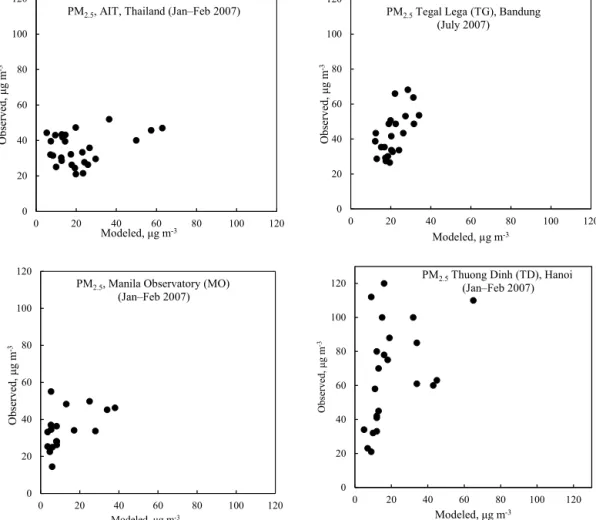
avail-able in the domain in 2007 for the model evaluation (Fig. 4). This study used the 24 h PM2.5 data monitored in the SEA

cities of Bandung, Bangkok, Hanoi, and Manila, under the AIRPET project (Kim Oanh et al., 2006, 2014). The obser-vation data were only available for some specific periods in 2007 at different sites and hence the modeled results were extracted for the corresponding periods for comparison. The observed sites were the mixed sites which were influenced by typical emission sources in the respective cities. The AIT site, located about 650 m away from a heavily traveled road, represented a suburban site with the influences of emissions from traffic and OB of rice straw (Kim Oanh et al., 2009). Thuong Dinh (TD) of Hanoi was a mixed urban site in-fluenced by traffic and residential combustion among other sources (Hai and Kim Oanh, 2013). Both Tegalega (TG), lo-cated in Bandung, Indonesia, and Manila observatory (MO)

0 10 20 30 40 50 60

January February March August September October

Concen

tratio

n,

µg m

-3

PM10, Kuala Lumpur, Malaysia (1 station)

Modeled Observed 0 20 40 60 80 100 0 20 40 60 80 100 Ob served, µg m -3 Modeled, µg m-3

PM10, Kuala lumpur, Malaysia

0 20 40 60 80 100 0 20 40 60 80 100 Ob served, μ g m -3 Modeled, µg m-3 PM10, Surabaya, Indonesia 0 10 20 30 40 50 60

January February March August September October

Concen

tratio

n,

µg m

-3

PM10, Surabaya, Indonesia (1 station)

Modeled Observed 0 20 40 60 80 100 0 20 40 60 80 100 Ob served, μ g m -3 Modeled, µg m-3 PM10, Bangkok, Thailand 0 10 20 30 40 50 60 70 80

January February March August September October

Concen

tratio

n,

µg m

-3

PM10, Bangkok, Thailand (2 stations)

Modeled Observed

Figure 3. Comparison of modeled and observed 24 h PM10in Kuala Lumpur, Malaysia (one station), Surabaya, Indonesia (one station), and

Bangkok, Thailand (three stations). Note that the stations included in the comparison are those located within the cell.

in Manila, Philippines, were mixed urban sites with strong influence of traffic and other typical urban sources. The data therefore represent different periods of the year and different urban characteristic sites and are only for model performance evaluation, not to compare the levels between the cities.

Overall, the available observed 24 PM2.5data in four

AIR-PET cities ranged from 4 to 120 µg m−3while the modeled values for the same data periods ranged from 5 to 64 µg m−3. The average levels of the observed PM2.5over all the data

pe-riods ranged from 35 to 43 µg m−3as compared to the

mod-eled, i.e., from 9.7 to 21 µ gm−3. Scatter plots of observed and modeled 24 h PM2.5 at four AIRPET stations (Fig. 4)

clearly showed that the model underestimated 24 h PM2.5

in all stations. In the mixed polluted urban site in Ban-dung (TG), modeled 24 h PM2.5 were within the range of

11–33 µg m−3while the observed were 27–69 µg m−3. In the TD urban site in Hanoi (close to a busy road), the simulated 24 h PM2.5were 5–64 µg m−3as compared to the observed of

20–120 µg m−3. In the mixed urban site of MO in Manila the simulated 24 h PM2.5 were 6–37 µg m−3 as compared to the

2736 D. A. Permadi et al.: Modeling PM and BC distributions in Southeast Asia 0 20 40 60 80 100 120 0 20 40 60 80 100 120 Ob served, μ g m -3 Modeled, μg m-3

PM , AIT, Thailand (Jan–Feb 2007)2.5

0 20 40 60 80 100 120 0 20 40 60 80 100 120 O bs er ve d, μ g m -3 Modeled, µg m-3

PM2.5Tegal Lega (TG), Bandung

(July 2007) 0 20 40 60 80 100 120 0 20 40 60 80 100 120 Ob served, μ g m -3 Modeled, μg m-3

PM , Manila Observatory (MO)2.5

(Jan–Feb 2007) 0 20 40 60 80 100 120 0 20 40 60 80 100 120 O bs er ve d, μ g m -3 Modeled, μg m-3

PM2.5Thuong Dinh (TD), Hanoi

(Jan–Feb 2007)

Figure 4. Scatter plots of modeled vs. observed 24 h PM2.5at four AIRPET sites, 2007.

Table 4. Statistical parameters for CHIMERE model performance (PM10and BC) evaluation.

Parameters and station name Statistical measures MBE MFB MFE (µg m−3) (%) (%) PM10a

1. BMR (average of 10 and 11 T)b −17.5 −53.3 55.7 2. SUF1 (Surabaya)c −2.6 −8.9 18 3. Jerantut, Kuala Lumpurd −13.6 −56.3 66.5 4. Petaling Jaya, Kuala Lumpure −10.3 −41.1 56.1 BCf

AIT site −0.12 −3.3 20.8 Note: criteria from Boylan and Russel (2006). MFB: PM ≤ ±60 %. MFE: PM ≤ +75 %; all the parameters satisfy the criteria of MFB and MFE. No criteria are available for MBE.

a_{Period taken was from January to March and August to October 2007 for all stations}

(daily average concentrations).

b_{Urban mixed site.} c_{Urban mixed site.} d_{Background concentration.} e_{Urban mixed site.}

f_{Period taken was from March to December 2007 (daily average concentrations).}

observed range of 4–55 µg m−3. As discussed above, the four selected AIRPET sites were located quite close to heavily traveled roads (although they were not directly on the road-side) and hence the local traffic emissions could directly af-fect the monitored pollution levels. This may be an important reason for the discrepancy between the monitored levels and the simulated grid average values. In addition, the observed data points were quite limited for 2007 (≤ 30 at each site) and were thus not sufficient for the statistical model perfor-mance evaluation. The PM2.5 monitoring efforts should be

enhanced to characterize the pollution in SEA and also pro-vide sufficient data points for the model evaluation.

3.3.3 Black carbon

For model evaluation purposes, we used available measure-ments in the previous projects for SEA. The 24 h BC mea-sured by the optical method was available at several SEA sites under the AIRPET project (Kim Oanh et al., 2014). The hourly-based EC (elemental carbon, measured by a Sun-set analyzer) measurements, available from the APN project (Kondo et al., 2009) for the AIT site (suburban), were used to

0 2 4 6 8 10 0 2 4 6 8 10 Ob served, µg m -3 Modeled, µg m-3 24 h BC, AIT, Thailand 0 2 4 6 8 10 12 BC, µg m-3 Julian days, 2007

24 h BC at AIT site (Thailand) Modeled

Observed

Figure 5. Time series comparison and scatter plot of modeled vs. observed 24 h elemental carbon in AIT site, 2007.

calculate 24 h BC levels. EC was measured using thermal op-tical method while BC was measured using light absorption method (continuous soot monitoring system or COSMOS). The model performance evaluation was done using 24 h BC data of both APN and AIRPET projects.

The APN hourly EC dataset for the AIT site was available for both dry and wet seasons, from March to December 2007. The hourly EC and hourly BC measured simultaneously by the APN project at AIT were found to have a strong linear correlation (Kim Oanh et al., 2009). Therefore, we used the observed Sunset EC to compare with the modeled output of BC. This is because for the PM mass closure, EC seems to be better while BC is suitable for radiative transfer budget analysis (Gelencsér, 2004). Figure 5 presents the time series of the modeled and observed 24 h BC for the AIT site. The modeled 24 h BC was from 1.0 to 10 µg m−3that is compara-ble with the observed range from 0.8 to 10 µg m−3. However, correlation between the modeled and observed BC shown in the scatter plot was fairly low. The discrepancy between the modeled and observed BC seen in the time series may principally be due to the gridded average of the model

out-put as compared to the point-based measurement. Higher BC levels measured at the AIT site were contributed by mul-tiple local sources, such as nearby highway traffic activity and biomass OB (of rice straw) that occurred more inten-sively during the dry season (December). However, these sources, especially small-scale rice straw field burning ac-tivity, may not be well represented spatially by the EI input data made for a large resolution (30 km × 30 km). Three sta-tistical measures of MBE, MFB, and MFE were considered for the model performance evaluation in the BC simulation at the AIT site (Table 4). The MFB and MFE values were −24 and 49 %, respectively, which meet the suggested crite-ria (for PM). The MBE value was −0.12 µg m−3for the AIT site, which showed that the model somewhat underestimated the observed BC values, but there are no MBE criteria avail-able for PM for comparison.

The 24 h BC (optically) measured on the 24 h PM2.5

sam-pled filters collected in the same locations of PM2.5

measure-ments in SEA under the AIRPET project (Kim Oanh et al., 2006, 2014) were compared with the 24 h modeled BC ex-tracted for the sites and dates of 2007. Figure 6 shows that

2738 D. A. Permadi et al.: Modeling PM and BC distributions in Southeast Asia R² = 0.1535 0 2 4 6 8 10 12 0 2 4 6 8 10 12 Ob served, μ g m -3 Modeled, μg m-3 24 h BC, AIT (Jan–Feb 2007) 0 2 4 6 8 10 12 0 2 4 6 8 10 12 Ob served, μ g m -3 Modeled, µg m-3 24 h BC, TG, Bandung (July 2007) 0 5 10 15 20 25 0 5 10 15 20 25 Ob served, μ g m -3 Modeled, μg m-3 24 h BC, MO (Jan–Feb 2007

)

Figure 6. Comparison of 24 h simulated and observed BC at four AIRPET sites in SEA domain, 2007.

the modeled 24 h BC were lower than the observed at all the sites. The ranges of observed values and modeled values were in somewhat better agreement for the AIT site and MO site than the other two sites. At AIT, the observed BC val-ues were 1.3–3.4 µg m−3(January, February, and May) were higher but quite comparable to the modeled range of 0.5– 1.8 µg m−3. At MO, the observed 24 h BC of 7–13 µg m−3 (January and February) was quite close to the modeled 24 h BC of 4.2–13 µg m−3. More discrepancies were found for the Bandung site, with observed 24 h BC values ranging from 4.2 to 9.8 µg m−3(July 2007) as compared to the modeled val-ues of 1.3–3.2 µg m−3. Similarly, the observed BC values at the mixed site of TD, Hanoi, ranged from 12 to 23 µg m−3 (January 2007), much higher than the modeled values of 1–7 µg m−3. The effects of local sources, especially traffic emissions, at the quoted sites should be a main cause of the discrepancies when compared to the grid average mod-eled BC with the observed values. The limited measurement data available prevented a more comprehensive model per-formance evaluation. Note that due to the limited

measure-ment data points, a statistical performance evaluation was not conducted for the BC simulation.

3.3.4 Ratios between fine and coarse PM and between BC and PM

In fact, PM2.5 mass is principally contributed by both

lo-cal combustion sources and secondary particles formation by chemical reactions in the atmosphere. The gaseous pre-cursors of NOx, SOx, and VOCs for the PM2.5 formation

may be of both local and LRT origins. The coarse fraction

(PM10−2.5) would mainly consist of primary particles of the

geological origin (Chow et al., 1998), and these are mainly contributed by local sources of soil, road dust, and construc-tion activities (Hai and Kim Oanh, 2013). Due to its for-mation process as well as the ability to participate in the regional transportation, the fine particles (PM2.5) are more

uniformly distributed in an urban area than the coarser par-ticles. The PM2.5/PM10ratios could provide some

com-pare the PM2.5/PM10ratios based on the modeled 24 h PM2.5

and 24 h PM10(PM10=PM2.5+PM10−2.5) with those

com-puted from the observed PM data available at the four AIR-PET monitoring sites discussed above. Overall, the modeled PM2.5/PM10 ratios ranged from 0.47 to 0.59 while the

ob-served values were higher, 0.6–0.83. More pronounced dif-ferences were for TD, i.e., 0.74 observed vs. 0.47 modeled, and for TG of Bandung, 0.83 observed vs. 0.55 modeled. Better agreements were obtained for MO, 0.61 observed vs. 0.47 modeled, and the AIT site, 0.60 observed vs. 0.59 mod-eled. The urban mixed sites of TD in Hanoi and TG in Bandung were located in the traffic areas and thus higher contributions of the primary PM2.5 emitted from traffic to

the total measured PM10 may be seen compared to the MO

and AIT sites. However, to evaluate the variations in the PM2.5/PM10 ratios, contributions of various sources of the

coarse particles, such as road dust and construction dust, should be further analyzed. It is noted that the ratios used to compare with the model-simulated values were all de-rived from the observations made in large cities in SEA. Lack of observation data in rural areas and remote sites presents an obstacle for more in-depth analysis of the model per-formance. The remote sites, with less influence of the local sources, could be valuable for the model performance evalu-ation, both for the PM mass concentrations and their ratios.

BC is emitted directly from the combustion sources with higher fractions in PM emitted from the diesel exhaust (Kim Oanh et al., 2010) and lower fractions from biomass OB (Kim Oanh et al., 2011). Hence the ratio of BC/PM2.5,

for example, can infer the contribution of the primary particles from these combustion activities. BC/PM2.5 and

BC/PM10ratios were calculated using the observed 24 h data

at four AIRPET sites. Modeled BC/PM2.5ratios ranged from

0.05 to 0.33 as compared to the observed ratios of 0.05–0.28. For BC/PM10, the modeled values ranged from 0.03 to 0.16

while the observed values ranged from 0.034 to 0.17. Ob-served BC/PM2.5 ratios were higher than the modeled

val-ues at TG of Bandung (0.16 vs. 0.1) and AIT (0.055 vs. 0.05) sites. In TD and MO, the observed ratios (0.22 and 0.23) were lower than the modeled (0.28 and 0.33). As for BC/PM10,

the observed ratios at three AIRPET sites of TG, TD, and AIT (0.13, 0.17, and 0.034) were higher than the modeled values (0.06, 0.13, and 0.03), while for MO the opposite was shown with a lower observed (0.14) as compared to the mod-eled (0.16) value. The simulated BC/PM ratio was the high-est in TD, 0.22 % for PM2.5and 0.17 % for PM10, during the

dry period of January–February 2007, which confirmed the strong influence of traffic emission at this site.

The lack of data for the areas outside the cities is a remain-ing issue. Generally, we expect that PM2.5mass may be more

uniform in an urban area; for example, measurements con-ducted in several mountain areas in Asia showed high PM2.5

concentrations which were mainly due to the regional trans-port (Hang and Kim Oanh, 2014; Co et al., 2014) or local combustion sources (e.g., residential cooking, biomass OB)

such as found in China (Liu et al., 2017). However, the BC fraction of PM may vary a lot with much lower values in remote sites but a lack of data prevents a more in-depth anal-ysis.

As seen in the statistical model evaluation, a negative MBE was obtained for PM10, −3 to −17, and BC, −0.12, at all

sites (not enough data for statistical evaluation of PM2.5),

which showed an underestimation of PM10 and BC

concen-trations by the model at the sites. This may be explained by the coarse resolution (30 km × 30 km) of emission input data which could not adequately represent the spatial dis-tributions of local sources on a smaller scale, such as road traffic. These local sources, for example road traffic and res-idential cooking, affect PM measured at all sites, hence af-fecting the PM2.5/PM10 and BC/PM ratios. The road and

soil dust emissions contribute more to PM10−2.5, thus

lower-ing PM2.5/PM10 ratios in urban areas, but this coarse

frac-tion of PM emission was not included in our emission in-put file. In addition, the LRT pollution above the model top layer (> 500 hPa) may contribute to the pollution in the do-main, more to PM2.5 and BC than the coarse PM. The

free-tropospheric LRT of aerosol and high convective processes should be also considered by extending the vertical model setup in future studies.

3.4 Spatial distribution of modeled monthly PM10,

PM2.5, and BC

Spatial distributions of the modeled monthly average PM10,

PM2.5, and BC are presented in Fig. 7 for January,

Au-gust, and November while those of the respective annual averages are presented in Fig. S7 in the Supplement. The highest monthly average concentrations of PM10 in

Jan-uary, August, and November 2007 simulated in the do-main (one value for the whole dodo-main) were 69, 58, and 44 µg m−3 while corresponding values of PM2.5 were 40,

37, and 27 µg m−3, respectively. The simulated maximum monthly average BC concentration in the domain was higher in January (8.2 µg m−3) as compared to August (7.8 µg m−3) and November (5.9 µg m−3).

The simulated highest hourly PM10values in the

consid-ered months of January, August, and November 2007 were 325, 245, and 164 µg m−3, respectively, while the PM2.5

cor-responding values were 188, 150, and 99 µg m−3. The highest values of simulated annual average in the domain for PM10

and PM2.5 were 51 and 32 µg m−3, respectively. The

max-imum simulated annual average in the domain for BC was 6 µg m−3. A summary of the simulated pollutant levels in the domain is presented in Table S3 in the Supplement.

For all considered pollutants over the domain, higher con-centrations were observed over East Java, Indonesia, par-ticularly over Surabaya, which shows the effects of emis-sion from residential and traffic in the city and surrounding satellite cities as well as the crop residue OB (Permadi and Kim Oanh, 2013; Permadi et al., 2017b). High concentrations

2740 D. A. Permadi et al.: Modeling PM and BC distributions in Southeast Asia

Figure 7. Spatial distribution of monthly average PM10, PM2.5, and BC in the selected months, 2007.

were consistently observed in several places in Indonesia in-cluding Java, West Sumatra (Padang), and West Kalimantan (Pontianak) and over Bangkok, Thailand. Large hotspots but with lower concentrations were also observed over Southern China and over Hanoi and Ho Chi Minh (Vietnam), which can be largely explained by the influence of the local sources (Fig. 7).

The monsoon circulation plays an important role in trans-porting PM from the emission source regions to other parts of the domain. In the dry months, higher emissions of biomass OB are expected, and higher concentrations of PM should be seen in the region near and downwind of sources. Ac-cordingly, in the northern part of the domain, higher PM lev-els were found in January–April, while in the southern part of the domain higher concentrations were found during the period of April–August. In January in the Northern Hemi-sphere, the Northeast Monsoon transports pollutants from the source regions to the southwest, while in the Southern Hemisphere (Indonesia) the plume moved to the northeast– east. The opposite is seen in August and November (Fig. 7). In August in the Southern Hemisphere, the plumes of PM

moved northwesterly and turned northeasterly after reaching the Equator line. The plumes of PM10and PM2.5converged

in the South China Sea in January and November when the Northeast Monsoon was prevalent that brought PM pollution from the southern part of mainland China to the South China Sea (Figs. S8a–d). WRF results showed no rainfall over the South China Sea during the particular period, which may also contribute to the high PM levels in the converged zone (Figs. S8e–f).

In August and November, the dry months in the southern domain, the PM10and PM2.5plumes showing the effects of

biomass OB (crop residue and forest fire) emissions in In-donesia that originated in Riau province (Sumatra) and west-ern and southwest-ern parts of Borneo were seen clearly moving northeastward. In January, the dry season month in the north-ern domain, the plumes of PM10 and PM2.5 intensified by

biomass OB in the central and northern parts of Thailand were shown moving southwestward. BC plumes generally originated from big cities in the domain, showing a signif-icant influence of fossil fuel combustion emissions, specif-ically from traffic and other urban activities for all months

of the year. During the dry period, BC plumes from the areas that have intensive biomass OB emissions were not as clearly seen as the PM plumes and this may be because biomass OB contributed more to OC than BC emissions.

Effects of precipitation on the PM levels were also seen; e.g., higher PM levels (Fig. 7) were simulated over Indochina in January, October, and November as compared to August because the latter was a rainy month in this part of the do-main, i.e., less biomass OB and more wet removal in prin-ciple. The opposite was actually seen in the southern part of modeling domain, e.g., above Indonesia, where lower PM levels were simulated in October (rainier month in this part) than other months.

3.5 Aerosol optical depth

Both total AOD and BC AOD were considered for the model evaluation. The monthly average of the total columnar AOD (scattering and absorbing), at the wavelength of 550 nm, was produced from the AODEM simulation for 2007. The simu-lated monthly AOD data were compared with the monthly Terra MODIS AOD, also at 550 nm, retrieved from the NASA website. Figure 8 showed that the modeled AOD was lower than the MODIS observed; for example in January, the maximum AOD simulated for the Southern China part of the domain was about 0.36 as compared to the MODIS AOD of 0.42–0.58. In the same month, the modeled AOD val-ues over Java, Indonesia, were 0.072–0.28 while the MODIS AOD values were 0.26–0.42. In April, the model results over Southern China were 0.25–0.75 while the observed MODIS AOD was 0.42–0.90. Near the border between Myanmar and Bangladesh (northwest corner of the domain), the modeled AOD and the observed MODIS AOD were similar, 0.74– 0.75. However, the modeled AOD values over Java in April were higher, i.e., 0.02–1.0, than the observed MODIS AOD of 0.26–0.42. The simulated hourly maximum and monthly average PM10 and PM2.5 concentrations, and hence AOD,

over Java were the highest throughout the year. In particular in April, there was a hotspot of AOD simulated over the lo-cation that may be due to the meteorological conditions. For example, the restricted dispersion conditions in April could be seen from the smaller dispersion plumes in this month as compared to other months in Fig. 8.

In October, a hotspot with the maximum AOD of 0.8 was observed by MODIS over Riau, Sumatra, and Singapore that was well above the model result for the grid of 0.4. The model was also not able to capture AOD hotspots over main-land Southern China in this month. The results for August and November both showed some significant underestima-tion of AOD as compared to the MODIS-observed values. There are several reasons for these discrepancies, including the temporal and spatial inconsistency in the observed and modeled values used for comparison. For example, the Terra MODIS satellite daily passed a region for a particular time (i.e., 13:30), thus giving only a snapshot of the value, while

(a) Modeled AOD (b) MODIS AOD

October January April November August October November August April January

Figure 8. Spatial distribution of monthly modeled AOD as com-pared to the MODIS Terra AOD for the selected months, 2007.

the model provided the hourly average for 13:00–14:00. Thus there is certainly inconsistency in the monthly averages de-rived from these two datasets. The discrepancy may come from the fact that in the simulation AOD was covering up to 500 hPa and could not include aerosol in the upper layers as mentioned above. Different spatial resolutions of modeled AOD (30 km×30 km) and MODIS AOD (10 km×10 km) can be another reason. In addition, shipping emissions and the natural sources of aerosol, such as wind-blown dust, were not included in our emission input data so the model would pro-duce lower AOD (as well as PM10) values. Consistent with