The Fall in Income Inequality during COVID-19 in Five European Countries

(1)

HAL Id: halshs-03185534

https://halshs.archives-ouvertes.fr/halshs-03185534

Preprint submitted on 30 Mar 2021

HAL is a multi-disciplinary open access archive for the deposit and dissemination of sci-entific research documents, whether they are pub-lished or not. The documents may come from teaching and research institutions in France or abroad, or from public or private research centers.

L’archive ouverte pluridisciplinaire HAL, est destinée au dépôt et à la diffusion de documents scientifiques de niveau recherche, publiés ou non, émanant des établissements d’enseignement et de recherche français ou étrangers, des laboratoires publics ou privés.

The Fall in Income Inequality during COVID-19 in Five

European Countries

Andrew Clark, Conchita d’Ambrosio, Anthony Lepinteur

To cite this version:

Andrew Clark, Conchita d’Ambrosio, Anthony Lepinteur. The Fall in Income Inequality during COVID-19 in Five European Countries. 2021. �halshs-03185534�

(2)

WORKING PAPER N° 2021 – 21

Life Satisfaction and the Human

Development Index Across the World

Andrew E. Clark Conchita D’Ambrosio

Anthony Lepinteur

JEL Codes: D63, I32, I38.

(3)

The Fall in Income Inequality during

COVID-19 in Five European Countries

*

A

NDREW

E. C

LARK

Paris School of Economics - CNRS

andrew.clark@ens.fr

C

ONCHITA

D’A

MBROSIO

University of Luxembourg

conchita.dambrosio@uni.lu

A

NTHONY

L

EPINTEUR

University of Luxembourg

anthony.lepinteur@uni.lu

This version: March 2021

Abstract

We here use panel data from the COME-HERE survey to track income inequality during COVID-19 in France, Germany, Italy, Spain and Sweden. Relative inequality in equivalent household disposable income among individuals changed in a hump-shaped way over 2020. An initial rise from January to May was more than reversed by September. Absolute inequality also fell over this period. As such, policy responses may have been of more benefit for the poorer than for the richer.

Keywords: COME-HERE, COVID-19, Income Inequality. JEL Classification Codes: D63, I32, I38.

* We would like to thank Thomas Blanchet, Liyousew Borga, Walter Bossert, Giorgia Menta, Vincent Vergnat and Remi Yin for their help and feedback. We also thank the Editor, Andreas Peichl, and two anonymous referees for comments that helped improve the paper. Financial support from the André Losch Fondation, Art2Cure, Cargolux, and the Fonds National de la Recherche Luxembourg (Grant 14840950 – COME-HERE) is gratefully acknowledged. Andrew Clark acknowledges financial support from the EUR grant ANR-17-EURE-0001.

(4)

1

1. Introduction

At the time of writing, over 125,000,000 cases of COVID-19 have been reported globally, and the number of new infections in some Western European countries like France, Germany, Italy, Sweden and Spain is not decreasing. In line with epidemiological models (Ferguson et

al., 2020, and Lourenco et al., 2020), many governments have adopted policies aiming to

restrict population movement (such as lockdowns, travel restrictions and curfews). The rationale for these restrictions is to save lives and prevent health systems from being overwhelmed. These policies have produced unprecedented effects on household incomes, which Governments have addressed via extraordinary measures such as furlough payments and direct support of those who lost the most during the pandemic. While much of this effort has been national, in Europe the European Union recently agreed to complement national programmes via the largest-ever stimulus package of €1.8 Trillion to help rebuild a greener, more-digital and more-resilient post-COVID-19 Europe.

There is a very fast-growing literature on the impact of COVID-19 lockdowns (some examples are Brodeur et al., 2021, Layard et al., 2020, and Fang et al. 2020), and more generally the economic and distributional consequences of the COVID-19 pandemic. Our aim here is to track household disposable-income inequality during the COVID-19 period using direct information from surveys on income.

We have access to a unique longitudinal high-frequency information on household disposable income in five European countries (France, Germany, Italy, Spain and Sweden) from the COME-HERE survey run by the University of Luxembourg since the end of April 2020. COME-HERE allows us to track relative and absolute inequality in equivalent disposable household income among individuals between January, our pre-COVID-19 observation, and September 2020. While the five countries in our analysis are comparable in terms of economic development, they are not so regarding the spread of COVID-19 and pandemic policy

(5)

2

responses. Our sample includes both Italy, the first country to introduce a national lockdown on March 9th_{2020, and Sweden, which never had a lockdown in 2020.}

In line with most micro-simulation results (Almeida et al., 2020, Brewer and Tasseva, 2020, O’Donoghue et al., 2020, Li et al., 2020, Brunori et al., 2020), relative inequality in most of our five countries fell between January and September 2020: one by-product of government compensation schemes has been to reduce relative inequality. The exception is France, with a slight increase in relative inequality as measured by half the square of the Coefficient of Variation (GE(2)) coming from wider income differences at the top of the distribution. The same country pattern is found in indices of absolute inequality (measuring the gaps in income levels, as opposed to shares).

The decomposition of these changes in relative inequality by age, gender, education and marital status, reveals that most movement has been within groups; the between-group changes are mixed.

The remainder of the paper is structured as follows. Section 2 reviews the literature on the effect of the COVID-19 pandemic on income changes and inequality, and Section 3 describes the COME-HERE survey and the measures of inequality we use. Section 4 then presents our results regarding the evolution of income inequality in France, Germany, Italy, Spain and Sweden between January and September 2020. Section 5 presents a number of robustness checks, and Section 6 concludes.

2. Literature Review

The COVID-19 pandemic has had substantial effects on individual outcomes. Some of the related work has explicitly focused on the labour market. Adams-Prassl et al. (2020) show that the pandemic in March and April 2020 had a negative impact on labour-force participation (LFP) and working time: these effects were stronger in the UK and the US than in Germany, and, within countries, hit less-educated workers and women harder, and so exacerbated

(6)

pre-3

existing inequality. Using US data from the American Time Use Survey in 2017 and 2018, Alon et al. (2020) predict that the COVID-19 shock will increase gender inequality by placing a disproportionate burden on women. Compared to past recessions, the fall in employment due to social distancing had a greater effect on sectors with high female-employment rates; at the same time, women have shouldered the lion’s share of the burden of greater childcare following the closure of schools and daycare centres. Using Spanish data, Farré et al. (2020) come to similar conclusions. Exploiting variations across US States in COVID-19 cases and death, Beland et al. (2020)show that COVID-19 increased unemployment, reduced hours of work and LFP, but had no significant effect on wages: these detrimental effects were more pronounced for some types of workers (e.g., Hispanic and younger workers). Similar conclusions are reached by Guven et al. (2020), using the Longitudinal Labour Force Survey data up to the end of May 2020 in Australia: COVID-19 reduced LFP by 2.1%, increased unemployment by 1.1% and produced a one-hour drop in weekly working hours. The effect again differed across groups, with the LFP and working hours of the less-educated being more affected, and unemployment rising more for immigrants and those with shorter job tenure or occupations unsuitable for remote work. Bottan et al. (2020) equally underline the greater impact of COVID-19 on the least well-off in Latin America and the Caribbean between January and April 2020 using online-survey data.

Bonacini et al. (2021) simulate the feasibility of working from home using data on worker characteristics in Italian surveys from 2013 and 2018. Working from home is suggested to be easier for male, older, better-educated and higher-paid workers, increasing labour-income inequality. The four hypothetical scenarios of stringent policy response across 29 European countries in Palomino et al. (2020) also produce uneven wage losses and rising wage inequality.

(7)

4

The above contributions covered the labour market; we here wish to focus on household disposable income, of which labour income is only one (important) part. Beyond direct labour-market intervention, Governments have also implemented a variety of other policies, such as mortgage holidays, rent support, and fiscal, monetary and macro-financial policies. The policy tracker of the IMF contains an excellent, and regularly updated, summary of the key economic responses of the governments of 197 countries (see https://www.imf.org/en/Topics/imf-and-covid19/Policy-Responses-to-COVID-19).

Two broad approaches have been taken to track household disposable-income inequality during COVID-19. The first appeals to micro-simulation and calibration, due to the scarcity of adequate recent micro data. Using EUROMOD, Almeida et al. (2020) simulate separately the effect of the pandemic and the subsequent policy responses in 27 European countries. In the absence of policy response, the 2020 relative Gini coefficient would have risen by 3.6 percent, but following the policy response relative inequality instead fell by 0.7 percent. Brewer and Tasseva (2020) reach the same conclusion using the UK module of EUROMOD, with lower values of the Gini coefficient, Theil index and Mean Logarithmic Deviation in 2020 from the COVID-19 policy responses and the pre-existing tax-benefits system; see also O’Donoghue et

al. (2020) and Li et al. (2020) for Ireland and Australia, respectively. Brunori et al. (2020)

simulate the short-term effects of two months of lockdown on Italian income distribution in the IRPET MicroReg tax model. Again, the Gini coefficient for equivalent disposable household income falls due to policy interventions that target the poorest, from 0.3396 to 0.3373. However, the Italian analysis using EUROMOD in Figari and Fiorio (2020) predicts rising inequality from one month of lockdown.

The second approach to income inequality uses direct information from surveys on income changes. This data is scarcer, and is often cross-sectional and of relatively-low frequency. Brewer and Gardiner (2020) suggest that the probability of reporting lower household income

(8)

5

was relatively constant across pre-COVID-19 income quintiles in a cross-section of 6,000 UK adults in early May 2020. Belot et al. (2020) use cross-section data from China, Japan, South Korea, Italy, the UK and the US in April 2020 (around 1,000 respondents per country) to show that those aged 18-25 were more likely to experience a drop in household income. Neither of these papers calculates formal inequality indices.

The scarcity of data of this nature, let alone longitudinal and cross-country, is understandable given the cost and associated challenges. As Figari and Fiorio (2020, p.2) note: “Lack of longitudinal up-to-date information on household income and labour market

circumstances, usually available a few years after the economic shock and in a limited number of countries only, constrains the possibilities for empirical analysis”. Our use of recent,

high-frequency cross-country panel data helps to fill this gap.

3. Data and Method

The data we use here are from the COME-HERE (COVID-19, MEntal HEalth, REsilience and Self-regulation) panel survey collected by the University of Luxembourg. The survey was conducted by Qualtrics in France, Germany, Italy, Spain and Sweden. Respondents complete an on-line questionnaire that takes approximately 20 minutes. Qualtrics runs specialised recruitment campaigns via its partner network, and is able to contact groups that may be hard to reach on the internet (older respondents, for example). Qualtrics uses stratified sampling, and the COME-HERE samples are nationally-representative in terms of age, gender and region of residence. Qualtrics also has data-quality protocols: for instance, the information supplied by respondents who answer the questionnaire in under ½ of the median survey-completion time is not retained, and a replacement interview is conducted. In the same spirit, the IP addresses of the respondents are checked and digital-fingerprinting technology is used to ensure that observations are not duplicated. Ethics approval for our study was granted by the Ethics Review Panel of the University of Luxembourg. The COME-HERE dataset collects information at the

(9)

6

individual and household levels, and is longitudinal. The first four waves of survey, which provide the data analysed here, were conducted around May 1st_{, June 9}th_{, September 5}th_and

November 20th 2020. The fifth wave was in the field in March 2021. At least three more waves are planned for 2021.

Over 8,000 individuals took part in the first survey wave, and were then invited to respond in subsequent waves (there have been no refreshment samples, given the satisfactory response rates). Around 82.5% took part in at least one other survey wave, with 42% participating in all four waves, 25% in three waves, and 15.8% in two waves. Our analysis will be carried out on unbalanced panel data. We show in the robustness checks that our conclusions are not sensitive to the use of a balanced panel or sample weights that guarantee national representativeness.

The objective of the survey is not only to collect sufficient individual information to describe living and mental-health conditions during COVID-19, but also to identify recent changes and events that might have affected individuals’ lives. Standard sociodemographic characteristics such as age, gender, education, and labour-force and marital statuses were also collected. Special survey modules in some waves addressed topics such as risk attitudes, time discounting, preferences for redistribution, income comparisons, and working conditions.

We measure income inequality via a question in each survey wave asking respondents about their household disposable income two to four months prior to the survey, with responses in the following bands: “0 to 1250 Euros”, “1250 to 2000 Euros”, “2000 to 4000 Euros”, “4000

to 6000 Euros”, “6000 to 8000 Euros”, “8000 to 12500 Euros” and “Over 12500 Euros”. Our

empirical analysis will cover household disposable income at three points in time. The first is January 2020 (reported in Wave 1), that we will take as the pre-COVID-19 figure. The second refers to May 2020 (from Wave 3), at the end of the first COVID-19 wave and the third to September 2020 (from Wave 4), after the Summer but before the beginning of the second wave

(10)

7

of COVID-19 in Europe. The income question in Wave 2 adds little information as it refers to April, producing very similar figures to those for May in Wave 3.

To track the evolution of income inequality across Europe, we first estimate Lorenz curves and calculate four relative measures of inequality: Gini, and three members of the Generalized Entropy family - Mean Logarithmic Deviation (GE(0)), Theil (GE(1)) and half the square of the Coefficient of Variation (GE(2)). These indices differ in their sensitivity to income changes, with the Gini coefficient being more sensitive to income differences around the mode of the distribution, and Generalized Entropy measures increasingly to changes affecting the upper tail as the parameter values in parentheses rise from 0 to 2.

The Generalized Entropy measures are the only Lorenz-consistent indices that are additively decomposable by population subgroups. We make use of this property in the next section to see if some groups were more affected than others, and decompose relative inequality within and between age, gender, education and marital status.

The scale-invariance property of the Lorenz-consistent measures implies that inequality remains unchanged as all incomes change in the same proportion: we measure inequality in income shares. This is not the only way forward, and departures from the relative criterion have become increasingly common following the finding in Atkinson and Brandolini (2004) that the evolution of world income inequality differed with relative and absolute measures. We thus turn to absolute measures of inequality. The translation-invariance property of these indices imply that now inequality is unchanged as all incomes change by the same amount: we measure inequality in levels of income. We will here consider the absolute Gini coefficient, the variance of the income distribution, and two versions of the Kolm index with inequality-aversion parameters of 5*10-4 and 10-4 (the results are very similar with other parameter values).

Our empirical analysis covers all respondents with valid information on disposable household income. As this latter is measured in bands, we take the mid-point in Euros and in

(11)

8

PPP (using 2019 Euros for household final consumption expenditures as the reference). We attributed a value of 12 500 Euros to the open-ended top income category: this value produces the best fit when comparing our relative Gini coefficients in January 2020 to those produced by Eurostat in 2019. Each income figure is then equivalized using the square root of the number of household members, and the resulting value is then attributed to each household member. The decomposition by population subgroups is carried out taking as reference the characteristics of the survey respondent.

There are 17,183 observations (7,302 individuals) in the analysis sample. The French, German, Italian and Spanish samples cover around 22% of the sample each, but the Swedes only 11% of observations, in line with the countries’ relative populations.

It is natural to compare COME-HERE to the benchmark dataset used in Europe to monitor poverty and inequality, EU-SILC. The latter is a collective enterprise at the European Union level by National Statistical Institutes under the coordination of EUROSTAT with immense expertise in data collection and production. COME-HERE is not on the same scale as EU-SILC, but has the great advantage of already being available and offering multiple observations over 2020, which are fundamental qualities for the monitoring of inequality during the pandemic. When we compare our relative Gini coefficients from January 2020 to the latest

figures produced by Eurostat, available at

https://ec.europa.eu/eurostat/databrowser/view/ilc_di12/default/table?lang=en, we find very similar values in France, Germany, Spain and Italy: the Eurostat Gini coefficients in 2019 were respectively 0.292, 0.297, 0.328 and 0.330, while the analogous COME-HERE figures from January 2020 were 0.294, 0.302, 0.336 and 0.339. None of these differences are therefore over 0.8 Gini points. The only exception is Sweden, where our Gini coefficient is higher than that from Eurostat: 0.314 versus 0.276. We also find that the average equivalised disposable household incomes in COME-HERE in France, Sweden and Germany in January 2020 are very

(12)

9

similar to those that can be calculated from the most recent EU-SILC wave (after applying the same equivalence scale and PPP indices). The picture is somewhat different in Spain and Italy, where the average COME-HERE equivalised disposable household incomes are roughly 20% lower than those in EU-SILC, so that we are missing some observations in the right tail of the income distributions. The similarities in terms of Gini coefficients between the two datasets are reassuring for the analysis of inequality. In addition, we are mainly interested in monitoring changes over time, so the values at baseline are somewhat less of a concern.

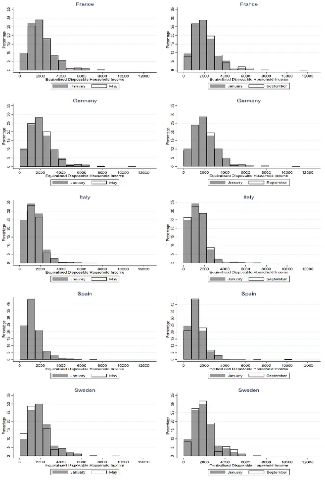
Before turning to the analysis of inequality in the next section, we first describe the observed changes in income densities with the summary statistics in Table 1 and the histograms in Figure 1. Average equivalised disposable household income across all countries is U-shaped from January to September 2020, falling by 3.2% between January and May and then recovering to almost its initial level by September. The initial income fall in May 2020 likely reflects the COVID-19 outbreak per se and the initial restrictive measures, and the subsequent recovery the governmental compensation schemes implemented throughout 2020. This U-shaped income pattern is found in all individual countries bar France, where income instead rose fairly steadily over the period (although all of the income changes here, over a short period, are necessarily only quite small).

Median income over this eight-month period is somewhat more stable: this did not change in France and Germany, and increased in Sweden only between May and September. The U-shaped pattern found for mean income is also apparent in median income in Italy and Spain. Notably, Italy is the only one of our five countries in which neither mean nor median income had recovered to its January level by September.

The country income distributions are plotted in Figure 1. The left-hand panel here refers to the January-May movements, and the right-hand panel to those between January and September. The income distribution shifted to the left between January and May in Italy, Spain

(13)

10

and Sweden, while there is a notable higher concentration in the middle-income categories in Germany. We observe the opposite pattern in France: the middle-income categories attract slightly fewer observations.

Turning to the January-September distributions, we see a general shift from the bottom of the distribution towards values in the middle. Italy is the exception, and is notably the only country where the percentage of respondents with an equivalent income (in PPP) under 750 Euros per month in September remained higher than that in January.

4. Changing Income Inequality

We first visually inspect the changes in relative inequality by plotting in Figure 2 the Lorenz curves for first the whole sample and then separately for each country between January and September 2020. There is a slight shift of the Lorenz curve towards the line of perfect equality in the whole sample. The weak Lorenz dominance here (as there is some overlap at the extremes) indicates that relative inequality fell in the whole sample. A formal quantitative measure of this shift is provided by the Gini coefficient (measuring the normalized area between the line of equality and the Lorenz curve) at the foot of the figures: for the whole sample this fell from 0.322 to 0.314 between January and September 2020.

There are somewhat similar relative inequality patterns in all countries in the remaining panels of Figure 2, although there is no Lorenz dominance in France and Italy as the curves cross. In France the September curve is above that of January for lower income shares and below it for higher income shares; in Italy we find the opposite shift.

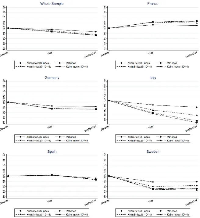
Figure 3 plots the Gini coefficient and the three Generalized Entropy indices in January, May and September 2020, where January is normalised to 100 as the baseline (the actual values with 90% confidence intervals appear in Appendix Table A1). In the top-left panel of Figure 3, for all countries together, all relative-inequality measures rose between January and May. For example, the Gini coefficient increased by roughly 0.6 points. We observe similar changes

(14)

11

in France, Spain, Italy and Sweden. These higher Gini coefficients are in line with the predictions made by Almeida et al. (2020) under the scenario of no policy intervention. Although some measures were already in place in May 2020, our results combined with those of Almeida et al. (2020) suggest that the policy responses to the COVID-19 emergency at that time were not immediately effective in tackling the rise in inequality. The higher Italian Gini coefficient is also very much in line with the simulations in Brunori et al. (2020) that compare pre-COVID-19 to a COVID-19 situation where the only governmental response is lockdown. Germany is an exception here: in May 2020, the Gini coefficient was lower (as indeed were all of the German inequality indices), so that the initial phase of the pandemic was associated with lower inequality.

The German experience at the beginning of the pandemic actually serves as a precursor for the four other countries in our sample as we move to September 2020: relative inequality is lower in September than in January in every country. The only exception is the GE(2) measure in France, where we see a slight increase due to greater income differences at the top of the distribution. The largest fall in relative inequality is found for the GE(2) in Italy and Sweden. In Italy, the fall in inequality depends on the Generalized Entropy parameter: the larger drop in GE(2) reflects the tightening of the income differences at the top of the distribution. We noted above the opposite shifts in the Lorenz curves in Italy and France, and these are consistent with their different GE(2) experiences.

The overall picture of the distribution of income in Europe during the pandemic can then be split into two periods. The advent of COVID-19 increased relative income inequality in the first period (except in Germany); however, in the second period the evolution of the pandemic and the effect of various policy interventions has more than reversed this initial widening of inequality.

(15)

12

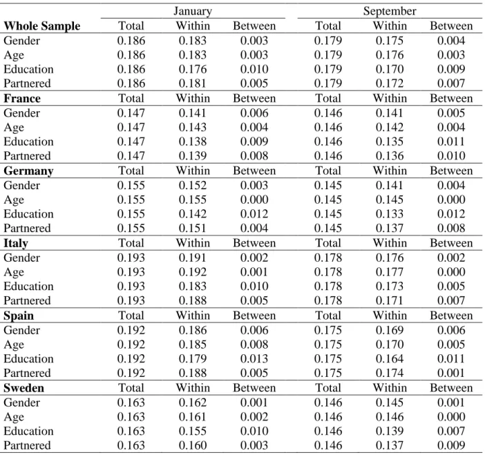
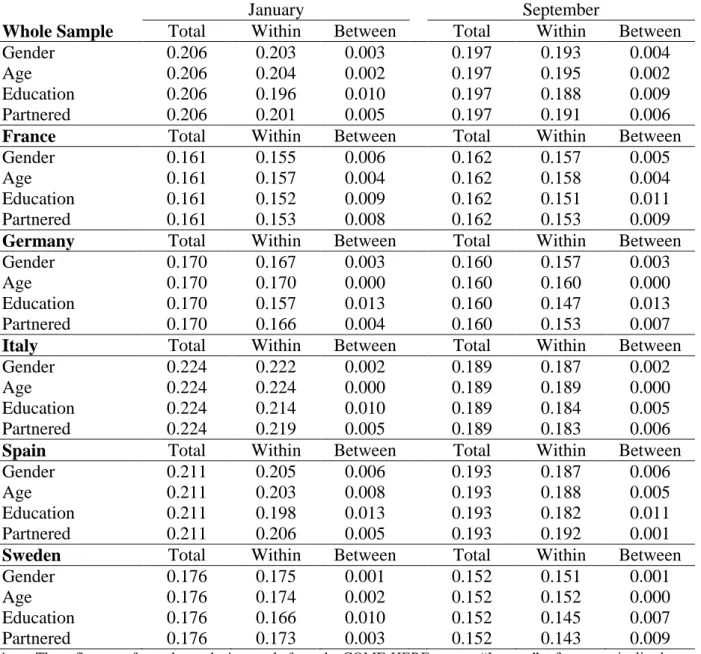
Tables 2 to 4 contain the decompositions of the three Generalized Entropy measures in January and September 2020 by four individual characteristics: gender, age (above/below 50), education (post-secondary education vs. otherwise) and being in a couple. First, in all countries and periods the within components explain by far the largest part of total inequality (both in levels and changes). This result is commonplace in the inequality literature.

We find that inequality within groups fell over time, with the exception of the GE(2) for the gender and age decompositions in France. That this is found only for GE(2), and not GE(1) and GE(0), highlights that the driver of increasing inequality within gender and age groups in France is the income changes in the upper tail of the distribution.

The results for the between group components are mixed, and for 24 out of the 52 country values there is no change. The largest change in the between component over time is with respect to education in France and Italy, and with respect to being in a couple in the other three countries. There is a drop in inequality between the weighted income means by education in all countries apart from Germany, where there is no change, and France, where this figure rises. We also find an increase in the between partnered vs. non-partnered component in all countries bar Spain. This result is unsurprising if we consider partnership to provide insurance in times of uncertainty. This is the only decomposition with non-zero value in Germany (with the exception of Theil for gender).

The literature we surveyed in Section 2 above concluded that the COVID-19 pandemic had hit women harder than men on the labour market. We might then expect to find greater income inequality between men and women. However, we here measure inequality in equivalised disposable household income. As such, government transfers and income pooling at the household level may counterbalance the unequal gender consequences of COVID-19 on the labour market. There is no increase in inequality between men and women in any of the countries we examine here: the between component of inequality for gender is unchanged at

(16)

13

the three-digit level in 11 out of 15 cases, falls for the three French figures, and rises only for the Theil index in Germany. When we pool all five countries together, the combination of these changes produces very small rises in all three gender indices. As such, transfers and income pooling between household members have helped offset the pandemic’s gendered labour-market consequences.

We last turn to absolute inequality. Appendix Table A2 lists the index values in January, May and September 2020 (with their 90% confidence intervals), which are plotted in Figure 4 using January as the baseline. The top-left panel reveals a steady drop in absolute inequality pooling all countries together. This is different from the hump-shape in relative inequality, which can be understood by the U-shaped pattern in mean income in Table 1 (this is very easy to see in the case of the Gini coefficient, as the absolute Gini is equal to the relative Gini multiplied by mean income). Two different patterns emerge across countries. While relative inequality increased everywhere between January and May except in Germany, absolute inequality rose only in France and, to a lesser extent, Spain. By September 2020, absolute inequality was below its January value everywhere but in France. Although we do not observe the exact changes in household income, this drop in absolute inequality may well reflect that the poorest households benefited more from government support during the pandemic.

5. Robustness Checks

We here present a number of robustness tests to evaluate the stability and reliability of our inequality trends to first sample selection and then income being reported in intervals.

Only 65% of the COME-HERE respondents who reported their household income in January also provided a figure for September. As attrition in COME-HERE is non-random (attrition falls with age and education, although it does not depend on the level of income), Figures 3 and 4 may confound the evolution of relative and absolute inequality due to the COVID-19 pandemic with changes in the sample composition. We examine this possibility in

(17)

14

two ways. We first carry out our analysis only using data from the balanced panel, and second re-analyse the unbalanced panel with sample weights that guarantee national representativeness in terms of age, gender and region of residence (as was the case by stratification in the first wave). The results of these exercises are shown in Figures A1 to A4. The changes in relative and absolute inequality depicted there are similar to those in Figures 3 and 4. Changes in sample composition do not then seem to lie behind our conclusions regarding the evolution of inequality. We have also replicated our analysis using an Inverse Probability Weighting procedure to account for non-random attrition, which produces the same results as in Figures A3 and A4.

The COME-HERE survey has the structure of what is usually called ‘grouped-data’ as household disposable income is measured in bands. As noted above, we use the mid-points of the income bands to calculate equivalised household disposable income. As such, we do not take into account within-income-band inequality. Although Von Hippel et al. (2017) argue that using mid-points in case of grouped-data is the best approach to estimate inequality indices when the true income distribution parameters are unknown, we here appeal to the ‘split-histogram’ technique (Cowell and Metha, 1982) to re-estimate our main results. As expected, the inequality measures are about 2% to 5% larger with this technique (the time series are available upon request). The trends are plotted in Figures A5 and A6, and are not different from those in the baseline results: there are inverse U-shaped curves for relative inequality everywhere (except for the GE(0) in Germany) and decreasing absolute inequality, except in France where absolute inequality increased.

An additional concern with grouped data is that we only observe income changes when respondents switch from one of our seven income bands to another across survey waves. This means that we do not measure income shocks (either positive or negative) for respondents who remain in the same income band from one survey wave to the next. This problem is particularly

(18)

15

salient in the top and the bottom income bands, with the importance in distributive studies of the poorest and richest individuals. Fortunately, there are additional survey income questions that help us to address potential changes within income bands from January to May, and from May to September.

COME-HERE respondents in Wave 1, around May 1st 2020, were asked to report whether their income had changed between January 2020 and the date of interview; an analogous question in Wave 3, around September 5th_{2020, referred to income changes between May 2020}

and the interview date. If their income had changed over these periods, respondents then expressed their current income as a percentage of their initial income (i.e. in January or May) using the following intervals: “0%”, “1-24%”, “25-49%”, “50-74%”, “75-99%”, and

“>100%”.

70% of COME-HERE respondents report being in the same one of our seven income bands from one survey wave to the next. We wish to know whether their income had changed within this band. Of this 70%, three-quarters reported no income change. Amongst the 25% who did report an income change (while remaining in the same income band between the two survey waves), the vast majority replied “75-99%” to the income-ratio question. As such, the largest possible income change within bands that could have occurred would be a fall of 25% for one quarter of 70% of the sample.

We can evaluate the impact of these relatively few and small changes in household disposable income within income bands between two consecutive waves by multiplying the mid-points of the income bands in question by the mid-points of the income-change categories. We consider the income-ratio category “>100%” to correspond to an income rise of 20% (as under 3% of respondents report this change, the 20% figure has almost no effect on the results).

We can recalculate the change in inequality over time, by including both the individuals who change income bands (30% of the sample), those who report that their income has changed

(19)

16

over time while remaining within the same band (one quarter of the remaining 70%), and those within the same band with no reported income change (the remaining three quarters of the 70%).

The results appear in Figures A7 and A8. The trends in relative and absolute inequality when accounting for income changes within the same income band turn out to be very similar to those in the baseline. The categorical income information in COME-HERE does not unduly influence our inequality conclusions.

6. Conclusion

Longitudinal data from the COME-HERE survey covering France, Germany, Italy, Spain and Sweden reveals a fall in relative inequality between January and September 2020. The one exception is a slight increase in GE(2) in France due to widening income differences at the top of the distribution. The evolution of relative inequality over 2020 was not monotonic: inequality mostly increased in from January to May before dropping back below its pre-COVID level in September. The absolute inequality in equivalised disposable household income also fell in most COME-HERE countries. One interpretation is that the policy responses to COVID-19 have produced lower inequality, perhaps due to their relative focus on those towards the bottom of the income distribution who were potentially the most affected by the pandemic.

Although this paper is one of the first to track the changes in relative and absolute inequality across different European countries via a harmonised survey, it is not without limitations. We do, however, believe that these latter can be addressed in future research. First, we have seen some differences in patterns using data from only five countries: surveys including more (or at least different) countries should be explored to improve our understanding of the effects of COVID-19 on both national and international inequality. Second, the question of the mechanisms remains open, and we would like to better understand the efficiency of the various policy responses. Last, the latest survey wave that we analysed here referred to disposable

(20)

17

household income in September 2020, at the very beginning of the second wave of COVID-19. More-recent data would allow us to see whether the compensation schemes in place were sufficient to avoid a potential new jump in inequality during the restrictions associated with the second wave. Addressing these questions and limitations constitutes a promising and necessary field of investigation for future research.

(21)

18

References

Adams-Prassl, A., Boneva, T., Golin, M., and Rauh, C. (2020). “Inequality in the impact of the coronavirus shock: Evidence from real time surveys.” Journal of Public Economics, 189, 104245.

Almeida, V., Barrios, S., Christl, M., De Poli, S., Tumino, A., and van der Wielen, W. (2020). “Households' income and the cushioning effect of fiscal policy measures during the Great Lockdown.” JRC Working Papers No. 2020-06.

Alon, T., Doepke, M., Olmstead-Rumsey, J. and Tertilt, M. (2020). “The impact of COVID-19 on gender equality.” NBER Working Paper No. 26947.

Atkinson, A.B. and A. Brandolini (2004). “Global World inequality: absolute, relative or intermediate?” Paper prepared for the 28th_{General IARIW Conference.}

Beland, L. P., Brodeur, A. and Wright, T. (2020). “The short-term economic consequences of COVID-19: Exposure to disease, remote work and government response.” IZA Discussion Paper No. 13159.

Belot, M., Choi, S., Jamison, J. C., Papageorge, N. W., Tripodi, E., and Van den Broek-Altenburg, E. (2020). “Unequal consequences of COVID-19 across age and income: representative evidence from six countries.” COVID Economics, 38, 196-217.

Bonacini, L., Gallo, G., and Scicchitano, S. (2020). “Working from home and income inequality: risks of a ‘new normal’ with COVID-19.” Journal of Population Economics, 34, 303-360.

Bottan, N., Hoffmann, B., and Vera-Cossio, D. (2020). “The unequal impact of the coronavirus pandemic: Evidence from seventeen developing countries.” PloS One, 15, e0239797.

Brewer, M., and Gardiner, L. (2020). “The initial impact of COVID-19 and policy responses on household incomes.” Oxford Review of Economic Policy, 36, S187-S199.

Brewer, M., and Tasseva, I. (2020). “Did the UK policy response to Covid-19 protect household incomes?” CeMPA Working Paper Series No. 6/20.

Brodeur, A., Clark, A.E., Flèche, S., and Powdthavee, N. (2021). “COVID-19, Lockdowns and Well-Being: Evidence from Google Trends.” Journal of Public Economics, 193, 104346.

(22)

19

Brunori, P., Maitino, M. L., Ravagli, L., and Sciclone, N. (2020). “Distant and unequal. Lockdown and inequalities in Italy.” Mimeo.

Cowell, F. A., and Mehta, F. (1982). “The estimation and interpolation of inequality measures.” Review of Economic Studies, 49, 273-290.

Fang, H., Wang, L. and Yang, Y. (2020). “Human mobility restrictions and the spread of the novel Coronavirus (2019-nCoV) in China.” Journal of Public Economics, 191, 104272.

Farré, L., Fawaz, Y., González, L., and Graves, J. (2020). “How the COVID-19 lockdown affected gender inequality in paid and unpaid work in Spain.” IZA Discussion Paper No. 13434. Ferguson, N., Laydon, D., Nedjati Gilani, G., Imai, N., Ainslie, K., Baguelin, M., Bhatia, S., Boonyasiri, A., Cucunuba Perez, Z., Cuomo-Dannenburg, G. et al. (2020). “Impact of non-pharmaceutical interventions (NPIs) to reduce COVID-19 mortality and healthcare demand.” Report published by the Imperial College COVID-19 Response Team.

Figari, F., and Fiorio, C. V. (2020). “Welfare resilience in the immediate aftermath of the COVID-19 outbreak in Italy.” EUROMOD Working Paper Series No. 06/20

Guven, C., Sotirakopoulos, P., and Ulker, A. (2020). “Short-term labour market effects of COVID-19 and the Associated National Lockdown in Australia: Evidence from longitudinal labour force survey.” GLO Discussion Paper No. 635.

Layard, R., Clark, A., De Neve, J.-E., Krekel, C., Fancourt, D., Hey, N., and O’Donnell, G. (2020). “When to release the lockdown: A wellbeing framework for analysing costs and benefits.” Centre for Economic Performance, Occasional Paper No. 49.

Li, J., Vidyattama, Y., La, H. A., Miranti, R., and Sologon, D. M. (2020). “The impact of COVID-19 and policy responses on Australian income distribution and poverty.” ArXiv preprint arXiv:2009.04037.

Lourenco, J., Paton, R., Ghafari, M., Kraemer, M., Thompson, C., Simmonds, P., Klenerman, P. and Gupta, S. (2020). “Fundamental principles of epidemic spread highlight the immediate need for large-scale serological surveys to assess the stage of the sars-cov-2 epidemic.” medRxiv.

O'Donoghue, C., Sologon, D. M., Kyzyma, I., and McHale, J. (2020). “Modelling the distributional impact of the COVID‐19 crisis.” Fiscal Studies, 41, 321-336.

(23)

20

Palomino, J.C., Rodríguez, J.G., and Sebastian, R. (2020). “Wage inequality and poverty effects of lockdown and social distancing in Europe.” Covid Economics, 25, 186–229.

Von Hippel, P. T., Hunter, D. J., and Drown, M. (2017). “Better estimates from binned income data: Interpolated CDFs and mean-matching.” Sociological Science, 4, 641-655.

(24)

21

Figures and Tables

Figure 1: The distribution of equivalised disposable household income in COME-HERE over 2020 in France, Germany, Italy, Spain and Sweden.

(25)

22

Figure 2: Lorenz Curves in COME-HERE over 2020

Notes. These figures refer to the analysis sample from the COME-HERE survey. “Income” refers to equivalised

(26)

23

Figure 3: The evolution of Relative Income Inequality in COME-HERE over 2020

(27)

24

Figure 4: The evolution of Absolute Income Inequality in COME-HERE over 2020

(28)

25

Table 1: Equivalised Disposable Household Income in PPP in COME-HERE over 2020 - Descriptive Statistics

Mean Median S.D. Min Max

Total: January 1722.6 1543.5 1105.9 201.9 11377.5 May 1667.7 1489.2 1086.1 214.4 11049.5 September 1698.3 1543.5 1066.9 214.4 11377.5 France: January 2010.3 1922.6 1140.6 283.2 11377.5 May 2040.7 1922.6 1174.2 262.2 8045.1 September 2072.4 1922.6 1180.7 283.2 11377.5 Germany: January 2038.6 1867.1 1189.1 275.1 11049.5 May 2002.9 1867.1 1149.3 238.2 11049.5 September 2030.6 1867.1 1148.1 301.3 11049.5 Italy: January 1406.9 1380.5 1364.2 214.4 7458.0 May 1294.8 1182.4 875.2 214.4 7458.0 September 1342.5 1260.3 825.9 214.4 7458.0 Spain: January 1337.3 1300.1 868.7 201.9 7023.2 May 1324.0 1186.8 873.9 228.9 7023.2 September 1374.6 1300.1 854.5 228.9 9932.3 Sweden: January 2011.1 1633.8 1536.8 208.4 9668.7 May 1844.8 1633.8 1112.6 222.8 9668.7 September 2009.4 2001.0 1108.5 222.8 5582.2 Note. The figures here refer to the analysis sample from the COME-HERE survey.

(29)

26

Table 2: Mean Logarithmic Deviation Index (GE(0)) – Decomposition of Income Inequality

January September

Whole Sample Total Within Between Total Within Between

Gender 0.208 0.192 0.003 0.199 0.195 0.004

Age 0.208 0.192 0.003 0.199 0.196 0.003

Education 0.208 0.185 0.010 0.199 0.189 0.010

Partnered 0.208 0.189 0.006 0.199 0.192 0.007

France Total Within Between Total Within Between

Gender 0.161 0.155 0.006 0.156 0.151 0.005

Age 0.161 0.157 0.004 0.156 0.152 0.004

Education 0.161 0.152 0.009 0.156 0.145 0.012

Partnered 0.161 0.152 0.009 0.156 0.146 0.010

Germany Total Within Between Total Within Between

Gender 0.172 0.169 0.003 0.158 0.155 0.003

Age 0.172 0.172 0.000 0.158 0.158 0.000

Education 0.172 0.160 0.012 0.158 0.146 0.012

Partnered 0.172 0.168 0.004 0.158 0.151 0.007

Italy Total Within Between Total Within Between

Gender 0.207 0.205 0.002 0.201 0.199 0.002

Age 0.207 0.207 0.001 0.201 0.201 0.000

Education 0.207 0.197 0.010 0.201 0.196 0.005

Partnered 0.207 0.202 0.005 0.201 0.194 0.005

Spain Total Within Between Total Within Between

Gender 0.216 0.210 0.006 0.194 0.188 0.006

Age 0.216 0.208 0.008 0.194 0.189 0.005

Education 0.216 0.203 0.013 0.194 0.184 0.010

Partnered 0.216 0.211 0.005 0.194 0.193 0.001

Sweden Total Within Between Total Within Between

Gender 0.183 0.182 0.001 0.167 0.166 0.001

Age 0.183 0.181 0.002 0.167 0.167 0.000

Education 0.183 0.173 0.010 0.167 0.160 0.007

Partnered 0.183 0.180 0.003 0.167 0.158 0.009

(30)

27

Table 3: Theil Index (GE(1)) – Decomposition of Income Inequality

January September

Gender 0.186 0.183 0.003 0.179 0.175 0.004

Age 0.186 0.183 0.003 0.179 0.176 0.003

Education 0.186 0.176 0.010 0.179 0.170 0.009

Partnered 0.186 0.181 0.005 0.179 0.172 0.007

Gender 0.147 0.141 0.006 0.146 0.141 0.005

Age 0.147 0.143 0.004 0.146 0.142 0.004

Education 0.147 0.138 0.009 0.146 0.135 0.011

Partnered 0.147 0.139 0.008 0.146 0.136 0.010

Gender 0.155 0.152 0.003 0.145 0.141 0.004

Age 0.155 0.155 0.000 0.145 0.145 0.000

Education 0.155 0.142 0.012 0.145 0.133 0.012

Partnered 0.155 0.151 0.004 0.145 0.137 0.008

Gender 0.193 0.191 0.002 0.178 0.176 0.002

Age 0.193 0.192 0.001 0.178 0.177 0.000

Education 0.193 0.183 0.010 0.178 0.173 0.005

Partnered 0.193 0.188 0.005 0.178 0.171 0.007

Gender 0.192 0.186 0.006 0.175 0.169 0.006

Age 0.192 0.185 0.008 0.175 0.170 0.005

Education 0.192 0.179 0.013 0.175 0.164 0.011

Partnered 0.192 0.188 0.005 0.175 0.174 0.001

Gender 0.163 0.162 0.001 0.146 0.145 0.001

Age 0.163 0.161 0.002 0.146 0.146 0.000

Education 0.163 0.155 0.010 0.146 0.139 0.007

Partnered 0.163 0.160 0.003 0.146 0.137 0.009

(31)

28

Table 4: Half the square of the Coefficient of Variation (GE(2)) – Decomposition of Income Inequality

January September

Gender 0.206 0.203 0.003 0.197 0.193 0.004

Age 0.206 0.204 0.002 0.197 0.195 0.002

Education 0.206 0.196 0.010 0.197 0.188 0.009

Partnered 0.206 0.201 0.005 0.197 0.191 0.006

Gender 0.161 0.155 0.006 0.162 0.157 0.005

Age 0.161 0.157 0.004 0.162 0.158 0.004

Education 0.161 0.152 0.009 0.162 0.151 0.011

Partnered 0.161 0.153 0.008 0.162 0.153 0.009

Gender 0.170 0.167 0.003 0.160 0.157 0.003

Age 0.170 0.170 0.000 0.160 0.160 0.000

Education 0.170 0.157 0.013 0.160 0.147 0.013

Partnered 0.170 0.166 0.004 0.160 0.153 0.007

Gender 0.224 0.222 0.002 0.189 0.187 0.002

Age 0.224 0.224 0.000 0.189 0.189 0.000

Education 0.224 0.214 0.010 0.189 0.184 0.005

Partnered 0.224 0.219 0.005 0.189 0.183 0.006

Gender 0.211 0.205 0.006 0.193 0.187 0.006

Age 0.211 0.203 0.008 0.193 0.188 0.005

Education 0.211 0.198 0.013 0.193 0.182 0.011

Partnered 0.211 0.206 0.005 0.193 0.192 0.001

Gender 0.176 0.175 0.001 0.152 0.151 0.001

Age 0.176 0.174 0.002 0.152 0.152 0.000

Education 0.176 0.166 0.010 0.152 0.145 0.007

Partnered 0.176 0.173 0.003 0.152 0.143 0.009

(32)

29

Appendix:

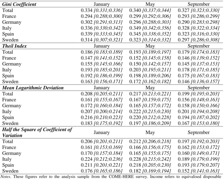
This Appendix describes the time series for the inequality indices (Tables A1 and A2). Table A1 shows that all relative-inequality measures, except in Germany, rose between January and May (and significantly so at the 10% level at least in the whole analysis sample and in Italy). However, relative inequality was lower in September than it was in January in every country, with these differences being significant at the 10% level everywhere except in France. The difference between the Gini indices in Spain in January and September is statistically significant at the 5% level. This is unsurprising: Spain is the only country where the cumulative shares of income were significantly higher at conventional levels for 8 out the 10 deciles of the income distribution between January and September (results available upon request). We find similar hump-shaped profiles in the other measures of relative inequality. As for the Gini index, the General Entropy measures are significantly lower in September than in January in every country bar France.

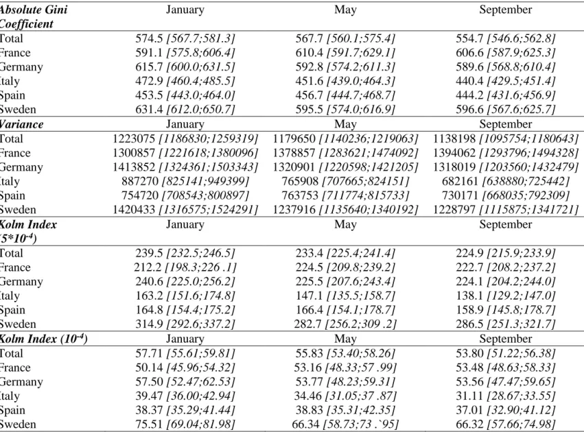
We then turn to absolute inequality in Table A2. Between January and May 2020, absolute inequality rose only in France and, to a lesser extent, Spain. By September 2020, absolute inequality was below its January value everywhere (significantly so for the whole sample and Italy) bar in France.

Figures A1 to A8 depict the evolution of all the afore-mentioned indices between January and September 2020 when we take into account the issues of attrition, national representativeness, grouped-data and unobserved income changes within income bands. They reveal that none of these issues seems to affect our conclusions about the evolution of relative and absolute inequality over the course of 2020.

(33)

30

Table A1: Relative Income Inequality Indices in COME-HERE over 2020

Gini Coefficient January May September

Total 0.334 [0.331;0.336] 0.340 [0.337;0.344] 0.327 [0.323;0.330] France 0.294 [0.288;0.300] 0.299 [0.292;0.306] 0.293 [0.286;0.299] Germany 0.302 [0.291;0.313] 0.296 [0.288;0.303] 0.290 [0.283;0.298] Italy 0.336 [0.330;0.342] 0.349 [0.342;0.356] 0.328 [0.322;0.334] Spain 0.339 [0.333;0.345] 0.345 [0.338;0.352] 0.323 [0.316;0.330] Sweden 0.314 [0.307;0.321] 0.323 [0.314;0.332] 0.297 [0.286;0.308]

Theil Index January May September

Mean Logarithmic Deviation January May September

Half the Square of Coefficient of

Variation January May September

Total 0.206 [0.201;0.211] 0.212 [0.206;0.218] 0.197 [0.192;0.203] France 0.161 [0.153;0.169] 0.166 [0.156;0.175] 0.162 [0.153;0.172] Germany 0.170 [0.157;0.184] 0.165 [0.155;0.175] 0.160 [0.149;0.171] Italy 0.224 [0.212;0.236] 0.228 [0.215;0.242] 0.189 [0.179;0.199] Spain 0.211 [0.201;0.221] 0.218 [0.205;0.230] 0.193 [0.179;0.207] Sweden 0.176 [0.165;0.186] 0.182 [0.169;0.194] 0.152 [0.141;0.163] Notes. These figures refer to the analysis sample from the COME-HERE survey. Income refers to equivalised disposable

(34)

31

Table A2: Absolute Income Inequality Indices in COME-HERE over 2020

Absolute Gini Coefficient

January May September

Variance January May September

Total 1223075 [1186830;1259319] 1179650 [1140236;1219063] 1138198 [1095754;1180643] France 1300857 [1221618;1380096] 1378857 [1283621;1474092] 1394062 [1293796;1494328] Germany 1413852 [1324361;1503343] 1320901 [1220598;1421205] 1318019 [1203560;1432479] Italy 887270 [825141;949399] 765908 [707665;824151] 682161 [638880;725442] Spain 754720 [708543;800897] 763753 [711774;815733] 730171 [668035;792309] Sweden 1420433 [1316575;1524291] 1237916 [1135640;1340192] 1228797 [1115875;1341721] Kolm Index (5*10-4₎

January May September

Total 239.5 [232.5;246.5] 233.4 [225.4;241.4] 224.9 [215.9;233.9] France 212.2 [198.3;226 .1] 224.5 [209.8;239.2] 222.7 [208.2;237.2] Germany 240.6 [225.0;256.2] 225.5 [207.6;243.4] 224.1 [204.2;244.0] Italy 163.2 [151.6;174.8] 147.1 [135.5;158.7] 138.1 [129.2;147.0] Spain 164.8 [154.4;175.2] 166.4 [154.1;178.7] 158.9 [145.8;178.7] Sweden 314.9 [292.6;337.2] 282.7 [256.2;309 .2] 286.5 [251.3;321.7]

Kolm Index (10-4₎ _January _May _September

Total 57.71 [55.61;59.81] 55.83 [53.40;58.26] 53.80 [51.22;56.38] France 50.14 [45.96;54.32] 53.16 [48.33;57 .99] 53.48 [48.63;58.33] Germany 57.50 [52.47;62.53] 53.77 [48.23;59.31] 53.56 [47.47;59.65] Italy 39.47 [36.00;42.94] 34.46 [31.05;37 .87] 31.11 [28.67;33.55] Spain 38.37 [35.29;41.44] 38.83 [35.31;42.35] 37.01 [32.90;41.12] Sweden 75.51 [69.04;81.98] 66.34 [58.73;73 .`95] 66.32 [57.66;74.98] Notes. These figures refer to the analysis sample from the COME-HERE survey. “Income” refers to equivalised

(35)

32

Figure A1: The evolution of Relative Income Inequality in COME-HERE over 2020 – Balanced Panel

(36)

33

Figure A2: The evolution of Absolute Income Inequality in COME-HERE over 2020 Balanced Panel

(37)

34

Figure A3: The evolution of Relative Income Inequality in COME-HERE over 2020 using Sample Weights

(38)

35

Figure A4: The evolution of Absolute Income Inequality in COME-HERE over 2020 using Sample Weights

(39)

36

Figure A5: The evolution of Relative Income Inequality in COME-HERE over 2020

(40)

37

Figure A6: The evolution of Absolute Income Inequality in COME-HERE over 2020

(41)

38

Figure A7: The evolution of Relative Income Inequality in COME-HERE over 2020 – Considering income changes

(42)

39

Figure A8: The evolution of Absolute Income Inequality in COME-HERE over 2020 – Considering income changes