A method to couple HEM and HRM two-phase flow models

HAL Id: hal-01265379

https://hal.archives-ouvertes.fr/hal-01265379

Submitted on 1 Feb 2016

HAL is a multi-disciplinary open access

archive for the deposit and dissemination of

sci-entific research documents, whether they are

pub-lished or not. The documents may come from

L’archive ouverte pluridisciplinaire HAL, est

destinée au dépôt et à la diffusion de documents

scientifiques de niveau recherche, publiés ou non,

émanant des établissements d’enseignement et de

A method to couple HEM and HRM two-phase flow

models

Annalisa Ambroso, Jean-Marc Hérard, Olivier Hurisse

To cite this version:

Annalisa Ambroso, Jean-Marc Hérard, Olivier Hurisse. A method to couple HEM and HRM two-phase

flow models. Computers and Fluids, Elsevier, 2009, 38, pp.738-756. �10.1016/j.compfluid.2008.04.016�.

�hal-01265379�

A METHOD TO COUPLE

HEM AND HRM TWO-PHASE FLOW MODELS

Annalisa Ambroso

, Jean-Marc H´

erard

, Olivier Hurisse

1_{Electricit´e de France, Division Recherche et D´eveloppement,´}

D´epartement M´ecanique des Fluides, Energies et Environnement, 6 quai Watier, 78401 Chatou cedex, FRANCE

jean-marc.herard@edf.fr, olivier.hurisse@edf.fr

2 _{Universit´e de Provence, Centre de Math´ematiques et d’Informatique,}

Laboratoire d’Analyse, Topologie et Probabilit´es - UMR CNRS 6632, 39 rue Joliot Curie, 13453 Marseille cedex 13, FRANCE

3 _{Commissariat `a l’Energie Atomique,}

Centre de Saclay, DEN-DM2S-SFME-LETR , F-91191 Gif-sur-Yvette, France,

annalisa.ambroso@cea.fr

We present a method for the unsteady coupling of two distinct two-phase flow models (namely the Homogeneous Relaxation Model, and the Homogeneous Equilibrium Model) through a thin interface. The basic approach relies on recent works devoted to the inter-facial coupling of CFD models, and thus requires to introduce an interface model. Many numerical test cases enable to investigate the stability of the coupling method.

I.

Introduction

We focus in this paper on the unsteady interfacial coupling of two distinct two-phase flow models that are commonly used in order to simulate water-vapour flows in nuclear power plants. We emphasize that we only deal with a steady coupling interface that separates the two codes. The main objective here is to prescribe meaningful boundary conditions on each side of this coupling interface for both codes associated with HEM and HRM models.

The Homogeneous Relaxation Model (denoted by the acronym HRM) is a four-equation model that is widely used in two-phase flow simulations. Most industrial codes within the nuclear community - for instance THYC (EDF) or FLICA (CEA) - rely on this model. This model requires computing approximations of solutions of two mass balance equations, a total momentum equation and a governing equation for the total energy balance of the mixture. Excluding source terms, this model is under conservative form. The only non-zero source contribution is on the right hand side of the governing equation of the liquid mass fraction.

∗_{Corresponding author} †_{PhD student}

This source tends to relax the current liquid mass fraction to the equilibrium mass fraction, which only depends on the mean pressure and the mean density. The underlying time scale is highly variable, and in practice it makes the source term very stiff, which may render the computation of the HRM model rather uneasy. Actually, the Homogeneous Equilibrium Model (acronym HEM) precisely stands for the counterpart of the HRM model when an equilibrium is achieved. It is thus a pure convective set of partial differential equations which govern the motion of the total mass, the global momentum and the total energy of the whole mixture. Both the HEM and the HRM models require defining appropriate equations of state (referred to as the EOS in the following) in order to account for both the ”pure vapour” phase, the ”pure liquid” phase but also the ”mixture” phase. These EOS are usually tabulated (see22, 30, 31_{), but we will focus here on simplified}

analytical EOS. This is essentially motivated by the fact that we do not wish to mix numerical drawbacks due to the use of realistic EOS and those connected with the formulation of the coupling techniques. In other words, we want to be ”optimal” in some sense in terms of EOS in order to concentrate on the main drawbacks of the coupling techniques.

In order to introduce the problem of the interfacial coupling of two existing codes, we need to define governing equations:

∂t(W ) + ∂n(Fn,L(W )) = 0 (1)

for the left code (xn= x · n < 0, t > 0), respectively, for the right code (xn> 0, t > 0):

∂t(W ) + ∂n(Fn,R(W )) = 0, (2)

where n is the unit normal to the plane and steady coupling interface, which is located at xn= 0. Moreover,

we assume that the two systems on each side are hyperbolic and invariant under frame rotation.

Quite recently, some authors have proposed two approaches in order to tackle the unsteady interfacial coupling of CFD models. Roughly speaking, the first approach favours the continuity of the conservative variable W , by enforcing W (xn = 0−, t) = W (xn = 0+, t) in a weak sense (see18, 20). This method has

been recently extended to the case of a generic variable Z(W ) (see2, 4_{and also}3, 10, 13_{). The second one relies}

on the basic paper by Greenberg and Leroux.21 _{It consists in introducing a colour function Y (x, t) where}

Y (x, t) = 1, if xn = x · n < 0, and Y (x, t) = 0 if xn= x · n > 0. Since the interface is steady, the function

Y verifies ∂t(Y ) = 0. Defining Fn(W ) = Y Fn,L(W ) + (1 − Y )Fn,R(W ), the fluxes at the steady coupling

interface can be computed by solving the Riemann problem associated with:

∂t(W ) + ∂n(Fn(W )) = 0, (3)

This method, which introduces the ”father model” (3) obviously privileges the conservation law. It has been used in.23, 26

More recently, a third approach has been proposed (2, 4_{). It combines the second method with the}

relax-ation methods.5, 6, 11 _{The coupling technique that is used herein makes use of the latter approach. Actually,}

we want here to take advantage of the fact that the HRM model may be viewed as the ”father model” of the HEM model. Another advantage of the third approach is that one may get rid of possible resonance phenomena, as underlined in2, 4_{for instance. This phenomena may arise when using the second approach if}

a genuinely non linear field overlaps the steady linearly degenerate field associated with the colour function Y . Though it is not clear whether this has drastic consequences, it seems indeed much more reasonable to avoid this problem that is not clearly understood (17_{) .}

The paper is organized as follows:

• Sections II and III are devoted to the presentation of both HEM and HRM models, but also on some of their properties (hyperbolicity, entropy inequality, positivity results for sufficiently smooth solutions). • We then present the coupling method in section IV. Special attention will be paid to the numerical

treatment of the coupling interface, which relies on: (i) an evolution step,

(ii) an instantaneous relaxation step,

This section also includes a brief description of the Finite Volume methods that will be applied in order to compute approximations of solutions in non coupled codes.

• Numerical results are displayed in section V. This includes basic test cases involving contact waves, shock waves and rarefaction waves, but also a schematic representation of the flow in a part of the primary coolant circuit in a nuclear power plant.

Throughout the paper, we will use the following notations: ρ stands for the density of the mixture, τ = 1/ρ is its specific volume and U represents the mean velocity of the mixture. Moreover P , C, e, h = e + P/ρ, E = e + U2_{/2 respectively stand for the pressure, the liquid mass fraction, the internal energy,}

the enthalpy, and the total volumetric energy of the mixture. The subscripts v and l respectively refer to the vapor and the liquid phases. The over-script s denotes saturated quantities.

II.

The Homogeneous Relaxation Model

This four-equation model can be derived from the six-equation two-fluid model. In the following we focus on specific closure laws and we detail some properties connected with these choices.

A. Closure laws

We consider that the two fluids have the same mean velocity, that is Ul− Uv = Ur = 0. In order to take

into account the mass transfer between the two phases, a source term ρΓ stands on the right hand side in the equation of the mass balance of the liquid phase. Thus the governing equations are:

         ∂t(ρC) + ∂x(ρCU ) = ρΓ ∂t(ρ) + ∂x(ρU ) = 0 ∂t(ρU ) + ∂x ¡ ρU2+ P¢= 0 ∂t(ρEHRM) + ∂x(U (ρEHRM+ P )) = 0 (4) with: EHRM def = eHRM(P, ρ, C) + U2 2 and eHRM(P, ρ, C) def = hHRM(P, ρ, C) − P ρ (5)

where the function hHRM(P, ρ, C) is the specific enthalpy that must be prescribed by the user. In practice

here, we will use the definition (10).

The set of physical relevant states for the system (4) is: ΩHRM

def

= {(ρ, U, P, C) / ρ ≥ 0, C ∈ [0, 1], P ≥ 0} (6) In order to close the system, we need to define hHRM and Γ.

• First, we write the enthalpy function hHRM. We choose the thermodynamic closures inspired by the

THYC and FLICA codes.22, 31 _{They consider the medium as the mixing of two fluids: liquid water}

and vapour. Moreover, the vapour is assumed to be in a saturation state, this implies that each thermodynamic function relative to this fluid only depends on one variable, say the pressure P . The two pure fluids are assumed to obey a usual γ closure law.

We note γv > 1 (respectively γl > 1) the adiabatic constant for the vapour (respectively the liquid),

and ev, hv, ρv and τvthe internal specific energy, specific enthalpy, density and specific volume for the

vapour (respectively el, hl, ρland τl the internal specific energy, specific enthalpy, density and specific

volume for the liquid).

We recall the following definitions: ep(ρ, P ) def = P (γp− 1)ρ and hp(ρ, P ) def = δpP τ with δp def = γp/(γp− 1) (7) for p = l, v.

We will use standard values in order to account for liquid and gas respectively : γl = 1.001 and

γv = 1.4. Moreover, we assume that if the pressure P stays in [PM IN, PM AX] the saturation curves

for the enthalpy and the volumetric fraction can be approached by the following functions: – Saturated Vapor: hsv(P ) def = AvP + Bv and τvs(P ) def = h s v(P ) δvP (8) – Saturated Liquid hsl(P ) def = AlP + Bl and τls(P ) def = h s l(P ) δlP (9)

Physically relevant saturation curves ensure that: τs

v(P ) > τls(P ) and hsv(P ) > hsl(P ). Typical values

of the coefficients PM IN, PM AX, Av < 0, Al, Bv and Blrelated to nuclear cooling conditions can be

found at the beginning of Section V.

We can now define the total specific enthalpy of the mixture: hHRM(P, ρ, C) def = Chl(P, ρl) + (1 − C)hsv(P ), (10) where ρl= ρC 1 1 − ρ(1 − C)τs v(P ) = C τ − (1 − C)τs v(P ) , (11)

This relation (11) is obtained by introducing the two void fractions αland αvfor the liquid and vapour

respectively, that are in agreement with αl+ αv= 1. Using the standard definitions of the partial mass

for the liquid and the mean density of the mixture:

αlρl= ρC and: ρ = αlρl+ αvρv

one may eliminate αl,v and inject ρv = ρsv(P ), in order to obtain ρl in terms of P, ρ, C, that is the

above relation (11).

In the following, the HRM model will refer to the set of equations (4), (5), (10). The enthalpy (10) of the model can be simplified, by using (7), (8).

ρhHRM(P, ρ, C) = δlP + ρ(1 − C)hsv(P )(1 −

δl

δv

) (12)

This simplified form of EOS will enable us to derive some technical results. Remark 1:

With this thermodynamic closure, the domain of validity of the HRM model is: DHRM

def

= {C ∈ [0, 1], P ∈ [PM IN, PM AX], (1 − C)τvs(P ) ≤ τ ≤ τvs(P )} (13)

where we have used (6), (11) and the constraint τl ∈]0, τvs(P )] to obtain the relation on the bounds of

τ .

• The source term Γ in the set of equations (4) allows the exchange of mass between the two phases. It depends on the density ρ, the pressure P and the liquid mass fraction C. Its form arises from the literature (see22, 31_): Γ = C(1 − C) τ0 ρτvs(P ) hs l(P ) − hl(P, ρl) hs v(P ) − hsl(P ) (14) where τ0 is a time scale.

For regular solutions, system ((4), (5)) can be written:          ∂t(C) + U ∂x(C) = Γ ∂t(ρ) + U ∂x(ρ) + ρ∂x(U ) = 0 ∂t(U ) + U ∂x(U ) +1_ρ∂x(P ) = 0 ∂t(P ) + U ∂x(P ) + ˆγHRMP ∂x(U ) = −Γ_∂∂CP(e(eH RMH RM)). (15) with: ˆ γHRM def = (P ∂P(eHRM))−1 µ P ρ − ρ∂ρ(eHRM) ¶ We will use this form to highlight some of its properties.

B. Hyperbolicity of the HRM model

In order to study the hyperbolicity of the HRM model, we focus on the convective part of (15) complemented with (5). Then the non-conservative equations on ρ, U , P and C are:

∂t      C ρ U P     +      U 0 0 0 0 U ρ 0 0 0 U τ 0 0 ˆγHRMP U     ∂x      C ρ U P     =      0 0 0 0      (16)

The following result is classic: Property 1

The system (16) is hyperbolic if and only if ˆγHRMP > 0. Its eigenvalues and right eigenvectors are recalled

below:

λ1= U − aHRM; r>1 = (0, ρ, −aHRM, ρa2HRM)

λ2= U ; r>2 = (1, 0, 0, 0)

λ3= U ; r>3 = (0, 1, 0, 0)

λ4= U + aHRM; r>4 = (0, ρ, +aHRM, ρa2HRM)

where we define the sound velocity aHRM by:

aHRM def = (ˆγHRMP/ρ)1/2 (17) Property 2 If we assume that : 1 < γl< γv and Av< 0

the system (16) is hyperbolic for all P ∈ [PM IN, PM AX], ρ > 0, C ∈ [0, 1].

We insist that this is not a necessary condition. Proof

Using the definition (12) of hHRM together with the relation ρeHRM = ρhHRM− P we obtain:

µ P ρ − ρ∂ρ(eHRM) ¶ = δlP ρ ∂P(eHRM) = τ (δl− 1) + (1 − C)(1 − δl δv) d dPh s v(P ) The term δlP

ρ is always positive, and a sufficient condition for ∂P(eHRM) to be positive is:

(1 −_δδl v ) d dPh s v(P ) > 0 Thanks to (8), we have: _dPd hs

v(P ) = Av, and Av is negative. Obviously, 1 < γl< γv implies: δv< δl. Thus,

ˆ

γHRMP is positive, which concludes the proof.

We remark that the numerical values in section V, equation (42), are such that Av < 0, and that γl,v

fulfill the condition above.

C. Some positivity results for the HRM model Remark 2:

We have introduced the source term Γ in (14). We can rewrite it in a form which will appear to be more convenient. We set : G2(P, ρ) def = ρτvsδlPτ s v(P ) − τls(P ) hs v(P ) − hsl(P ) and C¯def= τ s v(P ) − τ τs v(P ) − τls(P ) (18)

Since the saturation functions ensure that both τs

v(P ) > τls(P ) and hsv(P ) > hsl(P ), we know that G2> 0 if

P ∈ [PM IN, PM AX], and if ρ > 0. The source term may thus be rewritten:

Γ = (1 − C)¡ ¯C − C¢ G2(P, ρ) τ0

(19) The ODE

∂t(C) = Γ(P, ρ, C)

has two poles. The pole C = 1 is repulsive and the pole C = ¯C is attractive. The expression of the second pole will make sense for the HEM model. This remark will be used for numerical purposes (see system (39) and associated Appendix 2).

Positivity results:

We now want to highlight some properties of positivity of the regular solutions of ((4)-(5), (10), (14)), or alternatively (15), (14). The demonstration of the following results can be found in Appendix 4 (section A).

If we assume that U ∈ L∞_{(Ω × [0, T ]) and ∂}

x(U ) ∈ L∞(Ω × [0, T ]) then,

ρ ≥ 0

Moreover if we assume that ρ ∈ L∞_{(Ω × [0, T ]) and that P remains in [P}

M IN, PM AX],

C ≤ 1 and if the additional condition ¯C ≥ 0 is fulfilled then:

C ≥ 0

Nonetheless nothing ensures that ¯C remains in [0, 1], nothing ensures that P remains in [PM IN, PM AX], and

nothing ensures that ρl will remain positive.

Remark 3:

An analytical solution of the HRM model can go out of the domain DHRM (13). It is thus possible for a

”consistent and stable numerical approximation” to go out of DHRM. In practice, if a numerical solution

does not remain in this domain the computations will be stopped. D. Entropy and source terms

In this section we wonder whether the source term Γ may contribute to the entropy dissipation. We consider the functions SHRM : (P, ρ, C) 7→ SHRM(P, ρ, C) that are in agreement with:

a2HRM∂P(SHRM) + ∂ρ(SHRM) = 0 (20)

We introduce the entropy-entropy flux pair: (ηHRM, FηHRM)

ηHRM = −ρ ln(SHRM)

FηHRM = U ηHRM

Using a classical approach - that is: introducing a viscous contribution in governing equations, deriving the evolution equation of the entropy in that framework, and then passing to the limit by enforcing a vanishing viscosity (see19 _{for instance )- we know that smooth solutions of (4) agree with the entropy inequality:}

∂t(ηHRM) + ∂x

¡ FηHRM

¢

≤ 0 (21)

We now focus on the smooth solutions of the HRM model with the zero-order source term (4). These are such that (see Appendix 4, section B):

∂t(ηHRM) + ∂x¡FηHRM ¢ = Γη with: Γη= Γ ρ SHRM ∂P(SHRM) · ∂C(SHRM) ∂P(SHRM)− ∂C(eHRM) ∂P(eHRM) ¸

Thus, in order to comply with the entropy inequality (21), the source term Γ should agree with the relation: Γη ≤ 0

In order to specify conditions on Γ, we introduce the physical entropy: SHRM = P f (ρ, C)

with:

f (ρ, C) = f0(C)((1 + ρAv(1 − δl/δv)(1 − C)/(δl− 1))/ρ)γl

where the positive function f0(C) should fulfill: f0(1) = 1. Hence the above condition turns out to be :

Γ · ∂C(SHRM) ∂P(SHRM)− ∂C(eHRM) ∂P(eHRM) ¸ < 0

Using the expression of SHRM = P f (ρ, C) above, one can check that the form of the source term Γ does

not necessarily satisfy the constraint. This may be easily explained: the source term Γ has been picked up from the standard two-phase flow literature, whatever the EOS of the mean fluid is, which may result in a potential conflict. In practice, if one retains f0(C) = 1, the agreement will occur if and only if the source

III.

The Homogeneous Equilibrium Model

A. Governing equations

The Homogeneous Equilibrium Model is governed by a set of three equations in order to account for total mass, total momentum and total energy balances. These read:

     ∂t(ρ) + ∂x(ρU ) = 0 ∂t(ρU ) + ∂x ¡ ρU2_{+ P}¢_{= 0}

∂t(ρEHEM) + ∂x(U (ρEHEM+ P )) = 0

(22) with: EHEM def = eHEM(P, ρ) +U 2 2 and eHEM(P, ρ) def = hHEM(P, ρ) −P ρ (23)

where, again, the function hHEM(P, ρ) is the specific enthalpy, and must be prescribed by the user.

We want to ensure the compatibility of this thermodynamic closure with the HRM one, in a sense to be precised later. For this reason, we can restrain the domain of validity of system (22) to:

DHEM =

©

(ρ, P )/P ∈ [PM IN, PM AX], ρ > (τvs(P ))−1

ª

(24) Moreover, the thermodynamic relations for the liquid and the vapour (7), (8), (9) still hold.

First we set: Ceq(P, ρ) def = τ s v(P ) − τ τs v(P ) − τls(P ) (25) We also need to introduce two subdomains:

• the pure liquid domain Dl= {τ < τls(P ), P ∈ [PM IN, PM AX]}

• the two-phase region D2φ= {τls(P ) ≤ τ ≤ τvs(P ), P ∈ [PM IN, PM AX]}.

In order to complete (22), (23), we define the specific enthalpy hHEM(P, ρ) on the pure liquid domain

and on the two-phase domain:

• Pure liquid domain Dl: if Ceq > 1 or equivalently τ < τls(P ) :

hHEM(P, ρ) def

= hl(P, ρ)

• Two-phase domain D2φ : if 0 ≤ Ceq≤ 1 or equivalently τls(P ) ≤ τ ≤ τvs(P ) :

hHEM(P, ρ) def

= Ceqhl(P, ρl(P, ρ, Ceq)) + (1 − Ceq)hsv(P )

Using (11) and (25), we get: ρl(P, ρ, C = Ceq) = 1/τls(P ). Hence the enthalpy of the HEM model in the

two-phase domain D2φ, simply reads :

hHEM(P, ρ) = Ceqhsl(P ) + (1 − Ceq)hsv(P ) (26)

The enthalpy hHEM is continuous at the boundary between the two domains D2φ and Dl (i.e. continuous

at Ceq= 1). Nevertheless, its derivatives are not continuous.

In the following, the HEM model will refer to the set of equation (22), (23) with the above definitions (26) of hHEM and the saturation curves.

Remark 4:

It is important to note that Ceq(P, ρ) = ¯C. The relaxation source term (19) of the HRM model can now be

written:

Γ = (1 − C) (Ceq(P, ρ) − C)

G2(P, ρ)

τ0

Then C = Ceq(P, ρ) is a curve for the equilibrium Γ = 0.

Remark 5:

There is a compatibility of the EOS of the HEM model with the EOS of the HRM model. The relation ρl(P, ρ, C = Ceq) = 1

τs l(P )

implies that:

hHEM(P, ρ) = hHRM(P, ρ, C = Ceq)

In section IV, we study the coupling of these HEM and HRM models. The previous choice on compatible EOS will allow us to focus on the main differences between models rather than on discrepancies linked with inhomogeneities of EOS. The latter problem is addressed in.4, 10

B. Hyperbolicity

In order to study the hyperbolicity of the HEM model, we focus on (22). Then the non-conservative equations on ρ, U and P are: ∂t    ρ U P    +    U ρ 0 0 U τ 0 γˆHEMP U    ∂x    ρ U P    =    0 0 0    (28) with: ˆ γHEM = (P ∂P(eHEM))−1 µ P ρ − ρ∂ρ(eHEM) ¶ Property 3

The system (28) is hyperbolic if and only if ˆγHEMP > 0. Its eigenvalues and right eigenvectors are recalled

below:

λ1= U − aHEM; r>1 = (ρ, −aHEM, ρa2HEM)

λ2= U ; r>2 = (1, 0, 0)

λ3= U + aHEM; r>3 = (ρ, +aHEM, ρa2HEM)

where the sound velocity aHEM is defined by:

aHEM def

= (ˆγHEMP/ρ)1/2 (29)

Since the derivatives of eHEM are not defined in the whole domain DHEM, ˆγHEM is only defined inside

the subdomains Dl and D2Φ.

Property 4

The HEM model is hyperbolic inside the pure liquid domain and inside the two-phase domain. Proof

The sound speed reads:

• In the pure liquid domain: aHEM =√γlP τ =

q

δl

δl−1P τ ∀(τ, P ) ∈

◦

Dl

• In the two-phase domain the formulas are cumbersome and no sufficient condition clearly appears to ensure the positivity of a2

HEM. For all couple (τ, P ) in ◦ D2Φ, we have: a2 HEM = ³ P ρ − ρ∂ρ(e) ´ ρ∂P(e) (30) with: _µ P ρ − ρ∂ρ(e) ¶ = ρ∂ρ(Ceq) (hsv− hsl)

∂P(e) = −τ + ∂P(Ceq) (hsl− hsv) + Ceq d dPh s l+ (1 − Ceq) d dPh s v

Nonetheless it can be shown that, with our choices for the saturation curves and for the chosen perfect gas coefficients, P

ρ − ρ∂ρ(e) and ∂P(e) remain positive inside the two-phase domain D2Φ.

C. Some positivity results for the HEM model

Again, if we consider smooth solutions of the HEM model (28), with positive initial conditions and -inlet-boundary conditions for ρ and P , we are ensured that the mean density will remain positive, and also that the mean pressure P will remain positive for (x, t) ∈ Ω × [0, T ] provided that U, ˆγHEM and ∂x(U ) lie in

L∞_{(Ω × [0, T ]) (for more details, see Appendix 4).}

However, nothing guarantees that for smooth solutions, ρ will agree with ρ > (τvs(P ))−1 and P will

IV.

A method to couple HEM and HRM models

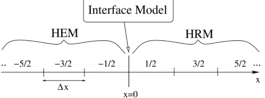
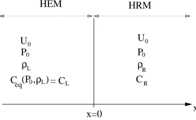
We want to couple an ”HEM” code and an ”HRM” code through an interface x = 0. The HEM domain will correspond to x < 0, and the HRM domain to x > 0 (see figure 1) .

One of the main difficulties which arise when one aims at coupling the HRM and HEM models is due to the fact that the liquid mass fraction C is governed by a PDE in the HRM, and issues from a local constraint C = Ceq(P, ρ) in the HEM model. We propose to couple both models using a ”father interface model”

with an instantaneous relaxation process at the interface. In26 _{, a similar approach was used to couple a}

one dimensional code and a two dimensional code, following ideas from21 _{. In the present approach, we}

rather choose to proceed as in2, 4 _{. The main advantage is that one can get rid of the possible resonance}

phenomenon, since the set of right eigenvectors of the model we propose spans the whole phase space. A. The interface model

We first rewrite the HEM set of equations. This is achieved introducing a PDE with a source term containing an instantaneous relaxation term:

∂t(ρC) + ∂x(ρU C) = µρ(Ceq(P, ρ) − C)

The set of equations for the HEM model (using the confusing notation E instead of EHEM on purpose) thus

writes (for x ∈ R− _{and t ∈ R}+_{) :}

         ∂t(ρC) + ∂x(ρU C) = µρ(Ceq(P, ρ) − C) ∂t(ρ) + ∂x(ρU ) = 0 ∂t(ρU ) + ∂x¡ρU2+ P¢= 0 ∂t(ρE) + ∂x(U (ρE + P )) = 0 (31)

with the parameter µ > 0. We also recall that the governing equations for (x, t) ∈ R+_{× R}+ _{are given by}

the HRM model (4), (5), (10).

We may now introduce the ”father model”. For that purpose we define a new variable Y (x, t) depending on time and space, which is usually called the ”color variable”. The ”father model” is governed by the following set of equations (for x ∈ R and t ∈ R+_):

             ∂t(ρC) + ∂x(ρCU ) = ρT ∂t(ρ) + ∂x(ρU ) = 0 ∂t(ρU ) + ∂x¡ρU2+ P¢= 0 ∂t(ρE) + ∂x(U (ρE + P )) = 0

∂t(ρY ) + ∂x(ρU Y ) = λ(Y0− Y )

(32) with: E = Y eHRM(P, ρ, C) + (1 − Y )eHEM(P, ρ) + u2 2 and T = Y Γ + (1 − Y )µ(Ceq− C)

At the time t = 0 we initialize Y (x, 0) = Y0(x) such that Y0(x) = 1 if x is in the HRM domain and Y0(x) = 0

if x is in the HEM domain. In the following the parameters λ and µ will formally be set to +∞ (instanta-neous relaxation).

We may define a sound speed a for this interface model, which reads: a2=a 2 HRMY ∂P(eHRM) + a2HEM(1 − Y )∂P(eHEM) Y ∂P(eHRM) + (1 − Y )∂P(eHEM) (33) Property 5

Proof

Starting from (32), and focusing on regular solutions, the convective part of the first three equations and the fifth equation may be rewritten as follows:

         ∂t(C) + U ∂x(C) = 0 ∂t(ρ) + U ∂x(ρ) + ρ∂x(U ) = 0 ∂t(U ) + U ∂x(U ) + τ ∂x(P ) = 0 ∂t(Y ) + U ∂x(Y ) = 0 (34)

Meanwhile, the total energy equation is equivalent to: (

(Y ∂P(eHRM) + (1 − Y )∂P(eHEM))(∂t(P ) + U ∂x(P ))

+(Y ∂ρ(eHRM) + (1 − Y )∂ρ(eHEM))(∂t(ρ) + U ∂x(ρ)) + (P/ρ)∂x(U ) = 0

(35) Thus, using definitions of aHRM and aHEM from (17) and (29), the definition of a given by (33) and applying

(34) enables to derive the governing equation for the mean pressure as: ∂t(P ) + U ∂x(P ) + ρa2∂x(U ) = 0

We know from the study of the HEM and HRM models that ∂P(eHRM), a2HRM are positive if (C, ρ, P ) is in

the domain DHRM, and that ∂P(eHEM), and a2HEM are positive if (ρ, P ) lie in DHEM. Furthermore, the

system (32) ensures that if Y0is in [0, 1], Y remains in [0, 1]. Hence a2is positive. Therefore, a straightforward

and classic calculation enables to exhibit eigenvalues:

λ1,2,3= U, λ4= U − a, λ5= U + a

One may easily check that the associated right eigenvectors span R5_{. We may then conclude that the}

convective part of system (32) is hyperbolic if (C, ρ, P ) ∈ DHRM and (ρ, P ) ∈ DHEM.

B. Numerical scheme

All methods described herein rely on the Finite Volume method (12, 19_{) . We restrict here to the so-called}

”first-order” schemes. As an approximate Godunov scheme, we will apply VFRoe-ncv using the non con-servative variable (ρ, U, P ) for the HEM system and (ρ, U, P, C) for the HRM system (see7, 15 _{for details on}

these approximate Godunov schemes). The coupling interface model which has been introduced above will be used to compute ”fluxes” at the interface between the two domains.

HEM

HRM

Interface Model

...

...

Figure 1. Notations and models.

Let us introduce a fixed uniform mesh space ∆x and a time step ∆t in agreement with a CFL condition. We set for all integers j and n ,

xj+1/2= (j +

1

2)∆x, xj = j∆x, t

n_{= n∆t}

The cell j + 1/2 is delimited by the interface j located in xj and the interface j + 1 located in xj+1, and its

the variable W at the time tn _{in the cell j + 1/2. The HEM domain (and the HRM domain respectively) is}

composed of all the cells j + 1/2 < 0 (respectively of all the cells j + 1/2 > 0, see figure 1). The conservative variables will be denoted by WHEM = (ρ, ρU, ρEHEM)>in the HEM domain, WHRM = (ρC, ρ, ρU, ρEHRM)>

in the HRM domain and by WIN T = (ρC, ρ, ρU, ρE, ρY )> for the interface model.

We assume that Y_j+1/2n = 0 for all j + 1/2 < 0 and Y_j+1/2n = 1 for all j + 1/2 > 0 at a discrete time tn_{. The numerical scheme which is used to compute the variable at time step t}n+1_{= t}n_{+ ∆t contains three}

steps:

1) A convection step, tn_{→ t}n˜_.

2) An instantaneous relaxation on Y , tn˜ _{→ t}nˆ_.

3) A finite relaxation step, tˆn_{→ t}n+1_.

1. The convection step, tn_{→ t}˜n

This step of the scheme does not take into account the different source terms. The fluxes are computed at each interface j.

(i) For all interface j ≤ −1 (HEM domain) we apply the VFRoe-ncv scheme using the variable (ρ, U, P )>

on the convective part of the system (22). The flux is denoted Fn HEM,j.

(ii) For all interface j ≥ 1 (HRM domain) we apply VFRoe-ncv scheme using the variable (C, ρ, U, P )>_on

the convective part of the system (4). The flux is denoted Fn HRM,j.

(iii) At j = 0 (the coupling interface) the flux is built with a modified VFRoe-ncv scheme which uses the variable (C, ρ, U, P, Y )> _{in order to compute approximate interface states in the solution of the}

one-dimensional Riemann problem associated with the system (32). The left state in the initial condition of the Riemann problem is

((ρCeq(P, ρ))n−1/2, ρ n

−1/2, (ρU ) n

−1/2, (ρEHEM)n−1/2, (ρY ) n −1/2)

>

and the right state in the initial condition is

((ρC)n_1/2, ρn_1/2, (ρU )n_1/2, (ρEHRM)n1/2, (ρY ) n 1/2)

>

The flux is denoted Fn

IN T. Details on the computation of FIN Tn are given in Appendix 1.

Once the fluxes have been computed for all interfaces, the value of the cell is updated using the formula: • If j + 1/2 ≤ −3/2 WHEM,j+1/2n˜ − WHEM,j+1/2n + ∆t ∆x ¡ FHEM,jn − FHEM,j−1n ¢ = 0 • If j + 1/2 ≥ 3/2 WHRM,j+1/2n˜ − WHRM,j+1/2n + ∆t ∆x ¡ FHRM,jn − FHRM,j−1n ¢ = 0 • If j + 1/2 = −1/2 à WHEM ρY !n˜ −1/2 − à WHEM ρY !n −1/2 + ∆t ∆x à (F2−5)nIN T− à Fn HEM,−1 (ρU Y )n HEM,−1 !! = 0 The flux (F2−5)nIN T is composed of the second, third, fourth and fifth components of FIN Tn

• If j + 1/2 = 1/2 Ã WHRM ρY !n˜ 1/2 − Ã WHRM ρY !n 1/2 + ∆t ∆x ÃÃ Fn HRM,1 (ρU Y )nHRM,1 ! − FIN Tn ! = 0 An important point to underline is that: Y˜n

j+1/2 = Yj+1/2n in all the cells, except in the cell j = 1/2 if

Un

2. Instantaneous relaxation step, tn˜ _{→ t}nˆ

For this step we consider the ODE system on the whole domain (x ∈ R):              ∂t(ρC) = 0 ∂t(ρ) = 0 ∂t(ρU ) = 0 ∂t(ρE) = 0

∂t(ρY ) = λ(Y0− Y ) with λ = +∞

⇐⇒              ∂t(ρC) = 0 ∂t(ρ) = 0 ∂t(ρU ) = 0 ∂t(ρE) = 0 Y = Y0 (36)

This can be rewritten in terms of discrete variables (for all k) as:              (ρC)ˆn k = (ρC)nk˜ ρnkˆ = ρnk˜ (ρU )ˆn k = (ρU )nk˜ (ρE)nˆ k = (ρE)nk˜ Yˆn k = Yk0 and thus              Cnˆ k = Ck˜n ρˆnk = ρ˜nk Unˆ k = Ukn˜ enˆ k = enk˜ Ynˆ k = Yk0 (37)

This step is totally transparent with respect to physical conservative variables. Let us call k the cell j + 1/2 for which Yn˜

j+1/2 6= Yj+1/2n , for all the other cells we have Yj+1/2˜n = Yj+1/20 . The fourth equation of (37)

implies that the pressure changes in the cell k during the current step. Indeed equations (37) imply: e(Pknˆ, ρ˜nk, Ckn˜, Yknˆ) = e(Pkn˜, ρnk˜, Ckn˜, Ykn˜) (38)

Thus Ynˆ

k 6= Ykn˜ implies that Pknˆ6= Pk˜n.

3. The finite time relaxation step, tnˆ_{→ t}n+1

In this final step we compute the source term T . In the HEM domain (that is: x < 0), this simply corresponds to the following update:

Cn+1_{= C}

eq(Pnˆ, ρnˆ)

In the HRM domain (that is: x > 0), it urges to find approximations of          ∂t(ρC) = ρΓ ∂t(ρ) = 0 ∂t(ρU ) = 0 ∂t(ρE) = 0 (39)

In terms of the non-conservative variables (C, ρ, U, P ), and restricting to regular solutions, (39) is equivalent

to: _         ∂t(C) = Γ ∂t(ρ) = 0 ∂t(U ) = 0 ∂t(P ) = −(∂P(eHRM))−1∂C(eHRM) Γ (40)

The time scheme which is used to discretize (40) is detailed in Appendix 2. It provides Cn+1 _{and P}n+1_,

while we get ρn+1= ρˆn and Un+1= Uˆn. The final update of conservative variables is achieved through:                (ρC)n+1_{= ρ}nˆ_Cn+1 ρn+1_{= ρ}ˆn (ρU )n+1_{= (ρU )}nˆ (ρE)n+1_{= ρ}nˆ³_e HRM(Pn+1, ρˆn, Cn+1, Ynˆ) +(U ˆ n )2 2 ´ (ρY )n+1_{= (ρY )}nˆ (41)

C. Remark 6:

• The convection step (thanks to the VFRoe-ncv scheme and the respect of the CFL condition) and the instantaneous relaxation step maintain the discrete liquid mass fraction Cˆn _{in [0, 1]. Moreover, if}

the discrete values of the equilibrium liquid mass fraction Ceq remain in [0, 1] during the finite time

relaxation computation, Cn+1_{will remain in [0, 1] (see Appendix 2).}

• The introduction of the fictitious variable Y does not lead to any modification of the left and right codes. Actually, the convection step implicitly provides boundary conditions on both sides of the coupling interface.

V.

Numerical results

Many test cases involving single waves, and in particular contact waves enable us to check that numerical methods used within each code are well-suited. More precisely, the exact analytical form of the internal energy, for both the HEM and the HRM models, is such that the approximate Godunov scheme VFRoe-ncv (using variables U, P, ρ and U, P, ρ, C for HEM and HRM models respectively) perfectly preserves these pure contact waves on coarse and fine meshes (see14_{). This is still true for the coupled HEM/HRM model, for}

similar reasons (see Appendix 3).

The different parameters will be set as follows:

PM IN = 0.1 105P a and PM AX = 200 105P a

γl= 1.001 and γv= 1.4

The form of the saturation curves is obtained using the following numerical values: hs

l = AlP + Bl hsv= AvP + Bv

with the coefficients:

Al= 8.18 10−2 Bl= 1.91 105 Av= −8.32 10−3 Bv= 2.58 106 (42)

The whole data correspond to nuclear cooling conditions.

We successively consider two different test cases which correspond to:

• the computation of Riemann problems including shock waves, contact waves and rarefaction waves, • a schematic computation of the flow in the coolant circuit of a nuclear power plant.

A. Riemann problems

We consider in this section a computational domain : x ∈ [−1, 1] which is discretized using a uniform mesh. We will compare for different mesh sizes, the results obtained with:

• The Homogeneous Equilibrium Model over the whole computational domain, • The Homogeneous Relaxation Model over the whole computational domain,

• The coupling configuration in which HEM is used for x < 0, HRM is used for x > 0, and the coupling technique described in section IV is applied for x = 0.

Hence, we will be able to compare the results of the coupled case with those obtained with a ”reference solution”, which will correspond with either the HRM results (or the HEM results) computed on a very fine mesh. In the nuclear community, the most widely used reference is the HRM model.

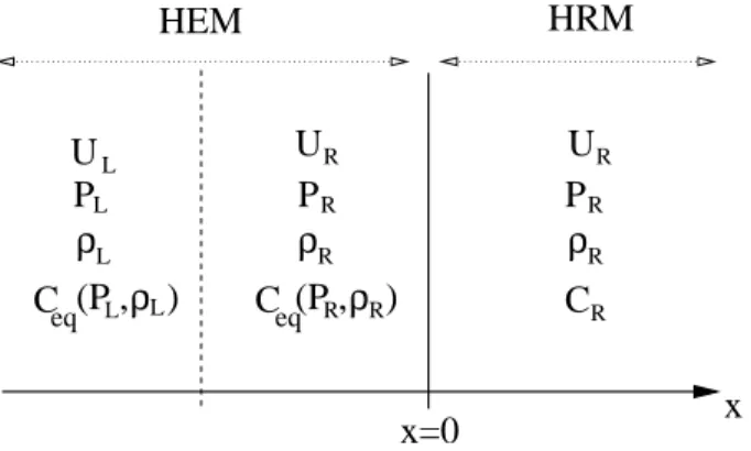
We focus here on test cases that are based on Riemann problems, where the initial discontinuity will be located either in the HEM code (x = −0.25), or in the HRM code ( x = +0.25), as described in figures 2 and 3. The main goal here is to observe the behavior of transmitted and reflected waves through the interface x = 0, and the numerical pollution due to the coupling scheme.

We emphasize that :

• Three different meshes will be used. An ”industrial” mesh with 100 cells (fifty cells within each code), a medium size mesh with 500 cells, and a fine mesh including 10000 cells that will provide ”almost converged” solutions.

• Rarefaction waves will be investigated, with special emphasis on the reflected and transmitted waves through the coupling interface. The counterpart including the propagation of shock waves through the coupling interface is reported in27_{. Rarefaction waves are of special interest in the nuclear framework,}

x

x=0

U

P

U

U

C

ρ

P

P

ρ

C (P , )

ρ

C (P , )

ρ

ρ

HEM

HRM

Figure 2. First configuration for initial data, the initial discontinuity is in the HEM domain

x

U

P

U

U

C

ρ

P

P

ρ

C (P , )

ρ

ρ

HEM

HRM

x=0

C

Figure 3. Second configuration for initial data, the initial discontinuity is in the HRM domain

• The time relaxation parameter τ0= 10−3 will be used. (similar tests with a different time scale τ0= 1

are reported in27_{) . In fact, when τ}

0 decreases, the similarity in the behaviour of the HRM and the

HEM models improves.

In each case, two series of results are shown:

• We have gathered computations for the HEM model, HRM model and the HEM/HRM simulation on coarse meshes in order to highlight the influence of the coupling in industrial configuration (see figures 4 and 6).

• Fine mesh computations for the HEM model and HRM model have been performed. They are plotted together with the results of the HEM/HRM simulation for all the meshes on the figure 5 and 7. Hence, results include (see figures 4, 6):

• a computation of the HEM model on the whole domain, using a mesh with 100 cells (circles); • a computation of the HRM model on the whole domain, using a mesh with 100 cells (triangles); • a computation of the coupled case HEM (x < 0)-HRM (x > 0), using a mesh with 100 cells (plain

line). .

A comparison is also made between results for (see figures 5,7):

• the ”converged” HEM model on the whole domain, using a mesh with 10000 cells (circles); • the ”converged” HRM model on the whole domain, using a mesh with 10000 cells (triangles);

• the ”converged” coupled case HEM (x < 0)-HRM (x > 0), using a mesh with 10000 cells (plain line); • the coupled case HEM (x < 0)-HRM (x > 0), using coarse meshes with 100, 500 cells ( dotted line,

dashed line). .

In each case we plot numerical results before the contact discontinuity hits the coupling interface x = 0. The time step agrees with the classical CFL condition . The implicit treatment of source terms implies no additional constraint. Numerical experiments include:

• a rarefaction wave travelling from the HEM code to the HRM code; • a rarefaction wave travelling from the HRM code to the HEM code

The dual case of shock waves is investigated in27 _{, and the last industrial test case contains such a}

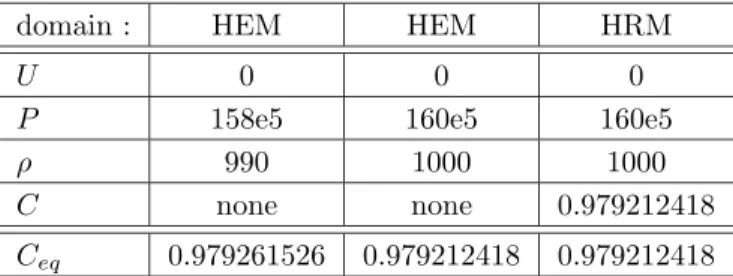
1. Test 1 : A rarefaction wave traveling from HEM domain to HRM domain Initial conditions are :

domain : HEM HEM HRM

U 0 0 0

P 158e5 160e5 160e5

ρ 990 1000 1000

C none none 0.979212418

Ceq 0.979261526 0.979212418 0.979212418

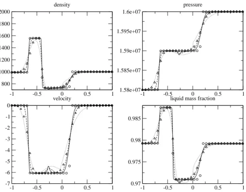
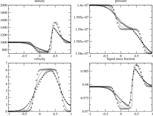
The initial discontinuity has been set at x = −0.25, that is inside the HEM domain. A rarefaction wave trav-els towards the right and goes through the coupling interface (x = 0), a shock wave travtrav-els to the left, and is followed by a left-going contact discontinuity. Results have been plotted at time t = 0.025. We notice that for the HEM computation, the whole right-going rarefaction wave has passed the coupling interface at that time. Associated results for the sole HRM model are indeed rather close to the solutions computed with the sole HEM model. Turning then to the coupled situation, we note that the rarefaction wave coming from the HEM code does not introduce too much pollution when passing through the coupling interface, though one can notice a sharp behaviour of the pressure field around x = 0, when the mesh is too coarse (100 cells, corresponding to the plain line on figure 4). In the coupled computation, the approximate solution in the HRM domain (respectively in the HEM domain) tends to stick immediately to the pure HRM solution (respectively to the pure HEM solution).

Another point seems worth being underlined. On the coarser mesh, one can notice (see figure 4 and 5 for instance) a sharp variation on velocity and density profiles which is located around the steady interface x = 0 . This pollution tends to decrease and clearly moves away from this interface when the mesh is refined.

-1 -0.5 0 0.5 1 800 1000 1200 1400 1600 1800 2000 density -1 -0.5 0 0.5 1 1.58e+07 1.585e+07 1.59e+07 1.595e+07 1.6e+07 pressure -1 -0.5 0 0.5 1 -7 -6 -5 -4 -3 -2 -1 0 velocity -1 -0.5 0 0.5 1 0.97 0.975 0.98 0.985

liquid mass fraction

Figure 4. Test 1. Constant time scale τ0 = 10−3_{. Circles=HEM 100 cells, triangles=HRM 100 cells,}

-1 -0.5 0 0.5 1 800 1000 1200 1400 1600 1800 2000 density -1 -0.5 0 0.5 1 1.58e+07 1.585e+07 1.59e+07 1.595e+07 1.6e+07 pressure -1 -0.5 0 0.5 1 -7 -6 -5 -4 -3 -2 -1 0 velocity -1 -0.5 0 0.5 1 0.97 0.975 0.98 0.985

liquid mass fraction

Figure 5. Test 1. Constant time scale τ0 = 10−3. Circles=HEM 10000 cells, triangles=HRM 10000 cells,

2. Test 2 : A rarefaction wave traveling from HRM domain to HEM domain Initial conditions are now the following:

domain : HEM HRM HRM

U 0 0 0

P 160e5 160e5 158e5

ρ 1000 1000 990

C none 0.979212418 0.979261526 Ceq 0.979212418 0.979212418 0.979261526

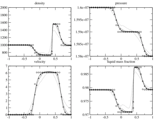
The initial discontinuity is now in the HRM domain, and is located at x = 0.25. A rarefaction wave travels to the left and goes through the coupling interface (x = 0). Meanwhile a shock wave travels to the right boundary, and is followed by a contact discontinuity that travels towards the right. Results are still plotted at time t = 0.025. At that time, the left-going rarefaction wave is entirely in the HEM domain in the sole HEM computation.

Remarks pertaining to the previous test case still hold. The mesh refinement helps much to improve the accuracy of the approximate solution in each subdomain. In the coupled simulation, the approximate solution is much more monotone around the coupling interface when the mesh is refined (see figure 7).

-1 -0.5 0 0.5 1 800 1000 1200 1400 1600 1800 2000 density -1 -0.5 0 0.5 1 1.58e+07 1.585e+07 1.59e+07 1.595e+07 1.6e+07 pressure -1 -0.5 0 0.5 1 0 1 2 3 4 5 6 7 velocity -1 -0.5 0 0.5 1 0.97 0.975 0.98 0.985

liquid mass fraction

Figure 6. Test 2. Constant time scale τ0 = 10−3_{. Circles=HEM 100 cells, triangles=HRM 100 cells,}

-1 -0.5 0 0.5 1 800 1000 1200 1400 1600 1800 2000 density -1 -0.5 0 0.5 1 1.58e+07 1.585e+07 1.59e+07 1.595e+07 1.6e+07 pressure -1 -0.5 0 0.5 1 0 1 2 3 4 5 6 7 velocity -1 -0.5 0 0.5 1 0.97 0.975 0.98 0.985

liquid mass fraction

Figure 7. Test 2. Constant time scale τ0 = 10−3. Circles=HEM 10000 cells, triangles=HRM 10000 cells,

B. Test 3 : A test case in a nuclear power plant

The next test case corresponds to the schematic one dimensional flow in a nuclear power plant. The length of the pipes is 80 m. It includes a part of the coolant circuit containing the core on the left side of the coupling interface (i.e. −40 < x < 0) where the governing set of equations is the HEM model. The core is located in the interval [−22, −18]. The total length of the core is the true core length (buoyancy effects can be neglected). The core section is equal to 3.5 m2_{. The HRM model is used on the right side of the coupling}

interface (i.e. 0 < x < 40). Before the beginning of the computation, the velocity, density and pressure profiles are uniform and equal to: U = 10 ms−1_{, ρ = 700 kgm}−3_{, P = 150 10}5_{P a ; moreover C = C}

eq(P, ρ)

in the HRM part of the coolant circuit. The fluid is not heated before the beginning of the computation, and the core is suddenly plugged in the coolant circuit at that time. Then the heat source Φ(x, t > 0) is equal to 0 outside the core. Within the core region (x ∈ [−22, −18]), and for t > 0, the uniform local heat source is Φ(x, t) = Φ0= 300.106/4. Thus, within the core region, the total heat power is 300 × 106W .

In this particular test case the constants Av, Bv, Al, and Blhave been estimated with PM IN = 140 105P a

and PM AX = 160 105P a using the Thetis software30. The uniform mesh contains 500 nodes. The governing

set of equations in the left part is the set of equations of the HEM model (22) with an equation for the total energy which takes the heat source into account:

∂t(ρE) + ∂x(U (ρE + P )) = Φ(x, t)

Results have been plotted at four distinct instants.

• At t = T1, the right-going shock wave, which is coming from the right side of the core, and which is

due to the sudden heating in the core region, has not hit the coupling interface yet (dashed line on figure 8).

• At t = T2, the same right-going shock wave has already moved through the coupling interface (plain line

on figure 8). One can easily observe at t = T2the reflected wave in the interval [−10, 0], either focusing

on the pressure profile, the density profile or the velocity profile. The amplitude of this reflected wave is small compared with the one of the associated shock wave.

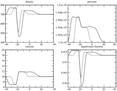
• At t = T3, the right-going contact wave has not passed the coupling interface yet (dashed line on figure

9). This contact wave is of course characterized by locally uniform pressure and velocity profiles. At that time, the right going shock wave has not reached the right exit. The behaviour of the coupling interface seems almost perfect, which is in agreement with test cases involving a contact wave travelling from the HEM domain towards the HRM domain (see27_{) .}

• At t = T4, the contact wave is on the right side of the coupling interface (x = 0) (plain line on figure

9). Once again, everything is correct around the coupling interface (x = 0). At that time t = T4, the

right-going shock wave has gone outside the computational domain. One can notice the influence of the right exit boundary which generates a reflected wave in the computational domain. This is due to the fact that crude ”Neumann-type” boundary conditions have been imposed in this test case.

-40 -20 0 20 40 400 500 600 700 800 density -40 -20 0 20 40 1.5e+07 1.502e+07 1.504e+07 1.506e+07 1.508e+07 1.51e+07 pressure -40 -20 0 20 40 6 8 10 12 14 16 18 20 velocity -40 -20 0 20 40 0.96 0.965 0.97 0.975

liquid mass fraction

Figure 8. Test 3. Interaction of the shock wave with the coupling interface. Dashed line (t = T1): the shock

wave has not hit the coupling interface. Plain line (t = T2) : the shock wave has passed the coupling interface.

-40 -20 0 20 40 400 500 600 700 800 density -40 -20 0 20 40 1.5e+07 1.502e+07 1.504e+07 1.506e+07 1.508e+07 1.51e+07 pressure -40 -20 0 20 40 6 8 10 12 14 16 18 20 velocity -40 -20 0 20 40 0.96 0.965 0.97 0.975

liquid mass fraction

Figure 9. Test 3. Interaction of the contact wave with the coupling interface. Dashed line (t = T3): the contact wave has not hit the coupling interface. Plain line (t = T4) : the contact wave has passed the coupling interface.

VI.

Conclusion

In this paper, we study the coupling of two different codes that provide numerical approximations of HEM and HRM models when applying industrial closure laws. It may be seen as a companion work of2 in which different coupling techniques are proposed - including the state coupling and the flux coupling approaches - and compared in an idealized thermodynamic frame. Here, we analyze one of these methods when the thermodynamic closures mimick the ones used in industrial codes. The two models HEM and HRM have been recalled, together with closure laws including EOS. We have chosen here a coupling method, that makes use of relaxation techniques. It is essentially different from the one that has been investigated in,26

which basically relies on ideas introduced by Greenberg and Le Roux (21_{) . Its simplicity is appealing, and}

it enables us to circumvent the tough problem of resonance at the coupling interface.

Some properties of both models, and the main properties of algorithms involved in associated codes have been given or recalled. Some properties of the coupling method have also been detailed. One may say that the whole approach is rather efficient, and we would like to emphasize the rather nice behaviour of the coupled approach when contact waves travel through the coupling interface. The reader must be aware that some numerical properties deeply rely on the approximate Godunov schemes (14_{) which are used in}

both codes. The coupling approach preserves the conservative form of mass, momentum and total energy equations. It also seems worth emphasizing the following features:

• If one restricts to coarse meshes, which is obviously the correct framework for industrial applications, it also occurs that incompatibilities between formulations may be smoothed with this formulation, owing to the dissipative nature of upwinding techniques which have been applied inside codes and at the coupling interface. This is indeed flagrant if one focuses on relaxation time scales. Some of the numerical results presented in27 _{confirm that one can cope with decorrelated signals (owing to very}

large relaxation times in the HRM model) on coarse meshes, but that this no longer holds when refining the mesh. This is much in favour of the present coupling approach, since it may be understood as a tool which automatically checks whether both models on each side of the interface are in agreement or not.

• A much deeper insight on thermodynamics is actually deserved. On the basis of4_{, we know that small}

discrepancies among EOS may result in rather high differences in results. Special emphasis should be given on the respective saturation curves for the liquid phase and the vapour phase. Some comments may be picked up in this manuscript, which might perhaps help improving the global formulation (see Appendix 4). The reader is also referred to.8, 28

• In this work, we have focused on compatible closure laws for the HEM and HRM models, and this results in a rather good behaviour in the coupling of both models. We recall that the case of the interfacial coupling of models involving different thermodynamics has been examined in4 _and.10 _It

clearly suggests that it would be a better idea to use the same thermodynamic tables in both codes. • Another problem concerns the formulation of mass transfer terms. The one which has been considered

here relies on: Γ = K(1 − C)C(hs

l(P ) − hl(P, ρl)). Alternative formulations that preserve entropic

properties should actually be preferred (see for instance8, 9, 28_).

• Eventually, we would like to emphasize that the underlying ideas of the present work have been used in order to couple a six-equation two-phase flow model together with the HRM model (see24, 25_).

Acknowledgements

The work presented here has been achieved in the framework of the NEPTUNE project, with financial support from CEA (Commissariat `a l’Energie Atomique), EDF (Electricit´e de France), IRSN (Institut de Radioprotection et de Sˆuret´e Nucl´eaire) and AREVA-NP. Computational facilities were provided by EDF. The third author has been supported by EDF through a EDF/CIFRE contract during his PhD thesis. Part of the work has also benefited from fruitful discussions with the working group,1_{and with Thierry Gallou¨et,}

VII.

Appendix 1: The VFRoe-ncv scheme and its modified version

A. The VFRoe-ncv scheme

We define herein the basic first order approximate Godunov scheme and restrict to regular meshes of size ∆x such that: ∆x = xi+1

2 − xi− 1

2, i ∈ Z. We denote ∆t the time step, where ∆t = t

n+1_{− t}n_{, n ∈ N. In}

order to approximate solutions of the exact solution W ∈ Rp _{of the conservative hyperbolic system:}

(

∂t(W ) + ∂x(F (W )) = 0

W (x, 0) = W0(x)

with F (W ) in Rp_{. Let W}n

i be the approximate value of

1 ∆x Z x_{i+ 1} 2 xi −12

W (x, tn)dx. Integrating over [xi−1 2; xi+ 1 2]× [tn_{; t}n+1_{] provides:} Win+1= Win− ∆t ∆x ³ φn_i+1 2 − φ n i−1 2 ´ The numerical flux φn

i+1

2 through the interface {xi+ 1 2} × [t

n_{; t}n+1_{] is defined below. The time step must}

agree with a CFL condition detailed below. The flux φn i+1

2

depends on Wn

i and Wi+1n when restricting to

first order schemes. The approximate Godunov flux φ(WL, WR) is obtained by solving exactly the following

linear 1D Riemann problem: _     ∂t(Y ) + B( ˆY )∂x(Y ) = 0 Y (x, 0) = ( YL if x < 0 YR otherwise (43)

and initial condition: YL= Y (Wi) and YR= Y (Wi+1). The matrix B is defined as:

B(Y ) = (W,Y(Y ))−1A(W (Y )) W,Y(Y )

where A(W ) is the Jacobian matrix of flux F (W )). Once the exact solution Y∗₍x

t; YL, YR) of this approximate

linear problem (43) is obtained, the numerical flux is defined as: φ(WL, WR) = F (W (Y∗(0; YL, YR)))

Let us set elk, fλk and erk, k = 1, ..., p, left eigenvectors, eigenvalues and right eigenvectors of matrix B( ˆY )

respectively. The solution Y∗₍x

t; YL, YR) of the linear Riemann problem is defined everywhere (except along x t = fλk): Y∗³ x t; YL, YR ´ = YL+ X x t>fλk (tlek.(YR− YL)) erk = YR− X x t<fλk (tlek.(YR− YL)) erk

The only remaining unknown is the mean ˆY which must comply with the condition: ˆ

Y (Yl= Y0, Yr= Y0) = Y0

The standard average which is used is: ˆ

Y (YL, YR) = (YL+ YR)/2

The explicit form of the approximate Godunov scheme will be: W_in+1− Wn i + ∆t ∆x ¡ F (W (Y∗_{(0; Y}n i , Yi+1n ))) − F (W (Y∗(0; Yi−1n , Yin))) ¢ = 0

Remark. A different prediction is obtained using instead: ˆ

Y (YL, YR) = Y∗(0; YL, YR)

where the approximate value at the interface Y∗_{(0; Y}

L, YR) is obtained solving (43) with:

ˆ

Y (YL, YR) = (YL+ YR)/2

This correspond to the WFRoe-ncv scheme.

B. The classical VFRoe-ncv scheme for the interface model

We present here the VFRoe-ncv scheme for the system (32) using the variable Z> _{= (C, ρ, U, P, Y ). We}

denote by W the conservative variable, W> _{= (ρC, ρ, ρU, ρE, ρY ). The Jacobian matrix associated to the}

flux F (Z)>_{= (ρU C, ρU, ρU}2_{+ P, U (ρe(P, ρ, C, Y ) + ρU}2_{/2 + P ), ρU Y ) is equivalent to B(Z):}

B(Z) =        U 0 0 0 0 0 U ρ 0 0 0 0 U 1/ρ 0 0 0 ρa2 _{U 0} 0 0 0 0 U        where a is defined by the formula (33).

Remark. Owing to the block-diagonal structure of B(Z), it is easy to pick out information about the structure of the Jacobian of the HRM system (4) with a2 _{defined by (17) or the HEM system (22) with a}2 _{defined by}

(29).

The eigenvalues λi and the corresponding right eigenvectors ri are:

λ1= U − a; r1>= (0, 1, −a/ρ, a2, 0)

λ2= U ; r2>= (1, 0, 0, 0, 0)

λ3= U ; r3>= (0, 1, 0, 0, 0)

λ4= U ; r4>= (0, 0, 0, 0, 1)

λ5= U + a; r5>= (0, 1, +a/ρ, a2, 0)

The matrix of the right eigenvectors is Ω = (r2, r3, r1, r5, r4) and:

Ω(Z) =        1 0 0 0 0 0 1 1 1 0 0 0 −a/ρ a/ρ 0 0 0 a2 _a2 ₀ 0 0 0 0 1        Ω(Z)−1= −ρ 2a3        −2a3_{/ρ 0 0 0 0} 0 −2a3_{/ρ 0 2a/ρ 0} 0 0 a2 _{−a/ρ 0} 0 0 −a2 _{−a/ρ 0} 0 0 0 0 −2a3_/ρ        We define the vector α>_{= (α}

2, α3, α1, α5, α4) as:

α = Ω( ¯Z)−1(ZR− ZL)

where ZR and ZL are the right and left states of the Riemann problem, and ¯Z = ZR+Z₂ L. The solution of

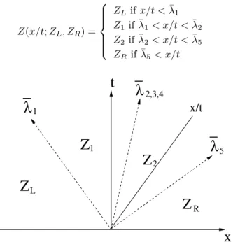
the linearized Riemann problem associated to J( ¯Z) and the states (ZR, ZL) is (see figure (10)),

Z(x/t; ZL, ZR) = ZL+ X ¯ λi<x/t αir¯i= ZR− X ¯ λi>x/t αi¯ri (44)

with:

¯

λi= λi( ¯Z) and r¯i= ri( ¯Z)

This can be written in a slightly different form:

Z(x/t; ZL, ZR) =          ZL if x/t < ¯λ1 Z1 if ¯λ1< x/t < ¯λ2 Z2 if ¯λ2< x/t < ¯λ5 ZR if ¯λ5< x/t

x

t

Z

Z

Z

Z

x/t

λ

λ

λ

−

−

−

Figure 10. The four different states of the solution of the linearized Riemann problem

We set ∆Φ = ΦR− ΦL. If we apply the formula (44) we find that the two intermediate states are:

Z1=         CL ρL+∆P_2¯a2 − ¯ ρ∆U 2¯a ¯ U −∆P2 ¯ρ¯a ¯ P − ¯ρ¯a∆U₂ YL         Z2=         CR ρR−∆P_2¯a2 − ¯ ρ∆U 2¯a ¯ U −∆P2 ¯ρ¯a ¯ P − ¯ρ¯a∆U₂ YR        

In the above formulas ¯a is the sound speed calculated at the average state ¯Z, that is ¯a = a( ¯Z). The numerical flux for the classical VFRoe-ncv scheme is computed using Z∗ _{= Z(x/t = 0; Z}

L, ZR) (for example in the

configuration of the figure (10) Z∗_{= Z} 1).

Remark. _{• The classical VFRoe-ncv scheme using variables (ρ, U, P ) for the HEM model (22):} The linear Riemann Problem associated to the system (22) has two intermediate states as shown in figure (10). The intermediate states are:

Z1=    ρL+_2¯a∆P2 H EM − ¯ ρ∆U 2¯aH EM ¯ U −2 ¯ρ¯a∆PH EM ¯ P − ¯ρ¯aHEM∆U₂    Z2=    ρR−_2¯a∆P2 H EM − ¯ ρ∆U 2¯aH EM ¯ U −2 ¯ρ¯a∆PH EM ¯ P − ¯ρ¯aHEM∆U₂   

• The classical VFRoe-ncv scheme using variables (C, ρ, U, P ) for the HRM model (4): The linear Rie-mann Problem associated to the system (4) has two intermediate states as shown in figure (10). The intermediate states are:

Z1=       CL ρL+_2¯a∆P2 H RM − ¯ ρ∆U 2¯aH RM ¯ U −2 ¯ρ¯a∆PH RM ¯ P − ¯ρ¯aHRM∆U₂       Z2=       CR ρR−_2¯a∆P2 H RM − ¯ ρ∆U 2¯aH RM ¯ U −2 ¯ρ¯a∆PH RM ¯ P − ¯ρ¯aHRM∆U₂      

C. A modified VFRoe-ncv scheme for the interface model

This modified VFRoe-ncv scheme for the interface model differs from the classical VFRoe-ncv scheme in the choice of the average state which is not a classical average. We use here the ”average state”:

˜

Z>= ( ¯C, ¯ρ, ¯U , ¯P , ˜Y ); Y =˜ (

0 if ¯U > 0 1 if ¯U < 0 This implies that the sound speed ¯a = a( ¯P , ¯ρ, ¯C, ¯Y ) is replaced by,

˜ a =

(

aHEM( ¯P , ¯ρ) if ¯U > 0

aHRM( ¯P , ¯ρ, ¯C) if ¯U < 0

This provides a new solution Z#_{(note that Y}#_{= ˜Y ). If we then explicit the numerical flux we find:}

F (Z#₎>_{= ((ρU C)}#_{, (ρU )}#_{, (ρU}2_{+ P )}#_{, (U (ρe(P, ρ, C, Y ) + ρU}2_{/2 + P ))}#_{, (ρU Y )}#₎

with,

e#= (

eHEM(P#, ρ#) if ¯U > 0

eHRM(P#, ρ#, C#) if ¯U < 0

Eventually, if ¯U > 0, this is equivalent to apply the VFRoe-ncv scheme to the HEM system (31) with in addition the equations on Y and C of (32); if ¯U < 0, this is equivalent to apply the VFRoe-ncv scheme to the HRM system (4) with in addition the equation on Y of (32).

VIII.

Appendix 2: Computation of C

and P

for

the finite time relaxation step

In order to compute the finite relaxation step we need to explain how Cn+1and Pn+1are updated. They are the solution at the time ∆t of the system (ODE) composed by the first and fourth equations of (40) with the initial condition: C(t = 0) = Cnˆ _{and P (t = 0) = P}nˆ_.

The main time step ∆t is cut into N small uniform time steps δt = ∆t/N. In the following Ciand Pi will

stand for the successive approximations of C and P at the successive times t = i × δt. Thus we will have: C0:= Cnˆ and P0:= Pˆn

Cn+1_{:= C}

N and Pn+1:= PN

The chain rule which provides (Ci+1, Pi+1) in terms of (Ci, Pi) is the following:

• Ci+1 is the exact solution at the time t = δt of the ODE system:

( d dtC(t) = Γ(Pi, ρ ˆ n_{, C(t))} C(t = 0) = Ci (45) where we have, Γ(Pi, ρnˆ, C(t)) = (1 − C(t)) ¡ Ceq(Pi, ρnˆ) − C(t) ¢ 1 Θ(Pi, ρnˆ, τ0)

with the time scale,

Θ(P, ρ, τ0) =

τ0

G2(P, ρ)

(46) where G2 defined by equation (18). We impose that the numerical approximation Ci+1 respects the

relations:

(Ci+1− Ceq(Pi, ρˆn))(Ci− Ceq(Pi, ρnˆ)) > 0 (47)

(1 − Ci+1)(1 − Ci) > 0 (48)

This relation corresponds to the fact that the analytical solution C(t) of (45) can not cross the poles C = Ceq(Pi, ρˆn) and C = 1.

We get Ci+1= Ci if Ci= 1 and if Ci6= 1,

Ci+1= bi+1+ Ceq(Pi, ρnˆ) 1 + bi+1 (49) with: bi+1= Ci− Ceq(Pi, ρnˆ) 1 − Ci e(ai+1δt) ₍₅₀₎ ai+1= −(1 − Ceq(Pi, ρnˆ)) G2(Pi, ρˆn) τ0 (51) • To compute Pi+1, we use the fourth equation of the system (40) in the form

∂t(P ) = −(∂P(eHRM))−1∂C(eHRM) ∂t(C)

and we make a rough integration:

Pi+1= Pi+ δt(∂t(P ))(Pi, ρnˆ, Ci+1, Ynˆ) that is: Pi+1= Pi− (Ci+1− Ci) µ ∂C(eHRM) ∂P(eHRM) ¶ (Pi, ρˆn, Ci+1, Ynˆ)

A numerical maximum principle :

We assume that Ceq(Pi, ρnˆ) remains in [0, 1].

• We assume that 0 ≤ Ceq(Pi, ρnˆ) ≤ Ci≤ 1 :

This implies that bi+1≥ 0. Hence using the equation (49) we get:

0 ≤ Ci+1≤ 1

• We assume that 0 ≤ Ci≤ Ceq(Pi, ρˆn) ≤ 1 :

This implies that bi+1≤ 0. We set,

H(b) = b + Ceq(Pi, ρ

ˆ n₎

1 + b and J(b) = 1 − H(b)

Thus we have H(bi+1) = Ci+1 and J(bi+1) = 1 − Ci+1. When we examine the positivity of both H(b)

and J(b) we find that it is equivalent to the relation b ≥ −Ceq(Pi, ρnˆ). This leads to the condition on

the time step δt:

δt ≥ 0 which is obviously fulfilled.

Hence we get for δt ≥ 0:

0 ≤ Ci+1≤ 1

We thus have the following property. Property:

The following maximum principle holds for the finite time relaxation step. If we assume that:

(i) the time step δt is positive,

(ii) the pole Ceq(Pi, ρˆn) of the ODE system (45) remains in [0, 1],

(iii) 0 ≤ Ci≤ 1

Then we have 0 ≤ Ci+1 ≤ 1.

Remark. Actually, the only assumption is that Ceq(Pi, ρnˆ) remains in [0, 1]. The finite time relaxation step

IX.

Appendix 3: On the discrete preservation of contact waves in HEM and

HRM models

A. HRM

This paragraph is strongly connected with the section dealing with the numerical schemes. It refers to the work exposed in.14 _{We formally set Γ = 0 in the system (4). A pure contact solution is an analytical solution}

of (4) (with Γ = 0) of the form: _         C(x, t) = C0(x − U0t) ρ(x, t) = ρ0(x − U0t) U (x, t) = U0 P (x, t) = P0 (52)

When the initial condition is such that the pressure and the velocity are uniform, the initial profiles of C and density (i.e. C0(x) and ρ0(x)) are advected with speed U0. We say that the contact solution is preserved by

the conservative numerical scheme if the numerical approximations of the velocity and the pressure remain constant in each cell of the discrete domain.

According to,14 _{the discrete contact solution is respected if two conditions are fulfilled:}

(i) The internal energy must be of the form:

ρe = f1(P ) + ρf2(P ) + ρCf3(P ) (53)

(ii) The numerical flux involved in the conservative scheme preserves the contact solution.

Remark. The second point (ii) is achieved when using either the Godunov scheme or VFRoe-ncv scheme with variables (C, ρ, U, P ).

The two conditions are necessary to preserve the discrete profiles of both U and P . If (i) is not fulfilled, the contact solution will not be respected whatever the conservative numerical scheme is (even for the Godunov scheme). We insist that whatever the continuous function defining the EOS (i.e. (P, ρ, C) 7→ eHRM(P, ρ, C))

for the HRM model is, the vector (52) is an analytical solution of the system (4) without any source term. Rewriting (12) we find that the internal energy is of the form:

ρe = φ1(P ) + ρφ2(P ) + ρC(−φ2(P )) (54) with: φ1(P ) = (δl− 1)P φ2(P ) = · (1 −_δδl v )hsv(P ) ¸

Hence this internal energy allows the discrete preservation of the contact wave since the condition (i) is fulfilled. In our numerical tests the convective part of the HRM model will be computed using a VFRoe-ncv scheme with variables (C, ρ, U, P ) that fulfills the condition (ii) (see14_).

B. HEM

The internal energy of the HEM model takes the form:

ρe = φ4(P ) + ρφ5(P ) (55)

with:

• In the pure liquid domain Dl:

• In the two-phase domain D2Φ: φ4(P ) = · −P +h s v(P ) − hsl(P ) τs v(P ) − τls(P ) ¸ φ5(P ) = · τs v(P )hsl(P ) − τls(P )hsv(P ) τs v(P ) − τls(P ) ¸

Following,14_{we conclude that this EOS allows the preservation of the discrete contact solution in the pure}

HEM domain. Hence when the discrete contact solution evolves in a single domain (i.e. in the pure liquid or in the two-phase domain), it is preserved provided that the numerical scheme preserves the contact solution. This is no longer true when going through the boundary between the domains D2Φ and Dl (a numerical

example is available in27_{). Once again, we recall that the convective part of the HEM model is computed}

using a VFRoe-ncv scheme with variables (ρ, U, P ). Hence, the condition (ii) is guaranteed (see14_).

C. Contact waves travelling through the coupling interface

We know that the discrete contact solutions are preserved by the HEM and the HRM models. We examine herein what happens when a contact wave hits the coupling interface (as described by figure (11)).

x

U

P

C (P , )

ρ

ρ

U

P

ρ

C

= C

x=0

HRM

HEM

Figure 11. Initial data for a contact test case hitting the coupling interface

Remark. Thanks to the preservation of the contact wave for sole HEM and HRM models, we only need to examine the discrete values of the variables in the two cells on each side of the coupling interface.

a ) U0> 0

A problem may only occur in the first cell in the HRM domain. After one time step of our coupling scheme involving VFRoe-ncv scheme and described above in appendix 1, we get in the first cell of the HRM domain the values (ρ, U, P, C) defined by:

ρ − ρR+ λ(ρRU0− ρLU0) = 0 (56)

ρU − ρRU0+ λ(ρRU02+ P0− ρLU02− P0) = 0 (57)

ρEHRM− ρREHRMR + λ(U0(ρREHRMR + P0) − U0(ρLEHEML + P0)) = 0 (58)

ρC − ρRCR+ λ(ρRU0CR− ρLU0CeqL) = 0 (59) with λ =_∆x∆t and: EHRM = eHRM(P, ρ, C) + U2 2 ER HRM = eHRM(P0, ρR, CR) + U2 0 2

ELHEM = eHEM(P0, ρL) + U2 0 2 = eHRM(P0, ρL, C L eq) + U2 0 2 CeqL = Ceq(P0, ρL)

Using the internal energy in the form (54), the system (56)-(59) provides:

ρ − ρR+ λU0(ρR− ρL) = 0 (60)

U = U0 (61)

(Φ1(P ) − Φ1(P0)) + ρ(1 − C)(Φ2(P ) − Φ2(P0)) = 0 (62)

ρC − ρRCR+ λ(ρRU0CR− ρLU0CeqL) = 0 (63)

The equation (62) implies that for any ρ ≥ 0 and for any ρ(1 − C) ≥ 0 defined by (60) and (63): Φ1(P ) = Φ1(P0) and Φ2(P ) = Φ2(P0)

and thanks to the bijectivity of the applications P 7→ Φ1(P ) and P 7→ Φ2(P ) this leads to P = P0.

Thus the contact wave passing from the HEM model to the HRM model will be preserved. b ) U0< 0

A problem may only occur in the first cell in the HEM domain. One time step of the coupling described above provides in the first cell of the HEM domain the values (ρ, U, P ) defined by:

ρ − ρL+ λ(ρRU0− ρLU0) = 0 (64)

ρU − ρLU0+ λ(ρRU02+ P0− ρLU02− P0) = 0 (65)

ρEHEM− ρLEHEML + λ(U0(ρREHRMR + P0) − U0(ρLEHEML + P0)) = 0 (66)

with λ =_∆x∆t and: EHEM = eHEM(P, ρ) +U 2 2 EHRMR = eHRM(P0, ρR, CR) +U 2 0 2 EHEML = eHEM(P0, ρL) +U 2 0 2 Using the internal energy in the form (55), the system (64)-(66) provides:

ρ − ρL+ λ(ρRU0− ρLU0) = 0 (67)

U = U0 (68)

Φ4(P ) − Φ4(P0) + ρ(Φ5(P ) − Φ5(P0)) + λU0ρR(eRHRM− eRHEM) = 0 (69)

Hence if P = P0 , the equation (69) reads:

eHRM(P0, ρR, CR) = eHRM(P0, ρR, CeqR)

which thanks to the bijectivity of C 7→ eHRM(P, ρ, C) implies that CR = CeqR. Then a necessary condition

for the respect of the discrete contact solution is:

CR= Ceq(P0, ρR)

Let us now assume that CR= Ceq(P0, ρR). Thus eHRM(P0, ρR, CR) = eHRM(P0, ρR, CeqR), and the pressure

P is a solution of the equation: