Modelling and thermal analysis of a seismic borehole sensor : diploma 2015

Texte intégral

(1)Degree Programme Systems Engineering Major Power & Control. Diploma 2015 Yves Ravedoni Modelling and thermal analysis of a seismic borehole sensor. Professor Dr . D et l ef R e d lic h Expert Dr . J os e ph Mo er s c he l l Submission date of the report 04 . 09 .2 0 15.

(2) This document is the original report written by the student. It wasn’t corrected and may contain inaccuracies and errors..

(3)

(4) Modelling and thermal analysis of a seismic borehole sensor Graduate. Ravedoni Yves. Objectives Analysis and adaptation of an acquisition system for a seismometer to enable operation at high temperatures (up to 180 [°C]). The simulation software and thermal measurements are used to validate theoretical results.. Methods | Experiences | Results. Bachelor’s Thesis | 2015 |. Degree programme Systems Engineering. This thesis has been prepared in Jena, in Germany, as part of an exchange. The first step entails studying an existing sensor. Thermal measurements are performed. The temperature of components is established, it will confirm that the components work within a correctly prescribed operational temperature range. The measured environment is created by FEM thermal simulation software. The results are compared and simulation parameters are adjusted so that the simulation results correspond to the reality. For the second step, the housing of the sensor is altered to be placed in a borehole at a temperature of 180 [°C], a pressure of 25 [bar] and a depth of 3 [km]. The design of the printed circuit board is analysed, the electronic components are selected to operate at the required temperatures. Thermal simulation is used to certify that each component does not exceed the prescribed maximum operating temperature. The “graphite heat spreader” and “Peltier” elements (thermoelectric cooler) are studied whilst seeking to improve results.. Field of application Major Power & Control. Supervising Professor Dr. Detlef Redlich Detlef.redlich@fh-jena.de. Expert Professor Dr. Joseph Moerschell Joseph.moerschell@hevs.ch. Partner Fachhochschule Ernst-Abbe Hochschule Jena - Deutschland Thermal simulation on the PCBs of the existing sensor. The ambient temperature is 25 [°C]. Without housing.. Infrared picture of the existing sensor in its housing. The ambient temperature is 25.5 [°C]. ε=0.9.

(5) Systems Engineering Power and Control – Bachelor thesis Thermal analysis of a seismic borehole sensor. TABLE OF CONTENTS I. II.. GENERAL SPECIFICATIONS ................................................................................................. 3 INTRODUCTION ...................................................................................................................... 4. 1. 2.. OBJECTIVES .......................................................................................................................................... 4 AIM OF A SEISMIC SENSOR ................................................................................................................. 4 2.1 GENERAL ASPECTS ..................................................................................................................... 4 2.2 BOREHOLE .................................................................................................................................... 5 3. ENVIRONMENT ...................................................................................................................................... 5. III.. RESEARCH ON EXISTING SENSOR ..................................................................................... 6. 1.. OVERVIEW ............................................................................................................................................. 6 1.1 BACKGROUND .............................................................................................................................. 6 1.2 ELECTRICAL SCHEMATICS ......................................................................................................... 7 1.3 THERMAL CHARACTERISTICS .................................................................................................... 7 1.4 POWER DISSIPATION ................................................................................................................... 9 1.4.1 TEMPERATURE OF COMPONENTS ........................................................................................ 9 1.4.2 HEAT SOURCES ..................................................................................................................... 12 1.4.3 POWER DISSIPATION ON EXISTING SENSOR .................................................................... 12 THERMAL MEASUREMENTS .............................................................................................................. 13 2.1 RESISTIVE SENSOR ................................................................................................................... 14 2.2 INFRARED CAMERA ................................................................................................................... 15 2.2.1 CAMERA 1 ............................................................................................................................... 15 2.2.2 CAMERA 2 ............................................................................................................................... 17 2.3 RESULTS ANALYSIS ................................................................................................................... 20 SIMULATIONS ...................................................................................................................................... 22 THERMAL STATIC SIMULATIONS....................................................................................................... 23 FLOW SIMULATIONS ........................................................................................................................... 24 5.1 SIMPLIFICATION ......................................................................................................................... 25 5.2 SPECIFICATIONS ........................................................................................................................ 26 5.3 RESULTS ..................................................................................................................................... 27 COMPARISON BETWEEN THERMAL MEASUREMENTS AND SIMULATION RESULTS ................. 30 6.1 IMPROVEMENTS ......................................................................................................................... 31. 2.. 3. 4. 5.. 6.. IV.. REALIZATION ........................................................................................................................ 33. 1.. OBJECTIVES AND CRITERIA .............................................................................................................. 33 1.1 ENVIRONMENT AND CONDITIONS ........................................................................................... 33 1.2 MECHANICAL DESIGN ................................................................................................................ 35 1.3 TEMPERATURE CONDITIONS ................................................................................................... 36 1.4 ELECTRONIC CONCEPTION ...................................................................................................... 36 1.5 ELECTRICAL DIAGRAM AND COMPONENTS ........................................................................... 37 2. VARIANT 1 ............................................................................................................................................ 38 2.1 ELECTRONIC COMPONENTS .................................................................................................... 38 2.2 MECHANICAL DESIGN ................................................................................................................ 38 2.3 SPECIFICATIONS OF SIMULATION ........................................................................................... 40 2.4 RESULTS ..................................................................................................................................... 41 2.5 COST AND IMPROVEMENTS ..................................................................................................... 43 3. VARIANT 2 ............................................................................................................................................ 43 3.1 ELECTRONIC COMPONENTS .................................................................................................... 43 3.2 PELTIER ELEMENT ..................................................................................................................... 44 3.3 MECHANICAL DESIGN ................................................................................................................ 45 3.4 SPECIFICATIONS OF SIMULATION ........................................................................................... 46 3.5 RESULTS ..................................................................................................................................... 47 3.6 IMPROVEMENTS ......................................................................................................................... 51 4. ANALYSIS ............................................................................................................................................. 53 4.1 PERFORMANCE OF MODELS .................................................................................................... 53 4.2 COST ............................................................................................................................................ 53 4.3 IMPROVEMENTS ......................................................................................................................... 54. V. VI. VII.. CONCLUSION ........................................................................................................................ 55 THANKS ................................................................................................................................. 56 DATE ET SIGNATURE .......................................................................................................... 57. Jena, 04 September 2015. 1/61. Yves Ravedoni.

(6) Systems Engineering Power and Control – Bachelor thesis Thermal analysis of a seismic borehole sensor VIII. IX. X. XI.. INDEX OF ANNEXES ............................................................................................................ 58 INDEX OF FIGURES.............................................................................................................. 59 INDEX OF TABLES ................................................................................................................ 60 BIBLIOGRAPHY ..................................................................................................................... 61. Jena, 04 September 2015. 2/61. Yves Ravedoni.

(7) Systems Engineering Power and Control – Bachelor thesis Thermal analysis of a seismic borehole sensor. I.. GENERAL SPECIFICATIONS. List of the tasks undertaken during this thesis: . Mastering of Ansys Workbench, Ansys “Icepak”, Pcad, CoCreat software. . Simulation and measurement of power dissipation on an existing sensor. . Temperature measurement on the existing sensor and the components. . Thermal simulation on the existing sensor. . Researching components for the new sensor. . Analysing different circuit board designs. . Simulating the new sensor in different temperatures and specifications. . Thesis documentation. . Preparation of an “oral defence” of the thesis. Jena, 04 September 2015. 3/61. Yves Ravedoni.

(8) Systems Engineering Power and Control – Bachelor thesis Thermal analysis of a seismic borehole sensor. II.. INTRODUCTION 1. Objectives. The aim of the work is to present two seismic sensors that work in high temperatures (70°C and 150°C). This implies resolving the problem by seeking electronic devices and PCB designs that will work in harsh conditions. General components have a maximal temperature of 85°C. Durability cannot be certified the when the electronics are used at temperatures over 85°C. There are three options to provide a solution to problems caused by high temperatures: . Different Printed Circuit Board (PCB) design. . Cooling systems (static or dynamic). . Use of High temperature electronics.. A thermal simulation analysis is made to know the temperatures of each of the components. This will help to prevent any temperature damage of the sensor and will improve the reliability, giving a good performance. To start with, an existing sensor is analysed.. 2. Aim of a seismic sensor 2.1 General aspects A seismic sensor is built to measure earth movements, such as earthquakes. These vibrations have low frequencies, from 2 to 100 Hz. There are three categories of movement sensors. . Seismometers, made with a complex mechanism, is designed for low frequency measurements. The disadvantage is their big size and their fragility.. . Geophones, made with a magnet in a coil. They are optimised for low frequencies (4400Hz). These sensors are generally used to measure seismic waves or vibrations on industrial machines.. . Accelerometers, made to measure acceleration amplitudes rather than movement waves. They can be built into integrated circuits.. In this thesis, geophones sensors are used because they are smaller, more practical and less fragile than seismometers and more performant than accelerometers for seismic measures. Three sensor are used to measure the three axis.. Jena, 04 September 2015. 4/61. Yves Ravedoni.

(9) Systems Engineering Power and Control – Bachelor thesis Thermal analysis of a seismic borehole sensor 2.2 Borehole The aim of this “seismic borehole sensor” is to provide a constant monitoring of seismic waves activity, and reveal the earthquake movements for general seismic database. The new seismic sensor is designed to make measurements in boreholes. This is a static measure; the sensor is physically placed at the bottom of the borehole and left there for many years. Borehole seismic measurements provide precise values (less signal noise) and quicker seismic results than earth surface sensors. This is because with depth there is more rocks and a bigger density that bring a better signal.. 3. Environment These are the constraints due to depth in a borehole are: . High temperature. . Dust and water. . High pressure. . Size constraints. . Power supply and data transfers. The general geothermal average gradient is about 25 [°C/km] (Analog Device, technical article MS-2707). For this thesis, environment values were given. The first variant has an environment temperature Tnominal = 150 [°C] and a maximal environment temperature of T max=180 [°C]. The maximal depth is 3 [km] long and the pressure is P=24 [bar]. The second variant has an environment temperature Tnominal = 75 [°C] and a maximal environment temperature of Tmax=100 [°C]. The maximal depth is 1km long and the pressure is P=24 [bar].. Jena, 04 September 2015. 5/61. Yves Ravedoni.

(10) Systems Engineering Power and Control – Bachelor thesis Thermal analysis of a seismic borehole sensor. III.. RESEARCH ON EXISTING SENSOR 1. Overview 1.1 Background. The existing seismic sensor is the “semester” work of three colleagues. Their aim was to develop and create a seismic sensor that measures low frequency movement in 3 directions from the ground or a building. Values are filtered and saved before they are sent to a general server. The server is able to show values of different sensors.. Figure 1 Existing sensor, when it is open. This seismic sensor is made with general electronic components. Three geophones measure linear displacement. The first PCB board contains an analogue signal treatment component, analogue/digital converter component, and power units. The second PCB is a “Raspberry PI B+” microcomputer used to collect measured values and send them to a computer via a wireless connexion. The housing is made from ABS plastic printed on a 3D printer. Choices were made to have a sensor that is able to obtain values, send them, and show them on a screen. Because of lack of time, precision and optimisation are limited.. Jena, 04 September 2015. 6/61. Yves Ravedoni.

(11) Systems Engineering Power and Control – Bachelor thesis Thermal analysis of a seismic borehole sensor 1.2 Electrical schematics The following diagram shows the electronic structure. The scheme is in annexe 1. Power Supply. DC LDO. Converter. Oscillator. DC DC. A. X. Computer Device. Y. Z Geophones. D. Operational Amplifiers. Analog/ Digitial Converter. Processor. Wireless transmitter. Figure 2 Existing sensor, electronic diagram1. For each axis (X, Y and Z), the input signal coming from the geophone goes to a fully differential operational amplifier and is then filtered. All three signals are then digitised through an analogue/digital converter. With a SPI interface, measured data are transferred to the “Raspberry PI” processor. The processor sends data wirelessly to the connected server. The power is supplied by a 5V LDO (Low DropOut regulator) and a DC/DC converter that creates a -5V. An oscillator is also needed for the sampling frequency of the AD converter. The components on the PCB are represented on the following picture.. 1.3 Thermal characteristics The Table 1 shows the maximal temperature of the used components. Their Datasheets can be found in annexes 4-7.. 1. Inspired by report „Reseau de capteur sismiques“, Thomas Oggier, Yannick Dayer et Fabien Clerc, 04/09/2014. Jena, 04 September 2015. 7/61. Yves Ravedoni.

(12) Systems Engineering Power and Control – Bachelor thesis Thermal analysis of a seismic borehole sensor Type Geophone Operational amplifier Analogue/digital converter Processor Wireless device DC/DC converter 5V LDO Oscillator Resistor & Capacitor. Component name GS-11D OPA1632 ADS1254 BCM2835 ARM TEW-648UBM TMC 0505D ADP3338 TXC 7C General SMD. Maximal temperature [°C] 100 85 85 85 85 85 85 85 85. Table 1 Existing sensor, maximal temperature of components. The maximal given temperature is that of the components and not that of the environment. More details are explain in the chapter III.1.4.1. The components on the PCB are represented on the following pictures.. Figure 3 Real PCB of the existing sensor. Jena, 04 September 2015. 8/61. Yves Ravedoni.

(13) Systems Engineering Power and Control – Bachelor thesis Thermal analysis of a seismic borehole sensor. 3x OP amplifier. A/D converter. DC/DC converter. LDO Processor. Usb processor. Figure 4 Simplified PCB of the existing sensor. 1.4 Power dissipation The heat source value of each component is called power dissipation. It’s related to the losses of components due to their efficiency. Power dissipation value is needed to calculate the temperature that every component reaches.. 1.4.1 Temperature of components The “thermal flow resistive diagram” is a way to know the temperature of components. It can be calculated using the value of power dissipation, thermal resistivity and environment temperature. In general, a representation of the thermal flow is made in correlation with an electrical circuit. The correlations are the followings: Power dissipation ~ Current. Pd [W] ~ I. Delta temperature ~ Voltage. ∆θ [°C] ~ U. 1. Thermal resistor ~ 𝑇ℎ𝑒𝑟𝑚𝑎𝑙 𝑐𝑜𝑛𝑑𝑖𝑐𝑡𝑖𝑣𝑖𝑡𝑦 = resistor. ∆θ. 1. °𝐾. 𝑅 = 𝑃𝑑 = 𝜆 = [ 𝑊 ]. The Figure 5 shows the thermal flow diagram of a component into a housing. This representation will help to visualise the heat flow from a component, which dissipates its heat to the environment.. Jena, 04 September 2015. 9/61. Yves Ravedoni.

(14) Systems Engineering Power and Control – Bachelor thesis Thermal analysis of a seismic borehole sensor θin. θout. θb. Pd. Rhi_rad. Rb_rad. Rh. Rho_rad. Pd Rb. Rb_conv. θin. Rhi_conv. Rho_conv. θb. Conductivity. Radiation + Convection. θout. Inside Radiation + Convection. Conductivity. Electronic componant. Outside Radiation + Convection. Housing wall. Figure 5 Thermal flow from an electronic heat source through a housing to environment. To simplify comprehension, only one direction of the thermal flow is showed on Figure 5. To find the temperature of the component θin and inside the housing θb, its use the power dissipation value, the thermal resistances and the environment temperature. A computer works the same way, but it calculates the whole environment to have more exact values. Every material has an inner thermal resistance (opposite of thermal conduction). Unit are in [W *mm-1*K-1]. For example, ABS = 0,15-0,3 [W*mm-1*K-1] and Epoxy = 0,3-10 [W *mm-1*K-1]. On every surface there is convection and radiation, always represented in parallel. Here is usual convection2 in [W *m-2*K-1] at 20 [°C] between . A body and free air. 2-25. . A body and a liquid. 50-1’000. . A body and a forced air flow. 25-250. . A body and a forced liquid flow. 50-20’000. . A body and a changing phase fluid. 2’500-100’000. 2. Data from script “Ansys tutorial, Für das Analyse-System Steady State Thermal und Komponentensystem Icepak” Prof. Dr. Detlef Redlich, 2011.. Jena, 04 September 2015. 10/61. Yves Ravedoni.

(15) Systems Engineering Power and Control – Bachelor thesis Thermal analysis of a seismic borehole sensor In this thesis, components have free air convection. The value is approximated at 5 [W *m-2*K-1]. Radiation value is between 0 and 1, and is unitless. When there is no radiation, ε=0. A body with maximal radiation is called a black body, and emission coefficient is nearly ε=1.. Material Epoxy Copper Gold PVC Solder mask. Emission coefficient 0,79 0,3 0,26 0,97 0,8. Table 2 Average emission coefficient for different materials in temperature of 22-150 [°C].3. With Radiation constant, Stefan-Boltzmann constant (σ=5,67*10-8 [W *m-2*K-4]), and the environment temperature, the surface conductivity can be calculated. 𝜀. 𝐻𝑟𝑎𝑑𝑖𝑎𝑡𝑖𝑜𝑛 = 4 ∙ 𝜀−1 ∙ 𝜎 ∙ 𝑇𝑎𝑚𝑏𝑖𝑒𝑛𝑡 3 [W*m-2*K-1] Equation 1 4. Conductivity, convection and radiation are dependent on the environment temperature. For example, equation 2 and 3 show that a ceramic component (ε=0.9) will have a surface conductivity of 51,3 [W *m-2*K-1] at 20 [°C] and 154,5 [W*m-2*K-1] at 150 [°C]. 0.9. 𝐻𝑟𝑎𝑑𝑖𝑎𝑡𝑖𝑜𝑛,20 = 4 ∙ 1−0.9 ∙ 𝜎 ∙ 2933 = 51,3 [W*m-2*K-1] Equation 2. 0.9. 𝐻𝑟𝑎𝑑𝑖𝑎𝑡𝑖𝑜𝑛,150 = 4 ∙ 1−0.9 ∙ 𝜎 ∙ 4233 = 154,5 [W*m-2*K-1] Equation 3. Radiation increases exponentially with the ambient temperature. Equation 4 and 5 are with the same temperature but a smaller emission coefficient (ε=0.5). 0.5. 𝐻𝑟𝑎𝑑𝑖𝑎𝑡𝑖𝑜𝑛,20 = 4 ∙ 1−0.5 ∙ 𝜎 ∙ 2933 = 5,7 [W*m-2*K-1] Equation 4. 0.5. 𝐻𝑟𝑎𝑑𝑖𝑎𝑡𝑖𝑜𝑛,150 = 4 ∙ 1−0.5 ∙ 𝜎 ∙ 4233 = 17,2 [W*m-2*K-1] Equation 5. 3. Data from script “Ansys tutorial, Für das Analyse-System Steady State Thermal und Komponentensystem Icepak” Prof. Dr. Detlef Redlich, 2011. 4 Equation from script „Systemes Energetiques - Thermodynamique“ Michel Bonvin et Jessen Page, 2015. Jena, 04 September 2015. 11/61. Yves Ravedoni.

(16) Systems Engineering Power and Control – Bachelor thesis Thermal analysis of a seismic borehole sensor With an emission coefficient (ε=0.5), the surface conductivity is 5,7 [W *m-2*K-1] at 20 [°C] and 17,2 [W *m-2*K-1] at 150 [°C]. In comparison, the radiation has a bigger surface conductivity than convection.. 1.4.2 Heat sources For the simulation, not all electronic components are taken into consideration. The analysis is only made with the main heat sources, such as the operational amplifier, the analogue/digital converter, the processor and the power supply. In equation 6, a resistor of 1 [kΩ] with 5 [V] alimentation has only 25 [mW] of power which is 100 [%] power dissipation (active component).. 𝑈2 52 𝑃𝑑 = 𝑃 = = = 25 [𝑚𝑊] 𝑅 1000 Equation 6. Pd = 25 [mW] is an insignificant small value, it doesn´t have a big impact on the thermal analysis. Because all the resistors produce less power than 25 [mW], these have not been taken into consideration. Capacitors are passive components, so they don’t have any power dissipation.. 1.4.3 Power dissipation on existing sensor In basic components, power consumption and power dissipation are not necessarily in the datasheet. This is the case for components in Table 1. The power consumption of each component can be found by simulating the circuit. Unfortunately no corresponding components (OPA1632 and ADS1254) were working on OrcadPcad (the software employed). The LME49724 is an alternative operational amplifier that worked on Pcad, but power results were false (10 MW). The last solution for this existing sensor is to measure on the PCB the voltage and the current, where it’s possible, to define a power consumption. A percentage of this consumption is approximated as dissipation power.. Power measurement and estimation : Power green PCB Processor USB-processor Power yellow PCB 3 OPamplifier 1 OPamplifier AD converter DC/DC Converter. Pnom [mW]. Pmax [mW]. 1342,74 850 392,74 977,92 780 260 100 97,92. 1542,1 976,2 465,9 997,3 789,4 263,1 105,0 102,8. % off Power dissip.. Pdiss,min [mW]. Pdiss,max [mW]. 90% 90%. 765,0 353,5. 878,6 419,3. 80% 80% 90% 28%. 624,0 208,0 90,0 27,4. 631,5 210,5 94,5 28,8. Table 3 Existing sensor, power consumption and dissipation estimation. Jena, 04 September 2015. 12/61. Yves Ravedoni.

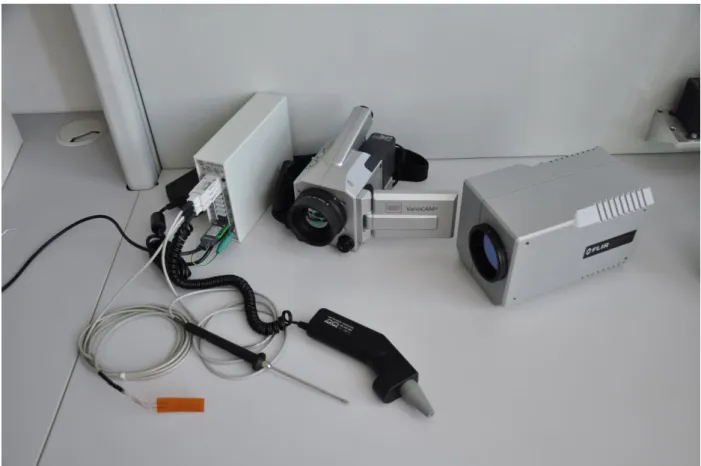
(17) Systems Engineering Power and Control – Bachelor thesis Thermal analysis of a seismic borehole sensor All the components are welded so it is only possible to measure the current and the power of each PCB. These measured values are in red. This power is divided between the components on the PCB, orange values (approximation). According to the efficiency of each component an approximation of power dissipation is made. These values are adjusted with simulation results to make them correspond with real temperature measurements.. 2. Thermal measurements Temperature measurements are made on the existing sensor. The values of major heating sources are measured. These temperatures are useful to compare and certify that simulation results are correct. Three different measurement units are used.. Figure 6 Temperature measurement devices. Summary of the thermal measurement campaign: 1. Values measured with resistive sensor and thermal paste 2. First infrared camera values, only maximal values can be measured 3. Second infrared camera, maximal and average values. Measure when PCB is in and out of the housing.. Jena, 04 September 2015. 13/61. Yves Ravedoni.

(18) Systems Engineering Power and Control – Bachelor thesis Thermal analysis of a seismic borehole sensor 4. Processor temperature with PT100 sensor and thermal paste. When PCB is in the housing. 5. Comparison between obtained maximal values 6. Comparison between average and maximal values (second camera). 2.1 Resistive sensor The “Ahlborn Almemo” unit is a data logger that works with different kind of sensors. Data logger values can be seen on a computer. The first contact probe has been used to measure the environment temperature and small components. The flat probe has been used for the Processor only, because other components are too small. Both sensors have a precision of +/- 0,1 [°C]. The following table shows the maximal measured temperature. This is made with PCB out of the housing. Other components are not accessible for thermal measures. Thermal paste is used to improve the contact between the sensor and the component. Even though thermal paste is present, error can be due to lack of the positioning precision and the thermal paste resistance.. Ambient OPA X OPA Y OPA Z AD TRACO. PT100 Contact Probe ZA 9030 FS1 [°C] 22,1. PT100 Contact Probe ZA 9030 FS1. Delta T (with ambient). [°C]. [°C]. 44,7 45,8 44,6 41,1 40,9. 22,6 23,7 22,5 19 18,8. Table 4 Measuring results of Almemo sensors. The Table 5 shows the temperature of the processor when the PCB is in a closed housing. The measure is made with thermal paste. The probe is the “PT100 Flat probe ZA 9030 FS1”.. Ambient Processor. PT100 PT100 Contact Flat Probe Probe ZA 9030 FS1 ZA 9030 FS1 [°C] [°C] 25,9 57,5. Delta T (with ambient) [°C] 31,6. Table 5 Processor temperature when running in closed housing. Jena, 04 September 2015. 14/61. Yves Ravedoni.

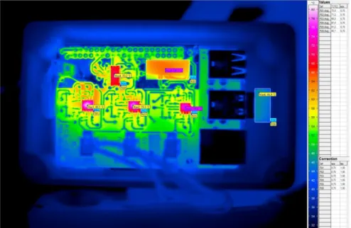
(19) Systems Engineering Power and Control – Bachelor thesis Thermal analysis of a seismic borehole sensor. 2.2 Infrared camera The infrared wavelength zone is from 700 nm to 1mm (visible is from 380-710 nm). Infrared cameras are designed to measure wavelengths in this range. Infrared radiation is treated and represented in human visible spectrum. A body emits and absorbs infrared wavelengths depending on its temperature and its surface material. By knowing the body surface material (coefficient of emissivity, epsilon ε) it is possible to know the temperature of the body (see chapter III.1.4.1 page 9). The two following chapters present infrared camera pictures with thermal results of the existing sensor. Here is a list of source of errors in the thermal measurements: . The set environment temperature is probably not exact. . The emission coefficient set on component zone is set as ε=0.6 or ε=0.7. It is not exact. It’s should be around 0.8< ε <0.9 for plastic or ceramic black components.. . Measures have not been taken in darkness. Environment reflexion can distort values.. 2.2.1 Camera 1 The Flir infrared camera is the first camera used. All values are with PCB out of the housing. In Figure 7 and Figure 8 are examples of thermal infrared acquisition with the Flir camera. The emission coefficient is set as ε=0.7.. Figure 7 Infrared thermal acquisition with Flir camera, with measuring points. ε=0.7. Jena, 04 September 2015. 15/61. Yves Ravedoni.

(20) Systems Engineering Power and Control – Bachelor thesis Thermal analysis of a seismic borehole sensor. Figure 8 Processor infrared thermal acquisition with Flir camera, with measuring points. ε=0.7. Maximal temperature. Ambient OPamp X OPamp Y OPamp Z AD conv. DC/DC conv. Geoph. X Geoph. Y Geoph. Z Processor Usb processor. Emission coefficient. Table 6 shows the measuring results.. Measuring points. Figure 7_SP01 Figure 7_SP02 Figure 7_SP03 Figure 7_SP04 Figure 7_SP05. Figure 8_SP01. 0,7 0,7 0,7 0,7 0,7 0,7 0,7 0,7 0,7. Infrared Camera Flir SC500 [°C] 25,8 58,9 61,9 66,2 54,8 48,7 29,9 25,8 25,8 55,4. Figure 8_SP02 0,7 45 Table 6 Measuring results of Flir camera. Delta T (with ambient) [°C] 33,1 36,1 40,4 29 22,9 4,1 0 0 29,6 19,2. Geophones are not heat sources, values are incorrect because of their steel housing. The steel has an emission coefficient of ε=0,3-0,5 so it disrupts the infrared sensor.. Jena, 04 September 2015. 16/61. Yves Ravedoni.

(21) Systems Engineering Power and Control – Bachelor thesis Thermal analysis of a seismic borehole sensor 2.2.2 Camera 2 “JenOptic” “VarioCAM” camera is a more recent camera and more powerful than the Flir camera. It’s more practical (runs on battery), it has a better resolution and functionality. The lens can be changed, and the software is powerful. Here is a picture during measurements.. Figure 9 JenOptic VarioCAM during measurements. The Figure 10 and Figure 11 are infrared pictures taken with the JenOptic VarioCAM camera. The general emission coefficient is ε=0.9. The plastic housing of the electrical components has an emission coefficient of ε=0.7, so each component’s zone is set to this value. In Figure 11 components are not perpendicular to the camera, a smaller emissivity of ε=0.6 is supposed.. Jena, 04 September 2015. 17/61. Yves Ravedoni.

(22) Systems Engineering Power and Control – Bachelor thesis Thermal analysis of a seismic borehole sensor. Figure 10 IR picture with VarioCAM, of existing sensor PCB just after being used in closed housing. Figure 11 IR picture with VarioCAM, Processor and USB processor when PCB running out of the housing. The following table shows the maximal temperature of components. With or without the housing, the delta T value is nearly the same (absolute error < 4,4°C).. Jena, 04 September 2015. 18/61. Yves Ravedoni.

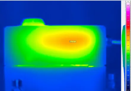
(23) Ambient Inside housing OPamp X OPamp Y OPamp Z AD conv. DC/DC conv. Geoph. X Geoph. Y Geoph. Z Processor Usb processor LDO Wifi device. Emission coefficient. Maximal temperature. Measuring points. Systems Engineering Power and Control – Bachelor thesis Thermal analysis of a seismic borehole sensor. _R03 _R02 _R01 _R04 _R05. 0,7 0,7 0,7 0,7 0,7 0,6 0,6 0,6 0,6 0,6 0,7 0,7. _X01 _X02. PCB outside housing PCB inside housing Infrared Infrared Delta T Camera Delta T Camera Delta T (with VarioCAM (with VarioCAM (with inside Obj. ambient) Obj. ambient) housing 1.0/30 1.0/30 temp) [°C] [°C] [°C] [°C] [°C] 25 25,5 37,5 12 61,9 36,9 75,8 50,3 38,3 63,5 38,5 78,3 52,8 40,8 63,2 38,2 80,1 54,6 42,6 53,8 28,8 70,2 44,7 32,7 52 27 64,7 39,2 27,2 28 3 30 4,5 -7,5 28 3 30 4,5 -7,5 28 3 30 4,5 -7,5 62,4 37,4 Can't be measured 45 20 Can't be measured 73,7 48,7 Can't be measured 35,4 10,4 46,9 21,4 9,4. Table 7 Maximal temperature measured with VarioCAM. Figure 12 shows a thermal preview of the housing. This shows that temperature is hotter in the housing. The housing has a bad thermal conductivity, because it does not have the same global temperature.. Figure 12 IR picture with VarioCAM, Preview of the housing temperature when sensor is working. ε=0.9. On the datasheet, the maximal operating temperature corresponds to the temperature of the package and not the Die. To compare the datasheets with the IR pictures, the average. Jena, 04 September 2015. 19/61. Yves Ravedoni.

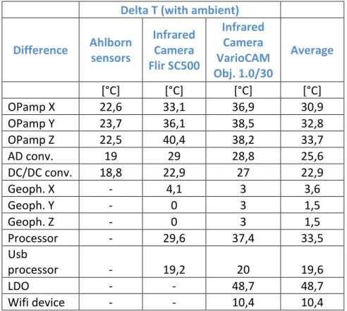
(24) Systems Engineering Power and Control – Bachelor thesis Thermal analysis of a seismic borehole sensor temperature of component’s zone (on IR picture) is used. Average measured temperatures are in Table 8. These two temperatures correspond also to the results given by simulation.. Ambient Inside housing OPamp X OPamp Y OPamp Z AD conv. DC/DC conv. Geoph. X Geoph. Y Geoph. Z Processor Usb processor LDO Wifi device. _R03 _R02 _R01 _R04 _R05. _X01 _X02. PCB inside housing. [°C] 25. [°C]. [°C] 25,5. [°C]. Delta T (with inside housing temp) [°C]. 0,7 0,7 0,7 0,7 0,7 0,6 0,6 0,6 0,6. 55,7 56,8 56,9 53,8 46,9 26 26 26 59,3. 30,7 31,8 31,9 28,8 21,9 1 1 1 34,3. 37,5 69,4 72,3 72,8 67 63 30 30 30 64,1. -21,4 43,9 46,8 47,3 41,5 37,5 4,5 4,5 4,5 38,6. 31,9 34,8 35,3 29,5 25,5 -7,5 -7,5 -7,5 26,6. 0,6 0,7 0,7. 44,6 56,5 33,5. 19,6 31,5 8,5. Can't be measured Can't be measured 44,1 18,6. Emission coefficient. Average temperature. Measuring points. PCB outside housing Infrared Camera VarioCAM Obj. 1.0/30. Delta T (with ambient). Infrared Camera VarioCAM Obj. 1.0/30. Delta T (with ambient). 6,6. Table 8 Average temperatures measured with VarioCAM. 2.3 Results analysis Table 9 is a comparison of maximal measured values from Alhlborn, Flir, JenOptic sensors. This is when the PCB is out of the housing.. Jena, 04 September 2015. 20/61. Yves Ravedoni.

(25) Systems Engineering Power and Control – Bachelor thesis Thermal analysis of a seismic borehole sensor. Difference. OPamp X OPamp Y OPamp Z AD conv. DC/DC conv. Geoph. X Geoph. Y Geoph. Z Processor Usb processor LDO Wifi device. Delta T (with ambient) Infrared Infrared Ahlborn Camera Camera sensors VarioCAM Flir SC500 Obj. 1.0/30 [°C] [°C] [°C] 22,6 33,1 36,9 23,7 36,1 38,5 22,5 40,4 38,2 19 29 28,8 18,8 22,9 27 4,1 3 0 3 0 3 29,6 37,4 -. 19,2 -. 20 48,7 10,4. Average [°C] 30,9 32,8 33,7 25,6 22,9 3,6 1,5 1,5 33,5 19,6 48,7 10,4. Table 9 Comparison between maximal sensors values, when PCB is out of housing.. Table 9 shows that there is a big difference between the sensors. To make improvements, the results should be studied and the specifications (emission coefficient, dissipation power) adjusted. With the JenOptic VarioCAM infrared values, the difference between maximal and average temperature is approximately 6 [°C].. Jena, 04 September 2015. 21/61. Yves Ravedoni.

(26) Systems Engineering Power and Control – Bachelor thesis Thermal analysis of a seismic borehole sensor PCB outside housing Infrared Camera VarioCAM Obj. 1.0/30. PCB inside housing. Average temperature. Maximal temperature. [°C] 25. [°C] 25. 55,7 56,8 56,9 53,8 46,9 26 26 26 59,3. 61,9 63,5 63,2 53,8 52 28 28 28 62,4. 6,2 6,7 6,3 0 5,1 2 2 2 3,1. 44,6 56,5 33,5. 45 73,7 35,4. 0,4 17,2 1,9. Ambient Inside housing OPamp X OPamp Y OPamp Z AD conv. DC/DC conv. Geoph. X Geoph. Y Geoph. Z Processor Usb processor LDO Wifi device. ∆T [°C]. Average temperature. Maximal temperature. [°C] 25,5. [°C] 25,5. 37,5 69,4 72,3 72,8 67 63 30 30 30. 37,5 75,8 78,3 80,1 70,2 64,7 30 30 30 Can't be measured. Can't be measured Can't be measured 44,1 46,9. ∆T [°C]. 6,4 6 7,3 3,2 1,7 0 0 0. 2,8. Table 10 Difference between maximal and average temperature of components. Inside the housing the temperature increase is of 12 [°C]. The LDO is the hottest component. Operational amplifier and the processor get quite high temperatures because they are big heat sources for their size (chapter III.1.4).. 3. Simulations To make simulations, Ansys software are used. Ansys is a factory who produces software for multiphysics analyses. Ansys “Workbench” offers three software: “Thermal static analyse”, “Thermal transient analyse” and “Flow analyse”. In this case “Thermal transient analyse” is not used because the sensor is in high stable temperatures for many years. It means it’s a static simulation. Finite Element Method (FEM) enables the simulation of a structure under various stresses by subdividing the structures in many finite elements. The software calculates every finite element characteristics and its influences to the following finite element. This is made with equations according to the demanding characteristics (Strength, thermal, Magnetics, etc.). The following simulations (existing sensor only) are made with a 25 [°C] environment temperature in free air convection.. Jena, 04 September 2015. 22/61. Yves Ravedoni.

(27) Systems Engineering Power and Control – Bachelor thesis Thermal analysis of a seismic borehole sensor 4. Thermal static simulations Thermal static simulation is just an add-on software of Ansys Workbench called “Stationary state simulations”. It is used to simulate the temperature of elements in an environment. The object is imported, meshed, and then simulated with the given mechanical, thermal, environment characteristics. Figure 13 and Figure 14 show the results of stationary state simulation.. Figure 13 Result of stationary state simulation, PCB into housing (top removed for better view). Jena, 04 September 2015. 23/61. Yves Ravedoni.

(28) Systems Engineering Power and Control – Bachelor thesis Thermal analysis of a seismic borehole sensor. Figure 14 Result of stationary state simulation, PCB into housing (not represented) with component values [°C]. The maximal temperature is 29.3 [°C]. All temperature values are too small in comparison with the real measured temperatures shown in Table 8 (Maximal temperature = 72.3 [°C]). Because of false results, this simulation method is excluded, leaving the fluent simulation. On complex designs, such as the existing housing, this stationary state simulation requires the perfect convection and radiation values for each side of components. These values are unknown; they were attributed with general estimations, that’s why results are not reliable.. 5. Flow simulations Icepak is a flow software from Ansys. It is designed to have quick precise results, but it cannot be interconnected to other multiphysics software. Icepak geometry can be built on or imported. A multi-level-hex-dominant method creates the mesh. The geometry can be simulated with radiation and specific environments (such as space environments) in static or dynamic. The results give object temperature, air temperature/direction/velocity. Copper resistive losses can be calculated. Macros can also simulate components behaviour such as Peltier elements. The difference with “thermal static simulation” is that the air in the cabinet is meshed. With the gravity vector, this will allow natural convection to be observed. Iterative method is used to find a total sum of energy (in the cabinet) nearest to zero. This provides a stable balance of heat transfers and stable temperature values. This method doesn’t need exact values of radiation and convection.. Jena, 04 September 2015. 24/61. Yves Ravedoni.

(29) Systems Engineering Power and Control – Bachelor thesis Thermal analysis of a seismic borehole sensor 5.1 Simplification Icepak requires simplification of the design. There are different degrees of simplification depending on the complexity of components (1=prism and cylinder, 2=polygon, 3=CAD design). The degree of simplification will influence the mesh resolution. The following pictures show two simulations made on Stationary state simulation. Figure 15 is made with normal housing, and Figure 16 is made with simplified housing. With the same characteristics, the maximal and components temperatures are the same. This fact proves that simplifying a design gives correct temperatures and errors are negligible.. Figure 15 Result of stationary state simulation with normal housing. Figure 16 Result of stationary state simulation with simplified housing. Jena, 04 September 2015. 25/61. Yves Ravedoni.

(30) Systems Engineering Power and Control – Bachelor thesis Thermal analysis of a seismic borehole sensor 5.2 Specifications The Icepak simulations have these general characteristics: . Gravity vector is opposite direction of Z axis. . Air has a laminar flow regime. . Pressure is of 1.01325 bar. . Radiation is activated, all objects have a “radiation to all objects” characteristic. Table 11 shows the attributed solid and surface materials of each component. It may not be the exact name. The chosen materials have emissivity and conductivity values that are close to the real components.. Objects. Surface Material. Housing Geophones General heat sources (components) PCB (Raspberry PI) PCB (short length) Connector PCB spacers. Name Plastics-infrared Opaque Steel-polished-surface Plastics-infrared Opaque Plastics-infrared Opaque Plastics-infrared Opaque Plastics-infrared Opaque Steel-polished-surface. Emissivity. Name. Solid material Conductivity [W*m-1*K1]. 0,9 0,8. ABS Steel-stainless. 0,17 14,4. 0,9. Ceramic_material. 15. 0,9. LP2. 5,8. 0,9. LP1. 1,8. 0,9 0,8. Mold_material Steel-stainless. 0,8 14,4. Table 11 Surface and solid material specification for Icepak simulation. Jena, 04 September 2015. 26/61. Yves Ravedoni.

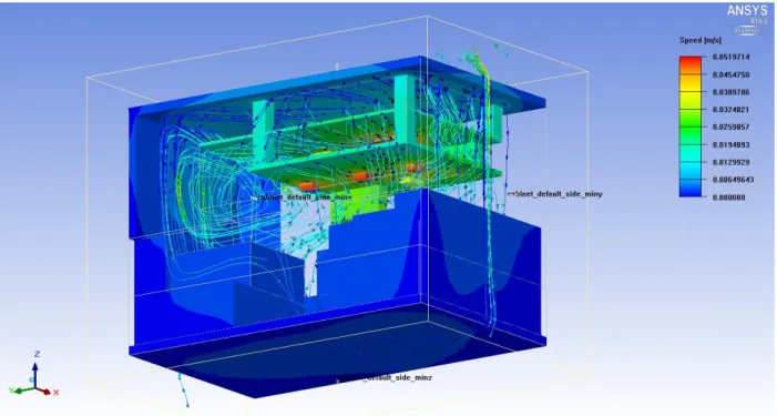
(31) Systems Engineering Power and Control – Bachelor thesis Thermal analysis of a seismic borehole sensor 5.3 Results Here are the results of simulating the existing sensor on Icepak software.. Figure 17 Result of Icepak simulation, housing temperature in open environment. Figure 18 Result of Icepak simulation, air velocity in and out of the housing. Figure 18 and Figure 20 show the plan of the air speed. The velocity of V=0,078 m/s is so small that it doesn’t need to be taken into consideration. This is free air convection.. Jena, 04 September 2015. 27/61. Yves Ravedoni.

(32) Systems Engineering Power and Control – Bachelor thesis Thermal analysis of a seismic borehole sensor. Figure 19 Result of Icepak simulation, components temperatures. Figure 20 Result of Icepak simulation, PCB without housing, air velocity. Jena, 04 September 2015. 28/61. Yves Ravedoni.

(33) Systems Engineering Power and Control – Bachelor thesis Thermal analysis of a seismic borehole sensor. Figure 21 Result of Icepak simulation, PCB without housing, components temperature. The next table presents the power dissipation of each component and the result of the temperatures obtained. In chapter III.1.4 Power dissipation has approximate values. In Table 12 these values have been adapted. Adaptation is made to bring temperatures close to reality (comparison in chapter III.6).. General Heat Sources. Power Dissipation [W]. Ambient OPamp X OPamp Y OPamp Z AD conv. DC/DC conv. Geoph. X Geoph. Y Geoph. Z Processor Usb processor LDO. 0,199 0,199 0,199 0,137 0,2307 0,005 0,005 0,005 0,6486 0,2993 0,135. Icepak sim PCB outside housing [°C] 25 61,9 61,7 63 53,7 45,1 58,6 46,6 54,5. Average values Icepak Delta T sim (with PCB ambient) inside housing [°C] [°C] 25 36,9 69,4 36,7 68,9 38 70,7 28,7 61 20,1 52,9 29,5 29,5 29,5 33,6 69,5 21,6 58,1 29,5 62. Delta T (with ambient) [°C] 44,4 43,9 45,7 36 27,9 4,5 4,5 4,5 44,5 33,1 37. Table 12 Power dissipation of components, and obtained temperature results on Icepak simulation. Jena, 04 September 2015. 29/61. Yves Ravedoni.

(34) Systems Engineering Power and Control – Bachelor thesis Thermal analysis of a seismic borehole sensor 6. Comparison between thermal measurements and simulation results Now simulation results are compared with the reality using the “Delta T” value from Table 8 (page 20) and Table 12.. PCB outside housing. OPamp X OPamp Y OPamp Z AD conv. DC/DC conv. Geoph. X Geoph. Y Geoph. Z Processor Usb processor LDO. Delta T (with ambient) Infrared Icepak Camera simulation VarioCAM Obj. 1.0/30 [°C] [°C]. Absolute Error. Relative Error. [°C]. [%]. 36,9 36,7 38 28,7 20,1 33,6. 30,7 31,8 31,9 28,8 21,9 34,3. 6,2 4,9 6,1 -0,1 -1,8 -0,7. 20% 15% 19% 0% 8% 2%. 21,6 29,5. 19,6 31,5. 2 -2. 10% 6%. Table 13 Comparison between simulation and real temperatures. PCB outside housing. PCB inside housing. OPamp X OPamp Y OPamp Z AD conv. DC/DC conv. Geoph. X Geoph. Y Geoph. Z Processor Usb processor LDO. Delta T (with ambient) Infrared Icepak Camera Absolute simulation VarioCAM Error Obj. 1.0/30 [°C] [°C] [°C]. Relative Error [%]. 44,4 43,9 45,7 36 27,9 4,5 4,5 4,5 44,5. 43,9 46,8 47,3 41,5 37,5 4,5 4,5 4,5 38,6. 0,5 -2,9 -1,6 -5,5 -9,6 0 0 0 5,9. 1% 6% 3% 13% 26% 0% 0% 0% 15%. 33,1 37. -. -. -. Table 14 Comparison between simulation and real temperatures. PCB inside housing. Jena, 04 September 2015. 30/61. Yves Ravedoni.

(35) Systems Engineering Power and Control – Bachelor thesis Thermal analysis of a seismic borehole sensor To get simulation values as close as possible to reality, iterative method has been used. This provides the best results and the least errors. Power dissipation and thermal conductivity of PCB are approximated values that have been adjusted to give the best results.. 6.1 Improvements To improve thermal dissipation of a component, the aim is to reduce the thermal resistance around it. This will keep the component temperature close to the environment temperature (small “Delta T (with ambient)” value). To explain this, let’s make a comparison of Figure 5 (page 10 of chapter III.1.4) and Figure 23. In Figure 23 the thermal resistance is reduced with a “graphite heat spreader” all around the electronic heat source. This conduction resistance (Rgr_cond, graphite heat spreader) will remove the convection and radiation resistance of the heat source component and the inside housing. Graphite heat spreader has a very high thermal conductivity of 100-500 [W *mm-1*K-1]. It will make a good dissipation of the heat from the electric component. The “Delta T (with ambient)” will be smaller.. Figure 22 Three pieces of graphite heat spreaders. Jena, 04 September 2015. 31/61. Yves Ravedoni.

(36) Systems Engineering Power and Control – Bachelor thesis Thermal analysis of a seismic borehole sensor θout. θin. Pd. Rh. Rho_rad. Pd Rb. Rgr_cond. Rho_conv θout. θin Conductivity. Conductivity. Electronic componant. Graphit thermal paste. Conductivity. Outside Radiation + Convection. Housing wall. Figure 23 Thermal flow from an electronic heating source through graphite heat spreader and a housing to environment. In conclusion, to optimise the thermal flow on the existing sensor, thermal graphite heat spreader can be used. The housing should be of steel material with an outside non-metallic lacquer surface. This will reduce thermal resistivity, improve radiation and reduce the “Delta T (with ambient)” of the electronic components.. Jena, 04 September 2015. 32/61. Yves Ravedoni.

(37) Systems Engineering Power and Control – Bachelor thesis Thermal analysis of a seismic borehole sensor. IV.. REALIZATION The existing sensor of chapter III was tested to verify that the simulation results give realistic and reliable values within an acceptable limit of precision. A new sensor is analysed and then simulated to prevent any temperature damage of the sensor while working in high temperatures.. 1. Objectives and criteria The new seismic sensor is designed to make measurements in boreholes. These are static measurements; the sensor is inserted at the bottom of the borehole and may be left there for many years. The borehole seismic measurements provide precise values (the signal to noise ratio will be higher) and quicker seismic results than sensors on earth’s surface. This is because with depth there is an increase in density and more rock. This provides better signal.. 1.1 Environment and conditions The following diagram represents the configuration of the sensor. It can be placed at depths ranging from 200 [m] to 1 [km]. The sensor will be placed at the bottom of the borehole. A 4x 1.5 [mm2] shield cable is used to support the weight of the sensor on extraction. At ground level a PC or a data server presents the measurements. There is also a power supply unit used to administer the sensor in electricity. There are different sizes of borehole. The smallest have a diameter of 90 [mm]. The sensor is designed to have a diameter smaller than 90 [mm].. Jena, 04 September 2015. 33/61. Yves Ravedoni.

(38) Systems Engineering Power and Control – Bachelor thesis Thermal analysis of a seismic borehole sensor. PC + Database. Wave velocity [km/s] 6. 9. 12 Upper mantle. 0.2 - 1 km max 3 km. P-wave S-wave. 15 Depth 0 km. 3. 1 km. 0. 2 km. Sensor. Lower mantle. Seismic waves. Outer core (liquid). ≥ 9cm. 3 km. «D» layer. Figure 24 Representation of the sensor in the earth5. On the right of Figure 24 is the representation of the velocity of earthquake signal. The P-wave is the first signal and the S-wave is the second signal following the P-wave. The graph shows that the velocity of seismic waves increase with depth.. 5. Velocity graph inspired by data from web site “what on Earth” HTTP://WHATONEARTH.OLEHNIELSEN.DK/IMG/SEISMIC_VEL_EARTH.JPG 31.07.15 Jena, 04 September 2015. 34/61. Yves Ravedoni.

(39) Systems Engineering Power and Control – Bachelor thesis Thermal analysis of a seismic borehole sensor 1.2 Mechanical design The mechanical design of the new seismic sensor has been made in the Hes-so. It is designed for the most extreme case. The housing can resist 120 [bar] pressure (24 [bar] nominal, with a 5x security factor). It is made of stainless steel. The outside diameter is 60.32 [mm] for a length of 715 [mm] (variable). Inside there are three geophones, one for every axis, and the PCB. The internal diameter for the PCB is 42.8 [mm]. The length is variable, dependant on the space needed for electronic components.. 60.32. 715. 42.8. 130. 150. Adjustable. Figure 25 borehole sensor, with size in mm 6. For thermal flow simulations, the sensor is simplified as in Figure 26.. 6. Image from „Sismomètre Plan B – A0100“ Christian Cachelin, 25.05.2015, Hes-so Valais-Wallis. Jena, 04 September 2015. 35/61. Yves Ravedoni.

(40) Systems Engineering Power and Control – Bachelor thesis Thermal analysis of a seismic borehole sensor. Figure 26 borehole sensor, made with simplified housing. 1.3 Temperature conditions The sensor is analyzed in two different situations. The two results are studied. The first variant (in chapter IV.2) has the following specifications: an environment temperature Tnominal = 150 [°C] and a maximal environment temperature of T max=180 [°C]. The maximal depth at which it can be placed is 3 [km] long. The second variant (in chapter IV.3) has an environment temperature Tnominal = 70 [°C] and a maximal environment temperature of Tmax=100 [°C]. The maximal depth is 1km long.. Variant 1 : Variant 2 :. Depth. Temp. Max, temp. Pressure. 1-3 km 0.2-1 km. 150 °C 70 °C. 180°C 100 °C. 24 bar 24 bar. Figure 27 General conditions for variant one and two. 1.4 Electronic conception For the 1st variant, compatible components are chosen, which will give good performance at the specified temperatures. In the 2nd variant, the components are given. The power dissipation is set as 9 [W] and comparison is made between a normal design, a design with graphite heat spreader (to improve thermal conductivity) and a design with a Peltier element.. Jena, 04 September 2015. 36/61. Yves Ravedoni.

(41) Systems Engineering Power and Control – Bachelor thesis Thermal analysis of a seismic borehole sensor 1.5 Electrical diagram and components The electronic diagram of the sensor is almost the same as the existing sensor. There are also geophones, operational amplifiers, analogic/digital converters, and a processor. Instead of the wireless device, there is a transmitter that sends data to the computer. Also the power supply must be adapted to suit this borehole sensor.. Power Supply Oscillator. LDO. Converter. DC DC. DC A. X. Computer Device. Y. Z Geophones. D. Operational Amplifiers. Analog/ Digitial Converter. Processor. Transmitter. Figure 28 Borehole sensor, electronic diagram. Jena, 04 September 2015. 37/61. Yves Ravedoni.

(42) Systems Engineering Power and Control – Bachelor thesis Thermal analysis of a seismic borehole sensor 2. Variant 1 The first analysed solution is a sensor running in an average temperature of T= 150 [°C] and a maximal temperature of 180 [°C]. This harsh environment requires high relativity components. The strategy of this variant is to work with electronic components from the category “space”, “avionics” and “drilling holes”. These components are generally built to work to a maximal temperature of 180 [°C], or 210 [°C] with a ceramic housing.. 2.1 Electronic components There are not many components for the category “space”, “avionics” and “drilling holes”. The following components were chose for their compatibility and their general performances. The performance may be improved using other components, but in this case, the red components have been chosen for the simulation. Their Datasheets can be found in annexes 8-18.. Component name. Type. Geophones Operational amplifiers. Analogue/digital converter Processor DC/DC converters Reference Transmittor (RS485). OMNI 2400 SMC 1850 AD8634 AD8229 INA129-HT ADS1282-HT SM470R1B1MHT HTA200 05DN HTB200 03R3SN REF5025-HT SN65HVD. Maximal temperature Datasheet Maximal SOIC Ceramic Power package package Dissipation [°C] [°C] [W] 200 200 175 210 175 210 0.056 175 210 175. 210. -. 150. 220. -. 210 210. 0.165. 185 185 125 175. Table 15 Operating temperatures and power dissipation of components. 2.2 Mechanical design The PCB are set in a triangle in the sensor housing. This solution provides a bigger surface of PCB for the attributed length. It also has the advantage that some flexible PCB parts exist and therefore the three PCBs can be joined as one with two flexible parts.. Jena, 04 September 2015. 38/61. Yves Ravedoni.

(43) Systems Engineering Power and Control – Bachelor thesis Thermal analysis of a seismic borehole sensor. Transmittor. 3x OP amplifier Processor. 2x Reference A/D converter. Figure 29 Variant 1, component disposition on the PCB. The power supplies are voluminous, so they are set individually on a base. The base helps to dissipate the heat to the sensor’s housing.. DC/DC converter 3.3V 5W. DC/DC converter +/- 5V 20W. Figure 30 Variant 1 with two DC-DC converter on a stainless-steel base. Jena, 04 September 2015. 39/61. Yves Ravedoni.

(44) Systems Engineering Power and Control – Bachelor thesis Thermal analysis of a seismic borehole sensor 2.3 Specifications of simulation The flow simulation software “Icepak” is used to analyse the sensor. The round housing has been simplified. The Icepak simulation has these general characteristics: . Gravity vector is in the direction of Z axis. . Air has a laminar flow regime. . Pressure is of 1.01325 bar. . Radiation is activated, all objects have a “radiation to all objects” characteristic. Table 16 shows the attributed solid and surface materials of each component. It may not be the exact name. The chosen materials have emissivity and conductivity values that are close to the real components.. Objects. Surface Material. Housing DC-DC converter General heat sources (components) PCB PCB connexion part. Name Steel-polished casting Steel-Oxidised-surface. Emissivity 0,52 0,8. Ceramic-surface Plastics-infrared Opaque Plastics-infrared Opaque. Solid material Conductivi ty [W*mName 1*K-1] Steel-stainless-300 14,6 Ceramic_material 15,0. 0,9. Ceramic_material. 15,0. 0,9. PCB_solid_material. 5,0. 0,9. PCB_solid_material. 5,0. Table 16 Surface and solid material specification for Icepak simulation variant 1. Jena, 04 September 2015. 40/61. Yves Ravedoni.

(45) Systems Engineering Power and Control – Bachelor thesis Thermal analysis of a seismic borehole sensor 2.4 Results Here are the results of simulating the variant 1 sensor using Icepak software.. Figure 31 Simulation of variant 1, Tamb=180 [°C], housing. Figure 32 Simulation of variant 1, Tamb=180 [°C], inside housing. Jena, 04 September 2015. 41/61. Yves Ravedoni.

(46) Systems Engineering Power and Control – Bachelor thesis Thermal analysis of a seismic borehole sensor. Figure 33 Simulation of variant 1, Tamb=180 [°C], PCB and DC-DC with base. Table 17 presents the attributed power dissipation (the unknown values were approximated). Two environment temperatures have been simulated, the first with T=150 [°C], the second with T=180 [°C] which is the maximal accepted temperature.. Average values General Heating Sources. Type Ambient Geophones OPamp AD conv. Processor DC/DC conv. DC/DC conv. Reference Transmittor. SMC 1850 AD8229 ADS1282-HT SM470R1B1M-HT HTA200 05DN HTB200 03R3SN REF5025-HT SN65HVD. Total power dissipation : Minumum Maximum. Power Dissipation. Simulation One. Simulation Two. [W]. [°C] 150 151 155.3 154.9 166.8 153.6 153.6 154.5 157.5. [°C] 180 181 186.6 186.5 199.7 184.2 184.2 185.8 188.9. 150 166.78. 180 199.7. 0.09 0.056 1 2 1.2 0.035 0.165 4.838. Table 17 Variant 1, components Pd, and simulation temperature values. Jena, 04 September 2015. 42/61. Yves Ravedoni.

(47) Systems Engineering Power and Control – Bachelor thesis Thermal analysis of a seismic borehole sensor The results of simulation show that electronic components can work at the given temperature conditions but they must have a ceramic package (maximal value above 175 [°C]). The geophones will not be submitted to temperatures over 200 [°C], because the temperature of the housing containing the geophones is about 182 [°C]. The DC/DC converters have a limit of 185 [°C]. In the second simulation, they reach 184.2 [°C]. This value is only with maximal environment temperature, so that means that these components will rarely be exposed to temperatures as high as 184.2 [°C]. The results can be improved with a graphite heat spreader all around the converters. That would probably keep converters under 182 [°C].. 2.5 Cost and improvements On variant 1, the cost of the studied electronic components (including geophones) is approximately 2’526 €. On the existing sensor these components have a cost of 659 €. This means that using high temperature components would cost a minimum of four times more than normal components. Because high temperature components are expensive, their need has to be proven. In this case, high temperature components are the best option. The cooling system with a Peltier element is useless, because the environment temperature is too high (the Peltier functionality is explained further in chapter IV.3.2 page 44). An improvement can be made by using graphite heat spreader around the three PCB (see chapter IV.3.6 page 51 for example) and around the two DC/DC converters. As described in chapter III.6.1 (page 31) this will improve thermal conductivity and reduce the temperature of the components.. 3. Variant 2 The second analysed solution is a sensor running in an average temperature of T= 70 [°C] and a maximal temperature of 100 [°C]. In this variant, the components are given. The power dissipation is set as 9 [W]. Comparison will be made between a normal simulation, a simulation with graphite heat spreader and a simulation with a Peltier element.. 3.1 Electronic components All the given components have a maximal temperature of 125 [°C]. Their power dissipation value has no importance because the total power dissipation is set as 9 [W]. The 9 [W] of power dissipation are divided between the PCB’s components as shown in Table 18.. Jena, 04 September 2015. 43/61. Yves Ravedoni.

(48) Systems Engineering Power and Control – Bachelor thesis Thermal analysis of a seismic borehole sensor. General Heating Sources. Quantity. Operational amplifier (OPamp.) Analog/digital converter (AD conv.) Processor Power supply (PS) Reference Transmitter. Power Dissipation. 3. [W] 0,7. 1 1 3 2 1. 1 1,6 1 0,5 0,3. Total power dissipation. 9. Table 18 Components and their power dissipation for variant 2. 3.2 Peltier element The Peltier element is a static component creating a heat flux between two surfaces. It is also called a TEC (thermoelectric cooler). This component is used in many applications (for example: car fridge). It is cheap but it has a bad efficiency. As represented in Figure 34, a current is passes through a semiconductor that creates a temperature difference at each end (Peltier effect). Placed in parallel, semiconductors present two surfaces with different temperatures. A flow is created from the cold to the hot side. The maximal difference between the two surfaces is 70 [°C].. Figure 34 Design of Peltier element, with description 7. Equation 7 shows that the amount of heat on the hot side is equal to the sum of the electric power consumption and the amount of heat on the cold side.. 𝑄ℎ = 𝑃𝑒𝑙 + 𝑄𝑐 [W] Equation 7. 7. Figure from : http://home.arcor.de/glaube.u/spf-modul/Construction%20of%20TEM%20N.html. Jena, 04 September 2015. 44/61. Yves Ravedoni.

(49) Systems Engineering Power and Control – Bachelor thesis Thermal analysis of a seismic borehole sensor The electric power consumption depends on the amount of heat to evacuate (cold side) and the difference of temperature needed. A Peltier element has not been chosen, because of wrong results of simulation.. 3.3 Mechanical design The PCB are still set in a triangle. This has a length of 150mm instead of 120mm (Variant 1) because the power supplies are included on the PCB and not on a separate base.. 3x Power supply. Transmittor 3x OP amplifier Processor. 2x Reference. A/D converter Figure 35 Variant 2, component disposition on the PCB. Figure 36 shows the housing for the Peltier element simulation. This is an experimentation to analyse if a thermos design built with two Peltier element would provide better performance. For this design, the diameter of the sensor had to be expended to an outside diameter of D=88mm. The inner thermos diameter is the same as in variant 1.. Jena, 04 September 2015. 45/61. Yves Ravedoni.

(50) Systems Engineering Power and Control – Bachelor thesis Thermal analysis of a seismic borehole sensor. Figure 36 Housing designed with Peltier and thermos. Two Peltier elements have been placed, one at each end of the inner tube. The cold sides are placed on the inner tube, the hot sides are place on the housing to dissipate the heat to the environment.. 3.4 Specifications of simulation The flow simulation software “Icepak” is used to analyse the sensor. The round housing has been simplified. The Icepak simulation has these general characteristics: . Gravity vector is in the direction of Z axis. . Air has a laminar flow regime. . Pressure is of 1.01325 bar. . Radiation is activated, all objects have a “radiation to all objects” characteristic. Table 19 shows the attributed solid and surface materials of each component. It may not be the exact name. The chosen materials have emissivity and conductivity values that are close to the real components.. Jena, 04 September 2015. 46/61. Yves Ravedoni.

(51) Systems Engineering Power and Control – Bachelor thesis Thermal analysis of a seismic borehole sensor Objects. Surface Material Name. Housing General heat sources (components) PCB PCB connexion part Graphite heat spreader. Emissivity. Steel-polished casting. 0,52. Ceramic-surface Plastics-infrared Opaque Plastics-infrared Opaque. 0,9 0,9 0,9. Plastics-infrared Opaque. 0,9. Solid material Conductivi Name ty [W*m1*K-1] Steel-stainless-300 14,6 Ceramic_material PCB_solid_material PCB_solid_material eGRAF_HITHERM_ SRS_700. 15,0 5,0 5,0 240,0. Table 19 Surface and solid material specification for Icepak simulation variant 2. 3.5 Results Figure 37 and Figure 38 are the “simulation 1” with the normal housing without graphite.. Figure 37 Simulation 1 of variant 2, Tamb = 100 [°C], without graphite, housing. Jena, 04 September 2015. 47/61. Yves Ravedoni.

(52) Systems Engineering Power and Control – Bachelor thesis Thermal analysis of a seismic borehole sensor. Figure 38 Simulation 1 of variant 2, Tamb = 100 [°C], with graphite, PCB. Figure 39 and Figure 40 are the “simulation 2” with graphite heat spreader all around the PCB.. Figure 39 Simulation 2 of variant 2, Tamb = 100 [°C], with graphite heat spreader (not represented). Jena, 04 September 2015. 48/61. Yves Ravedoni.

(53) Systems Engineering Power and Control – Bachelor thesis Thermal analysis of a seismic borehole sensor. Figure 40 Simulation 2 of variant 2, Tamb = 100 [°C], graphite heat spreader and PCB. Figure 41 and Figure 42 are the “simulation 3” with two Peltier elements. Each Peltier element is set to absorb Qc = 7 [W] (half of 9 [W] with a safety margin).. Figure 41 Simulation 3 of variant 2, Tamb = 100 [°C], with Peltier elements, inside thermos tube. Jena, 04 September 2015. 49/61. Yves Ravedoni.

(54) Systems Engineering Power and Control – Bachelor thesis Thermal analysis of a seismic borehole sensor. Figure 42 Simulation 3 of variant 2, Tamb = 100 [°C], with Peltier elements, PCB. The Peltier elements were simulated only with the absorbing Qc value. Unfortunately no realistic solutions were found when the dispersion value Qh was set. This means approximately 14 [W] were extracted from the inner thermos, but no heat flow was transferred to the outside housing. This simulation result of Peltier elements is therefore the “best case possible”. Two environment temperature have been simulated, the first with T=70 [°C], the second with T=100 [°C] which is the maximal accepted temperature.. General Heating Sources. Simulation 1 Normal Housing. Simulation 2 with graphite H. spreader. Simulation 3 With Peltier. [W]. [°C] 70. [°C] 70. [°C] 70. 0,7 1 1,6 1 0,5 0,3. 128,1 123,3 140,5 128,6 131,8 123,6. 90,7 89,7 90,4 90,2 93,1 90,4. 102,2 93,3 112,4 99,3 102,6 92,9. 70 140,6. 70 95. 58,3 112,4. Power Dissipation. Ambiant OPamp. AD conv. Processor P. supply Reference Transmitter Minimum Maximum. Table 20 Variant 2, Tamb = 70 [°C], components Pd, and simulation temperature values. Jena, 04 September 2015. 50/61. Yves Ravedoni.

(55) Systems Engineering Power and Control – Bachelor thesis Thermal analysis of a seismic borehole sensor. General Heating Sources. Simulation 1 Power Normal Dissipation Housing [W]. [°C] 100. [°C] 100. [°C] 100. 0,7 1 1,6 1 0,5 0,3. 151,1 148,1 164,7 153,8 156,2 148,1. 118,1 117,2 117,9 117,5 120,2 117,8. 122,8 129,2. 100 164,7. 100 122,4. 141,2 89,5. Ambiant OPamp. AD conv. Processor P. Supply Reference Transmitter Minimum Maximum. Simulation 2 Simulation 3 with With graphite H. Peltier spreader. 128,9 131,6 141,2. Table 21 Variant 2, Tamb = 100 [°C], components Pd, and simulation temperature values. The simulation 1 with the normal housing demonstrates that this design is not good because all components are above 125 [°C] (the maximal operating temperature of components). This case even with an ambient temperature of Tamb = 70 [°C]. The simulation 2 with the graphite heat spreader gives reliable results. The results of simulation 3 with the Peltier element are not very satisfactory. At T amb = 100 [°C], the processor and the transmitter heat over 125 [°C]. Even if results are “best case possible”, they are not as good as the graphite heat spreader.. 3.6 Improvements The Simulation 3 with Peltier element has no convincing results. Figure 43 shows that at an ambient temperature of 100 [°C], components will be over 125 [°C]. In comparison with simulation 1, improvements are not significant (20 [°C] less). The mechanical design is more complex, therefore more expensive. The electrical consumption of Peltier element is not negligible (about 10-20 [W] per TEC) and the obtained results are not guaranteed. The Simulation 2 with the graphite heat spreader is the best of these solutions. Further improvements could possibly be achieved using less graphite. The graphite doesn’t need to be on all the length of the PCB; it could be limited to the area around the components. Graphite heat spreader is not expensive, it is easy to add to the design. Care must be taken for electrical insulation between the PCB and the graphite.. Jena, 04 September 2015. 51/61. Yves Ravedoni.

(56) Systems Engineering Power and Control – Bachelor thesis Thermal analysis of a seismic borehole sensor. Comparison of temperatures between simulations of variant 2 175 Sim1 - Normal housing 100 [°C]. Temperature [°C]. 150. Sim 2 - With graphite H. S. 100 [°C] Sim 3 - With Peltier 100 [°C]. 125. Sim 1 - Normal housing 70 [°C]. 100. Sim 2 - With graphite H. S. 70 [°C] Sim 3 - With Peltier 70 [°C]. 75. Limite Max 125 [°C] Composants Figure 43 Comparison of the temperatures between simulations of variant 2. A design with Peltier element and graphite heat spreader in a thermos would probably be the best solution.. Jena, 04 September 2015. 52/61. Yves Ravedoni.

(57) Systems Engineering Power and Control – Bachelor thesis Thermal analysis of a seismic borehole sensor 4. Analysis Comparison between the existing sensor, variant 1 and variant 2.. 4.1 Performance of models Regarding the temperature, three models have been studied. The following table shows each design adapted to an appropriate temperature.. Ambient temperature. 25 [°C] - [°C] max. Adapted model. Existing sensor. Maximal component value Pressure Cost of studied electronic components. 70,7 (@25[°C]) - [bar] 659 €. 70 [°C] 100 [°C] max Variant 2 With graphite heat spreader 93,1 (@70[°C]) 120,2 (@100[°C]) 25 [bar] 1’150 €. 150 [°C] 180 [°C] max Variant 1 With high temperature components 166,8 (@150[°C]) 199,9 (@180[°C]) 25 [bar] 2’550 €. Figure 44 Adapted model for a specific ambient temperature. The two variants have a maximal “delta T with ambient” value of 20 [°C]. The existing sensor has a maximal “delta T with ambient” value of 45,7 [°C]. This is because during the development of the existing sensor, no interest has been taken to thermal flow. All models have a different number of components, a different total power dissipation value and a different ambient temperature therefore it is difficult to make a general thermal analysis. Every model is analysed in its specific “Improvement” chapter.. 4.2 Cost The existing sensor with its components has a cost of 659 €. In variant 1, the cost of the studied electronic components (including geophones) is approximately 2’550 €. In variant 2, the cost of electronic components (including geophones) is approximately 1’150 €. The existing sensor is not expensive, but it is not ready to be sold, some improvements should first be made. This could require more components, and may increase the price. The variant 1, with high temperature components would cost a minimum of four times more than normal components. This is the cost of components from the category “space”, “avionics” and “drilling holes”. The advantage of this conception is that it is able to work at 180 [°C]. The variant 2, with components from the category “automotive”, would cost a minimum of 1’150€. The new housing has no attributed price.. Jena, 04 September 2015. 53/61. Yves Ravedoni.

(58) Systems Engineering Power and Control – Bachelor thesis Thermal analysis of a seismic borehole sensor 4.3 Improvements At this time, the conception requires to be built. Then thermal measurements should be made at operating temperatures. The measurement results would certify simulations and give advice for future improvements. Then, at this point, further simulation of the sensor could be made. According to mechanical possibilities of designs further PCB disposition in the housing could also be simulated. Such as two vertical PCBs in parallel, or “x” horizontal PCBs in parallel. The Peltier element should be more studied to have correct simulation results. Then other designs with Peltier element could be simulated to found the best and cheapest result. For example the Peltier element could be set on the electronic components.. Jena, 04 September 2015. 54/61. Yves Ravedoni.