HAL Id: hal-01133693
https://hal.archives-ouvertes.fr/hal-01133693
Submitted on 20 Mar 2015HAL is a multi-disciplinary open access
archive for the deposit and dissemination of sci-entific research documents, whether they are pub-lished or not. The documents may come from teaching and research institutions in France or
L’archive ouverte pluridisciplinaire HAL, est destinée au dépôt et à la diffusion de documents scientifiques de niveau recherche, publiés ou non, émanant des établissements d’enseignement et de recherche français ou étrangers, des laboratoires
New bounds for the inhomogenous Burgers and the
Kuramoto-Sivashinsky equations
Michael Goldman, Marc Josien, Felix Otto
To cite this version:
Michael Goldman, Marc Josien, Felix Otto. New bounds for the inhomogenous Burgers and the Kuramoto-Sivashinsky equations. Communications in Partial Differential Equations, Taylor & Francis, 2015. �hal-01133693�
New bounds for the inhomogenous Burgers and
the Kuramoto-Sivashinsky equations
Michael Goldman
∗, Marc Josien
†and Felix Otto
‡March 19, 2015
Abstract
We give a substantially simplified proof of the near-optimal estimate on the Kuramoto-Sivashinsky equation from [14], at the same time slightly improving the result. The result in [14] relied on two ingredients: a regularity estimate for capillary Burgers and an a novel priori estimate for the inhomogeneous inviscid Burgers equation, which works out that in many ways the conservative transport nonlinearity acts as a coercive term. It is the proof of the second ingredient that we substantially simplify by proving a modified Kármán-Howarth-Monin iden-tity for solutions of the inhomogeneous inviscid Burgers equation. We show that this provides a new interpretation of the results obtained in [7].
1 Introduction
1.1 The Kuramoto-Sivashinsky equation
We consider the one-dimensional Kuramoto-Sivashinsky equation:
∂tu + u∂xu + ∂2xu + ∂4xu = 0. (K-S)
This equation appears in many physical contexts, in particular in the modeling of surface evolutions. Sivashinsky used it to describe flame fronts [16], wavy flow of vis-cous liquids on inclined planes [17] and crystal growth [6]. Although the solutions
∗LJLL, Université Paris Diderot, CNRS, UMR 7598, France, email:
goldman@math.univ-paris-diderot.fr
†Ecole Polytechnique, Palaiseau, France, email: marc.josien@polytechnique.edu
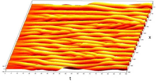
of (K-S) are smooth and even analytic [10], they display a chaotic behavior for suffi-ciently large systems size L (see [9] and Figure 1.1). The structure of the Kuramoto-Sivashinsky equation has some similarities with the Navier-Stokes equation. There-fore, it is sometimes possible to apply similar techniques to study both equations (see [15]).
Figure 1: Chaotic behavior of u
For a given system size L > 0, we will consider L-periodic solutions of (K-S). Since the spatial averageRL
0 u(t , x)d x is constant over time, and since the equation is
in-variant under the Galilean transformation:
t = t0, x = x0+U t , u = u0+U , it is not restrictive to assume thatR0Lu(t , x)d x = 0 for all t ≥ 0.
We can artificially cut the equation in two parts and consider separately the two mechanisms involved in (K-S):
∂tu + ∂2xu + ∂4xu = 0, (1)
∂tu + u∂xu = 0. (2)
The first equation (1) is linear and can be seen in Fourier space as:
The fourth partial derivative term∂4xu decreases the short wavelength part of the
en-ergy spectrum whereas the second derivative term∂2xu amplifies the long wavelength
part. The second equation (2) corresponds to Burgers equation. It is nonlinear and develops shocks in finite time for non-trivial initial data. Nevertheless, as we will see later, this term has some mild regularizing effect. It is worth mentioning that for (2), the energy
Z L
0
u2d x,
is conserved. Therefore, one can intuitively say that in (K-S) the linear terms trans-port the energy from long wavelengths to short ones. Numerical simulations suggest (see the article of Wittenberg and Holmes [19]) that the time-averaged power spec-trum lim T →∞(LT ) −1 Z T 0 |F (u)(t,ξ)| 2 d t
is independent of L for L À 1. Moreover, this quantity is independent of |ξ| and L À 1 in the long wavelength regime L−1¿ |ξ| ¿ 1 and decays exponentially in the short wavelength regime |ξ| À 1. In line with this, numerical simulation suggests that for allα ≥ 0: lim sup T →∞ (LT )−1 Z T 0 Z L 0 ¡|∂x| αu¢2 d xd t = O(1).
This conjecture is supported by a universal bound on all stationary periodic solutions of (K-S) with mean 0, due to Michelson [12].
1.2 Known bounds
A first energy bound was obtained in the 80’s by Nicolaenko, Scheurer and Temam [13], who established by the “background flow method” that for every odd (in space) solution u of (K-S): lim sup t →∞ µ 1 L Z L 0 u2d x ¶1/2 = O(Lp),
with p = 2. This has been later generalized by Goodman [8], and Bronski and Gambill [2] and improved to p = 1. Using an entropy method, Giacomelli and the third author [5] improved this result by showing that:
lim sup t →∞ µ 1 L Z L 0 u2d x ¶1/2 = o(L).
The proof is based on the fact that the dispersion relationξ2−ξ4in (3) vanishes for
ξ → 0 and it implies that for every α ∈ [0,2], we have:
lim sup T →∞ µ 1 T L Z T 0 Z L 0 ¡|∂x| αu¢2 d xd t ¶1/2 = o(L),
by using the energy identity, ∂t Z L 0 (u(t , x))2d x = Z L 0 (∂xu(t , x))2d x − Z L 0 ¡ ∂2 xu(t , x)¢ d x.
In a more recent paper [14], the third author proved that, for allα ∈ (1/3,2),
lim sup T →∞ µ 1 T L Z T 0 Z L 0 ¡|∂x| αu¢2 d xd t ¶1/2 = O¡ln5/3+(L)¢ ,1 (4) by using two ingredients: an a priori estimate for the capillary Burgers equation
∂tu + u∂xu + ∂4xu = |∂x|g and an a priori estimate for the inhomogeneous Burgers
equation, that is∂tu + u∂xu = |∂x|g . More precisely, the result of [14] states that, for
every solution u of (K-S),
kukB1/3
3,3 = O¡ln
5/3+(L)¢ , (5)
where k·kBs
p,r denotes a Besov norm (see the appendix).
1.3 Main result
In this paper, we improve and simplify the result of the third author by showing that:
Theorem 1.1. Let L > 2. For u a smooth L-periodic solution with zero average of the
equation ∂tu + u∂xu + ∂2xu + ∂4xu = 0, there holds lim sup T →∞ µ sup h>0 1 LT Z T 0 Z L 0 |u(t , x + h) − u(t , x)|3 h d xd t ¶1/3 = O(ln1/2+(L)). (6)
This result is indeed slightly stronger than the previous one, since by (19), it im-plies an improvement of the exponent in (5) from 5/3+ to 5/6+. However, this is not the main contribution of this paper. It is rather a simplified proof of the a pri-ori estimate for inhomogeneous Burgers equation, which was one of the main tool for proving (5). For this purpose, we derive a modified Kármán-Howarth-Monin for-mula (see (14)). We also show how the proof of Golse and Perthame [7] (based on the kinetic formulation of Burgers equation) of a similar estimate for the homogeneous Burgers equation can be reinterpreted in this light. Since we work with slightly dif-ferent Besov norms compared to [14], we need also to adapt most of the other steps to get (6). Besides Proposition 2.5, which we borrow directly from [14], we give here
1we use the notation O(ln5/3+(L)) to indicate that for everyκ > 5/3, there exists c > 0 such that the
self-contained proofs.
The structure of the paper is the following: In Section 2, we enunciate the main theorem and give the structure of the proof. It has several ingredients: a Besov es-timate for the inhomogeneous inviscid equation (Proposition 2.3), a regularity esti-mate for the capillary Burgers equation (Proposition 2.5) and an inverse estiesti-mate for Besov norms on solutions of (K-S) (Proposition 2.7). The following sections (i.e. Sec-tion 3, 4 and 5) are devoted to the proofs. In the appendix, we recall definiSec-tions and a few classical results regarding Besov spaces.
General notations
We denote by Dh the finite-difference operator Dh : u 7→ u(x + h) − u(x), by Lp the space Lp([0, T ] × [0,L]) and for k ∈ N,L > 0, by CLk=© f ∈ Ck(R), f is L − periodicª.
For an L-periodic function u, the spatial Fourier transform is defined by: F (u)(ξ) = L−1Z L
0 exp(−iξx)u(x)dx
and for a Schwartz functionφ: F (φ)(ξ) =
Z
Rexp(−iξx)φ(x)dx.
For v ∈R, we let v+= max(v, 0) (and similarly, v−= max(−v, 0)).
2 Main theorem and structure of the proof
In this section, we state the main theorem and the results on which it is based (see the appendix for the definition and main properties of Besov spaces).
2.1 Main theorem
Theorem 2.1. Let L > 2. For a smooth L-periodic solution u with zero average of (K-S),
there holds kukB1/3 3,∞+ kukB 2 2,2= O(ln 1/2+(L)). (7)
From this theorem, we derive by interpolation (57) the following corollary:
Corollary 2.2. Let L > 2. For a smooth L-periodic solution u with zero average of (K-S)
and for indices p, s and r related by
we have
kukBs
p,r= O(ln
1/2+(L)).
2.2 Structure of the proof
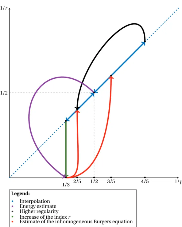
The proof of Theorem 2.1 uses four important ingredients: a regularity result for Burgers equation (Proposition 2.3), a higher regularity estimate for the capillary Burg-ers equation (Proposition 2.5), an energy estimate (Lemma 2.6), and a result which allows us to “increase” the r index of Besov spaces (Proposition 2.7). Let us now sketch the proof, discarding lower-order terms (in particular all the terms contain-ing g = −|∂x|−1∂2xu) and taking borderline exponents in the estimates2. The strategy
is graphically represented in Figure 2. The starting point is Proposition 2.3, which for
s = 1, p = 5/2, r = 5/2 andξ = −|∂x|−1∂4xu (recall also (59)), roughly says that
kuk3B1/3
3,∞.kukB 1
5/2,5/2kukB35/3,5/3.
Using then the interpolation inequality (57), we get kukB3 5/3,5/3.kuk 1/3 B5 5/4,5/4 kuk2/3B2 2,2 .
Proposition 2.5 forα = 2, p = 5/4, q = 5/2 and therefore α0= 1, indicates that kukB5 5/4,5/4.kuk 2 B1 5/2,5/2 . (8)
Using the interpolation inequality (57) once again, we find kukB1 5/2,5/2.kuk 3/5 B1/3 3,3 kuk2/5B2 2,2 . (9)
From Lemma 2.6, we obtain
kukB2
2,2.kukB1/33,∞.
2Let us stress that we cannot reach these exponents since some of the constants (in particular the
Figure 2: Strategy of the proof 1/3 • • 2/5 1/2• 3/5• 4/5• 1/2 • • • • • Legend: • Interpolation • Energy estimate • Higher regularity • Increase of the index r
• Estimate of the inhomogeneous Burgers equation • • • • • • 1/3 • • 2/5 1/2• 3/5• 4/5• 1/r 1/p
At this point, we see that we could have buckled the estimates if in (9), the Besov norm kukB1/3
not doable with our method of proof. Therefore, we need Proposition 2.7 in order to control kukB1/3
3,3 by kukB1/33,∞. It is at this last stage that we lose a logarithm since (19)
gives kukB1/3 3,3 .ln 1/3 (L) kukB1/3 3,∞.
Putting all these estimates together, we find kukB1/3
3,∞.ln
1/2
(L), which is (7).
As mentioned, the first ingredient is an estimate for the inhomogeneous Burgers equation. A similar estimate was obtained in [14, Prop. 1]. A related inequality for the homogeneous Burgers equation has been recently derived in [7].
Let us consider the following inhomogeneous Burgers equation:
∂tu + u∂xu = |∂x| g + |∂x|ξ. (10)
Proposition 2.3 (Besov estimate for the inhomogeneous Burgers equation). Letξ, g
be smooth L-periodic functions. Then, for any smooth L-periodic solution u of (10), there holds: For s ∈]0,1[, r,r0, p, p0∈ [1, +∞] verifying 1r +r10 = 1 and p1+p10 = 1, there
exists a constant c > 0 just depending on s,r, p such that:
kuk3B1/3 3,∞≤c µ kukB1/3 3,∞ ° °g ° ° B3/2,12/3 + kukBp,rs kξkB1−s p0,r 0+ ku(0, ·)k 2 L2[0,L] ¶ . (11)
Therefore, taking the time-space average, it holds:
kuk3B1/3 3,∞≤c µ kukB1/3 3,∞ ° °g ° ° B2/3 3/2,1+ kukB s p,rkξkB1−s p0,r 0 ¶ . (12)
The proof of (11) is based on a modified Kármán-Howarth-Monin identity:
Lemma 2.4. Letη be a smooth L-periodic function and let u be a smooth L−periodic
solution with zero average of
∂tu + u∂xu = η, (13) then for h ∈R, ∂t µ 1 2 Z L 0 |D h u|Dhud x ¶ + ∂h 1 6 Z L 0 |D h u|3d x = Z L 0 Dhη|Dhu|d x. (14) The usual Kármán-Howarth-Monin identity [4] states that
∂t µ 1 2 Z L 0 ³ Dhu´2d x ¶ + ∂h 1 6 Z L 0 ³ Dhu´3d x = Z L 0 DhηDhud x. (15)
This formula can be easily checked by using equation (13) and the periodicity. The main difference between (15) and (14) is that in the latter, the coercive termRL
0 |Dhu|3d x
replaces the non-coercive termR0L¡Dhu¢3
d x.
We will give two proofs of (14). The first is by a direct computation and the second uses the kinetic formulation of Burgers equation following ideas of [7]. Therefore, this second proof gives a new, and hopefully interesting, interpretation of the arguments of [7].
The second ingredient is a higher regularity result for the capillary Burgers equa-tion (see [14, Prop. 2, p. 14]).
Proposition 2.5 (Higher regularity). Let p, q ∈ [1,+∞[, α ∈R satisfying:
p + 1 ≤ q ≤ 2p, and α0= (6 + α)p/q − 3 ∈]0, 1[.
Then, there exists c > 0 such that, if u, g are smooth, L-periodic in x and satisfy ∂tu + u∂xu + ∂4xu = |∂x| g ,
the following estimate holds:
kukB3+α p,p ≤ c µ kukq/p Bα0q,q +°°g ° ° Bαp,p ¶ . (16)
Proposition 2.5 allows to jump from higher derivatives to smaller ones in Besov spaces. The proof, which we will not provide, is based on a narrow-band Littlewood-Paley decomposition.
The third ingredient is an elementary energy estimate, which directly bounds the L2¡[0,T ], H2([0, L])¢∼= B2,22 norm of a solution u of the inhomogeneous capillary
Burgers equation.
Lemma 2.6 (Energy estimate). Let u be a smooth solution of:
∂tu + u∂xu + ∂4xu = |∂x| g . (17)
Then, the following estimate holds:
kukB2 2,2≤ c kuk 1/2 B1/3 3,∞ ° °g ° ° 1/2 B2/3 3/2,1 . (18)
Proof. Since the proof is straightforward, we give it now. Integrating over the
equa-tion (17) over [0, T ] × [0,L], we get: Z L 0 u(T, x)2d x − Z L 0 u(0, x)2d x = Z T 0 Z L 0 u |∂x| g d xd t − Z T 0 Z L 0 (∂2xu)2d xd t . Therefore by (58) Z T 0 Z L 0 ¡ ∂2 xu ¢2 d xd t ≤ Z L 0 u(0, x)2d x + kukB1/3 3,∞ ° °g ° ° B3/2,12/3 ,
As already mentioned, these three estimates will not be sufficient to conclude. We will also need an estimate relating Besov norms with different exponents r . One can easily see that if r1> r2, then k·kBs
p,r1 ≤ k·kBsp,r2 (it is a consequence of convexity inequality). In fact, it is possible to reverse the inequality for solutions of (K-S), but this comes with a price: a logarithm of the spatial period L appears.
Proposition 2.7 (Increasing the index r ). There exists c > 0 such that, for all L ≥ 2, u
solution of (K-S), the following estimate holds:
kukB1/3 3,3 ≤ c ln 1/3 (L) kukB1/3 3,∞. (19)
3 Proof of Theorem 2.1
In this section, we derive the main theorem from the above propositions. We now consider the rescaled Besov normBsp,r as a point (s, 1/p, 1/r ) in the spaceR3. All the norms involved in our problem lie in the rectangleP of R3defined by3:
s = 10/p − 3, 1 p ∈ [0, 1], 1 r ∈ [0, 1].
Proof of Theorem 2.1. Let u be a solution of (K-S). It is convenient to introduce the
abbreviation:
D(α) = kukB10α−3
α−1,α−1 D∗(1/3) = kukB
1/3 3,∞.
Notice that D (1/2) = kukB1/2
2,2 and D (1/3) = kukB1/33,3. With this notation, interpolation
inequality (57) takes the form
D(α) ≤ Dθ(α1)D1−θ(α2) (20)
forα = θα1+ (1 − θ)α2andθ ∈ [0,1].
Letting s = 10α − 3, p = α−1and r = α−1in (12) and using (59) forξ = −|∂x|−1∂4xu,
(12) can be rewritten as
D∗3(1/3) ≤ c³D(α)D(1 − α) + D∗(1/3) kg kB2/3 3/2,1
´
, (21)
forα ∈]3/10,2/5[. In turn, (16) with p−1= β, q−1= γ and α = 10β − 6 (which implies
α0= 10γ − 3) gives D(β) ≤ c µ Dβ/γ(γ) + kgk B10β−1,β−1β−6 ¶ , (22)
forγ ∈]3/10,2/5[ and1−γγ ≤ β ≤ 2γ. Finally, (18) is equivalent to D (1/2) ≤ cD1/2∗ (1/3) kg k1/2B2/3 3/2,1 , (23) and (19) to D (1/3) ≤ c ln1/3(L)D∗(1/3) . (24) Our first goal is to argue that for g = −|∂x|−1∂2xu, we can replace in the above
estimates all the Besov norms involving g by D∗(1/3). By (59) and (57), kg kB10β−6 β−1,β−1 ≤ ckukB10β−5 β−1,β−1 ≤ ckuk1/2 B10β−1,β−1β−3 kuk 1/2 B10β−1,β−1β−7 = cD 1/2(β)kuk1/2 B10β−1,β−1β−7 .
Hence, in view of (23), Young’s inequality and since by (59), kg kB2/3
3/2,1 ≤ ckukB 5/3 3/2,1, it
will be enough to prove that kukB10β−7
β−1,β−1
+ kukB5/3
3/2,1≤ c(D∗(1/3) + D (1/2)) (25)
for β ∈]11/15,4/5[ (which reduces the use of (22) to γ ∈]1/3,2/5[). We can indeed prove more generally that for 1/3 < s < 2, p ≤ 2 and any q ≥ 1, there holds
kukBs p,q≤ c ³ kukB2 2,2+ kukB1/33,∞ ´ . (26)
Thanks to Jensen’s inequality, we have kukBs
p,q ≤ kukBs2,q and kukB1/33,∞ ≥ kukB1/32,∞. By
monotonicity of the Besov norms with respect to the last index, there also holds kukBs
2,q≤ kukB
s
2,1and kukB22,2≥ kukB 2
2,∞. Therefore, we are left with proving that
kukBs 2,1≤ c ³ kukB1/3 2,∞+ kukB 2 2,∞ ´ . By definition of the Besov norms, for 1/3 < s < 2,
kukB2,1s = X k≥0 2kkukkL2+ X k<0 2kkukkL2 ≤ sup k 22kkukkL2 X k≥0 2−k+ sup k 213kku kkL2 X k≤0 223k ≤ c ³ kukB1/3 2,∞+ kukB 2 2,∞ ´ ,
which after taking the average over time and space, finishes the proof of (26). To sum up, we now have that (21), (22) and (23) together with (25) imply
D∗3(1/3) ≤ c¡D(α)D(1 − α) + D2 ∗(1/3)
¢
forα ∈]3/10,2/5[,
D(β) ≤ c³Dβ/γ(γ) + D∗(1/3) ´
(28) forγ ∈]1/3,2/5[ and 1−γγ ≤ β ≤ 2γ and
D (1/2) ≤ cD∗(1/3) . (29)
We now gather the above estimates in order to bound D∗(1/3). Passing to the logarithm in the above inequalities, we see that optimizing the parameters to get the best power of ln(L) is equivalent to a linear programming problem. Its solution thus lie at the boundaries of the admissible domain. It is not hard to see that in particular, we want to take β2 = γ = α with α as close as possible to 2/5. Let θ, η ∈]0, 1[ be such that (1 − α) = θβ + (1 − θ)1 2 and α = η 1 2+ (1 − η) 1 3, so thatθ is close to 1/3 and η is close to 2/5. Thanks to (20),
D(1 − α) ≤ Dθ(β)D1−θ(1/2) and D(α) ≤ Dη(1/2)D1−η(1/3). (30) Since we can assume that D∗(1/3) ≥ 1, we get from (27), (30) and (28),
D∗3(1/3) ≤ cD(α) ³ D2θ(α) + Dθ∗(1/3) ´ D1−θ(1/2) ≤ c ³ D1+2θ(α)D1−θ∗ (1/3) + D(α)D∗(1/3) ´ ,
where in the last inequality, we used (29). From (30), (29) and (24), we deduce
D3∗(1/3) ≤ c ³ D2+θ∗ (1/3) ln13(1+2θ)(1−η)(L) + D2 ∗(1/3) ln 1−η 3 (L) ´ .
Dividing by D∗2(1/3) this inequality and noticing that forη close to 2/5,1−η3 is close to 1/5, we obtain that if D∗(1/3) ≥ ln1−η3 (L), then
D∗(1/3) ≤ cDθ∗(1/3) ln13(1+2θ)(1−η)(L),
which gives finally
D∗(1/3) ≤ c ln13
(1+2θ)(1−η) 1−θ (L)
4 Proof of Proposition 2.3
For the reader’s convenience, let us recall the statement of Proposition 2.3. Let u be a smooth solution of the following inhomogeneous Burgers equation:
∂tu + u∂xu = |∂x| g + |∂x|ξ. (31)
Proposition. Letξ, g be smooth L-periodic functions. Then, for any smooth L-periodic
solution u of (31), there holds: For s ∈]0,1[, r,r0, p, p0∈ [1, +∞] verifying 1r +r10= 1 and
1
p+
1
p0= 1, there exists a constant c ∈R∗+just depending on s, r, p such that:
kuk3B1/3 3,∞ ≤c µ kukB1/3 3,∞ ° °g ° ° B3/2,12/3 + kukBp,rs kξkBp0,r 01−s + ku(0, ·)k 2 L2[0,L] ¶ .
Before proceeding further, let us remark that, by approximation, this applies to any (possibly non smooth) entropy solution of Burgers equation (31). Indeed, if we consider a solution u of
∂tu − u∂xu − ε∂2xu = 0,
then it is a smooth solution of (31) with g = 0 and ξ = ε|∂x| u. A careful inspection of
the proof of Proposition 2.3 shows that for p = r = 2 it extends to s = 1, yielding kuk3B1/3 3,∞≤ c ³ kukB1 2,2kξkB 0 2,2+ ku(0, ·)k 2 L2[0,L] ´ , that is kuk3B1/3 3,∞ ≤ c³εk∂xuk2L2+ ku(0, ·)k2L2[0,L] ´ .
Combining this with the energy inequality:εk∂xuk2L2≤ c ku(0, ·)k2L2[0,L], gives
kuk3B1/3
3,∞≤ c ku(0, ·)k
2
L2[0,L],
which passes to the limit asε → 0. The indices are optimal in the light of the result of De Lellis and Westdickenberg [3] which states that we cannot hope to have more regularity, in the sense that the Besov index s cannot be better than 1/3.
As already pointed out, the proof of the aimed estimate is based on a modified Kármán-Howarth-Monin identity:
Lemma 4.1. Letη be a smooth L-periodic function and let u be a smooth L−periodic
solution with zero average of
∂tu + u∂xu = η (32) then for h ∈R, ∂t µ 1 2 Z L 0 |D h u|Dhud x ¶ + ∂h 1 6 Z L 0 ¯ ¯ ¯D hu¯¯ ¯ 3 d x = Z L 0 Dhη ¯ ¯ ¯D hu¯¯ ¯ d x . (33)
Proof. By periodicity, (33) will be a direct consequence of the following pointwise identity: 1 2∂t ³ |Dhu|Dhu´+1 6∂h ¯ ¯ ¯D hu¯¯ ¯ 3 +1 2∂x µ u|Dhu|Dhu +1 3|D h u|3 ¶ = Dhη ¯ ¯ ¯D hu¯¯ ¯ . (34) For simplicity, let us introduce the notation uh(x) = u(x + h) (so that Dhu = uh− u). Using (32) we get: 1 2∂t ³ |Dhu|Dhu´+1 6∂h ¯ ¯ ¯D h u ¯ ¯ ¯ 3 = |Dhu|∂t(Dhu) + 1 2 ¯ ¯ ¯D h u ¯ ¯ ¯ D hu∂ xuh = ¯ ¯ ¯D hu¯¯ ¯ D h¡ η − u∂xu¢ + 1 2 ¯ ¯ ¯D hu¯¯ ¯ ³ uh∂xuh− u∂xuh ´ = Dhη ¯ ¯ ¯D hu¯¯ ¯ + 1 2 ¯ ¯ ¯D hu¯¯ ¯ ³ 2u∂xu − u∂xuh− uh∂xuh ´ . It remains to prove that
|Dhu|³2u∂xu − u∂xuh− uh∂xuh ´ = −∂x µ u|Dhu|Dhu +1 3|D h u|3 ¶ . (35) We start with |Dhu|2u∂xu = −u2∂x|Dhu| + ∂x ³ |Dhu|u2´ and |Dhu|u∂xuh= − ∂x ³ |Dhu|u´uh+ ∂x ³ |Dhu|uuh´ = − uuh∂x|Dhu| − uh|Dhu|∂xu + ∂x ³ |Dhu|uuh´, to get |Dhu| ³ 2u∂xu − u∂xuh− uh∂xuh ´ = − u2∂x|Dhu| + ∂x ³ |Dhu|u2 ´ + uuh∂x|Dhu| + uh|Dhu|∂xu − ∂x ³ |Dhu|uuh´− |Dhu|uh∂xuh = − ∂x ³
u|Dhu|Dhu´+ uDhu∂x|Dhu| − uh|Dhu|∂xDhu.
But since Dhu∂x|Dhu| = |Dhu|∂xDhu, then |Dhu| ³ 2u∂xu − u∂xuh− uh∂xuh ´ = −∂x ³ u|Dhu|Dhu ´ − |Dhu|Dhu∂xDhu = −∂x µ u|Dhu|Dhu +1 3|D h u|3 ¶ , which concludes the proof of (35).
Remark. Arguing along the same lines, one can prove that more generally, if a is
non-negative and if u is a smooth solution with zero average of
∂tu + ∂x[a(u)] = η (36) then ∂t µ 1 2 Z L 0 |D h u|Dhud x ¶ + ∂h µZ L 0 |D h
u|(a(u) + a(uh)) − 2|A(uh) − A(u)|d x ¶ = Z L 0 Dhη ¯ ¯ ¯D hu¯¯ ¯ d x , where A0= a. Notice that Burgers equation corresponds to (36) with a(u) =12u2. If a is C1and monotone in the sense that there existβ ≥ 1 and C > 0, such that for v ≥ w,
a0(v) − a0(w ) ≥ C (v − w)β,
then one can obtain a similar estimate to (11) by using that for ¯u ≥ u
( ¯u − u)(a( ¯u) + a(u)) − 2(A( ¯u) − A(u)) =
Z u¯ u Z u¯ w (a0(v) − a0(w ))d vd w ≥ C | ¯u − u|β+2.
In this way, one can fully recover the results from [7].
We now give an alternative proof of (the integrated form of ) (33) following ideas from [7]. This proof uses the kinetic formulation of the inhomogeneous Burgers equation together with the use of an interaction identity (see (43)).
Lemma 4.2. Letη be a smooth L-periodic function and let u be a smooth L−periodic
solution with zero average of
∂tu + u∂xu = η, (37) then for h ∈R, · 1 2 Z h 0 Z L 0 |D ∆u|D∆ud xd∆¸T 0 +1 6 Z T 0 Z L 0 ¯ ¯ ¯D hu¯¯ ¯ 3 d xd t = Z T 0 Z L 0 Z h 0 D∆η¯¯D∆u¯¯d∆dxdt. (38)
Proof. Before starting the proof, let us point out that since we have a direct proof
of (33), we will not take care of regularity issues. Nevertheless, all passages can be rigorously justified by a suitable approximation argument.
Step 1. Without loss of generality, we can assume that h > 0. Letting:
f (t , x, v) =
½
1 if v ≤ u(t, x), 0 if v > u(t, x),
equation (37) is equivalent to the following kinetic formulation (see [11]):
∂tf (t , x, v) + v∂xf (t , x, v) = −∂vf (t , x, v)η(t,x). (39)
Notice that since u is bounded, Dhf is integrable even though f is not. We are going
to compute only integrals depending on Dhf and will therefore not have to deal with
integrability issues. As in[7, Lem. 4.3], we define:
Mu(v) =
½
1 if v ≤ u, 0 if v > u.
We first claim that for all u, ¯u ∈R the following equality holds: 1 6|u − ¯u| 3 = Z R Z R £ 1R+(v − w)¤ (v − w)(Mu(v) − Mu¯(v)) (Mu(w ) − Mu¯(w )) d vd w. (40)
Without loss of generality, we can suppose that u ≥ ¯u. Then: Mu(v) − Mu¯(v) = 1] ¯u,u[(v).
Thus (40) follows from: Z R Z R £ 1R+(v − w)¤ (v − w)(Mu(v) − Mu¯(v)) (Mu(w ) − Mu¯(w )) d vd w = Z R Z R £ 1R+(v − w)1] ¯u,u[(v)1] ¯u,u[(w )¤ (v − w)dvdw = Z u ¯ u Z u w (v − w)d vd w = 1 6|u − ¯u| 3. Letting Q(h) = Z T 0 Z L 0 Z R×R £ 1R+(v − w)¤ (v − w)Dhf (t , x, v)Dhf (t , x, w )d vd wd xd t ,
we see that proving (38) is equivalent to
Q(h) = Z T 0 Z L 0 Z h 0 D∆η¯¯D∆u¯¯d∆dxdt − · 1 2 Z h 0 Z L 0 |D ∆u|D∆ud xd∆¸T 0 . (41)
Step 2. To cope with the quantity Q, the main tool is the following interaction
identity (see [7]), which have been introduced first by Varadhan ([18, Lem. 22.1]): Let
A, B , C , D, E , F : [0, T ] × [0,L] →R be functions satisfying the following system ½
∂tA + ∂xB = C ,
∂tD + ∂xE = F,
(42)
and having zero spatial average. Then the following identity holds: Z T 0 Z L 0 (AE − BD) = Z T 0 Z L 0 A(t , x) µZ x 0 F (t , y)d y ¶ d xd t + Z T 0 Z L 0 C (t , x) µZ x 0 D(t , y)d y ¶ d xd t (43) − ·Z L 0 Z x 0 A(t , x)D(t , y)d yd x ¸t =T t =0 . Indeed, by Taylor expansion:
Z T 0 Z L 0 A(t , x)E (t , x)d xd t = Z T 0 Z L 0 Z x 0 A(t , x)∂xE (t , y)d yd xd t − Z T 0 Z L 0 A(t , x)E (t , 0)d xd t .
Since A has zero spatial average, the second term vanishes. Using equation (42) to compute the first term and integrating by parts, we get:
Z T 0 Z L 0 Z x 0 A(t , x)∂xE (t , y)d yd xd t = Z T 0 Z L 0 Z x 0 A(t , x)F (t , y)d yd xd t − Z T 0 Z L 0 Z x 0 A(t , x)∂tD(t , y)d yd xd t = Z T 0 Z L 0 Z x 0 A(t , x)F (t , y)d yd xd t + Z T 0 Z L 0 Z x 0 ∂t A(t , x)D(t , y)d yd xd t − ·Z L 0 Z x 0 A(t , x)D(t , y)d yd x ¸t =T t =0 .
Let us now compute more precisely the second term, using (42): Z T 0 Z L 0 Z x 0 ∂tA(t , x)D(t , y)d yd xd t = Z T 0 Z L 0 Z x 0 C (t , x)D(t , y)d yd xd t − Z T 0 Z L 0 ∂x B (t , x) Z x 0 D(t , y)d yd xd t = Z T 0 Z L 0 Z x 0 C (t , x)D(t , y)d yd xd t + Z T 0 Z L 0 B (t , x)D(t , x)d xd t ,
which concludes the proof of (43).
Step 3. We apply the interaction identity to:
A(t , x, v) = Dhf (t , x, v), D(t , x, w ) = A(t, x, w), B (t , x, v) = vDhf (t , x, v), E (t , x, w ) = B(t, x, w), C (t , x, v) = −∂vDh( f (t , x, v)η(t,x)), F (t , x, w ) = C (t, x, w).
Note that A,B ,C ,D,E ,F implicitly depend on h. Multiplying each side of the identity by1R+(v − w) and integrating it, we get:
Q(h) = − Z R×R1R+(v − w) Z T 0 Z L 0 (A(t , x, v)E (t , x, w ) − B(t, x, v)D(t, x, w))d xd td vd w = − Z R×R1R+(v − w) Z T 0 Z L 0 A(t , x, v) µZ x 0 F (t , y, w )d y ¶ d xd t d vd w − Z R×R1R+(v − w) Z T 0 Z L 0 C (t , x, v) µZ x 0 D(t , y, w )d y ¶ d xd t d vd w + Z R×R1R+(v − w) ·Z L 0 Z x 0 A(t , x, v)D(t , y, w )d yd x ¸t =T t =0 d vd w. = − Z R×R1R+(v − w) Z T 0 Z L 0 A(t , x, v) µZ x 0 F (t , y, w )d y ¶ d xd t d vd w − Z R×R1R+(w − v) Z T 0 Z L 0 F (t , y, w ) µZ y 0 A(t , x, v)d x ¶ d yd t d vd w + Z R×R1R+(v − w) ·Z L 0 Z x 0 A(t , x, v)D(t , y, w )d yd x ¸t =T t =0 d vd w. =Q1+Q2+Q3. But, by periodicity,Ry 0 A(t , x, w )d x = − RL
y A(t , x, w )d x, and thus
Z L 0 F (t , y, v) µZ y 0 A(t , x, w )d x ¶ d y = − Z L 0 A(t , x, w ) µZ x 0 F (t , y)d y ¶ d x.
Therefore, Q2= Z R×R1R+(w − v) Z T 0 Z L 0 A(t , x, v) µZ x 0 F (t , y, w )d y ¶ d xd t d vd w.
Step 4. In the next two steps, the time variable plays no role. We will therefore
consider Q1= − Z R×R1R+(v − w) Z L 0 A(x, v) µZ x 0 C (y, w )d y ¶ d xd vd w and Q2= Z R×R1R+(w − v) Z L 0 A(x, v) µZ x 0 C (y, w )d y ¶ d xd vd w.
By definition of A and C , we have
Q1−Q2= − Z R×R Z L 0 Dhf (x, v) µZ x 0 ∂v Dh( f (y, w )η(y))d y ¶ d xd vd w = Z L 0 Dhu(x) µZ x 0 Dhη(y)d y ¶ d x.
The y-integral then telescopes to:
Q1−Q2= Z L 0 Dhu(x) µZ x+h x − Z h 0 ¶ η(y)d ydx.
Since by periodicity we have,
Z L 0 Dhu(x)d x = 0, this reduces to Q1−Q2= Z L 0 Dhu(x) Z x+h x η(y)d ydx = Z L 0 η(y) Z y y−h Dhu(x)d xd y = Z L 0 Z h
0 η(y)(u(y + ∆) − u(y − ∆))d yd∆.
(44)
Step 5. Here we argue that
Q1+Q2= Z L 0 Z h 0 D∆η¯¯D∆u¯¯d∆dx. (45)
For this we prove first that Q1=1 2 Z h 0 Z L 0 D∆η¯¯D∆u¯¯+ η(u(x − ∆) − u(x + ∆))d xd∆. (46) Indeed, combined with (44), this would give,
Q1+Q2= 2Q1− (Q1−Q2) = Z L 0 Z h 0 D∆η¯¯D∆u¯¯d∆dx. which is (45). By definition of A and C :
Q1= Z R×R1R+(v − w) Z L 0 Dhf (x, v) µZ x 0 ∂v Dh¡ f (y, w)η(y)¢d y ¶ d xd vd w = Z +∞ −∞ Z L 0 Dhf (x, v) Z v −∞ Z x 0 ∂v
Dh¡ f (y, w)η(y)¢d ydwdxdv
= Z +∞ −∞ Z L 0 Dhf (x, v) Z x 0
Dh¡ f (y, v)η(y)¢ − Dhη(y)d ydxdv.
Arguing as in Step 4, we find
Q1= Z L 0 η(y) µZ h 0 Z +∞ −∞ Dhf (y − x, v)¡ f (y, v) − 1¢dxdv ¶ d y.
After changing the names of the variables to y = ˜x and x = ∆ we obtain
Q1= Z L 0 η( ˜x) µZ h 0 Z +∞ −∞ Dhf ( ˜x − ∆, v)¡ f ( ˜x, v) − 1¢d∆dv ¶ d ˜x
Dropping the tildas, we can rewrite the inner term using the definition of f as: Z h 0 Z +∞ −∞ Dhf (x − ∆, v)(f (x, v) − 1)d∆d v = Z h 0 Z +∞ −∞ ( f (x + ∆, v) − f (x − ∆, v))( f (x, v) − 1)d vd∆ = − Z h 0 Z u(x)∨u(x+∆)∨u(x−∆) u(x) f (x + ∆, v) − f (x − ∆, v)d vd∆ = − Z h 0 ¡D∆u¢ +−¡D −∆u¢ +d∆. We thus find Q1= − Z L 0 Z h 0 η¡¡D ∆u¢ +−¡D−∆u ¢ +¢ d∆dx.
Using that Z L 0 η¡D ∆u¢ +d x = Z L 0 η(x − ∆)¡D −∆u¢ −d x, and similarly Z L 0 η¡D −∆u¢ +d x = Z L 0 η(x − ∆)¡D ∆u¢ −d x, we obtain Q1=1 2 Z h 0 Z L 0 D∆η¡D∆u¢ +− D−∆η¡D−∆u ¢ ++ η−∆D−∆u − η∆D∆ud xd∆ =1 2 Z h 0 Z L 0 D∆η¡D∆u¢ +− D−∆η¡D−∆u ¢ ++ η(u(x − ∆) − u(x + ∆))d xd∆ =1 2 Z h 0 Z L 0 D∆η¯¯D∆u¯¯+ η (u(x − ∆) − u(x + ∆)) d xd∆, which is (46). If we now integrate (45) over time, we find
Q1+Q2= Z T 0 Z L 0 Z h 0 D∆η|D∆u|d∆d xd t. (47)
Step 6. We finally argue that
Q3= − · 1 2 Z h 0 Z L 0 |D ∆u|D∆ud xd∆¸T 0 . (48)
Let us recall that by definition of A:
Q3= ·Z R×R1R+(v − w) Z L 0 Z x 0 Dhf (t , x, v)Dhf (t , y, w )d yd xd vd w ¸t =T t =0 . As above: Q3= · − Z L 0 Z h 0 Z +∞ −∞ Z v −∞f (t , x, v)( f (t , x + ∆, w) − f (t, x − ∆, w)d wd vd∆d x ¸t =T t =0 and, Z v −∞( f (t , x + ∆, w) − f (t, x − ∆, w)d w = (u(t, x + ∆) − v ∧ 0) − (u(t, x − ∆) − v ∧ 0).
Therefore Z +∞ −∞ Z v −∞f (t , x, v)( f (t , x + ∆, w) − f (t, x − ∆, w)d wd v = Z u(t ,x) −∞ Z v −∞( f (t , x + ∆, w) − f (t, x − ∆, w)d wd v = Z u(t ,x) −∞ (u(t , x + ∆) − v ∧ 0) − (u(t, x − ∆) − v ∧ 0)d v = Z u(t ,x)
(u(t ,x+∆)∧u(t,x))u(t , x + ∆) − vd v
−
Z u(t ,x)
(u(t ,x−∆)∧u(t,x))u(t , x − ∆) − vd v
which, using that for a, b ∈R, Z b (a∧b)(a − v)d v = − 1 2((a − b ∧ 0)) 2 gives Q3= 1 2 ·Z L 0 Z h 0 (u(t , x + ∆) − u(t, x) ∧ 0) 2 − (u(t , x − ∆) − u(t , x) ∧ 0)2d∆dx ¸t =T t =0 =1 2 ·Z L 0 Z h 0 ¡D∆u¢2 −−¡D −∆u¢2 −d∆dx ¸t =T t =0 =1 2 ·Z L 0 Z h 0 ¡D∆u¢2−−¡D∆u¢2+d∆dx ¸t =T t =0 = −1 2 ·Z L 0 Z h 0 |D ∆u|D∆ud∆dx¸t =T t =0
which proves (48). Combined with (47), this yields (41). We can now prove Proposition 2.3
Proof of Proposition 2.3. By linearity, it is enough proving the estimate for g = 0. Thanks
to (38) applied toη = |∂x|ξ, we have Z T 0 Z L 0 ¯ ¯ ¯D hu¯¯ ¯ 3 d xd t = 6 Z T 0 Z L 0 Z h 0 D∆η¯¯D∆u¯¯d∆dxdt − · 3 Z h 0 Z L 0 |D ∆u|D∆ud xd∆¸T 0
Thanks to Theorem A.1, for s < 1 and every function v, k|v|kBs
p,r ≤ c kvkBsp,r (notice that it also holds for s = 1 if p = r = 2). Using the triangle inequality and the invari-ance of the Besov norms with respect to translations, we obtain that for s ∈ (0,1), ° °|D∆u| ° ° Bsp,r≤ c kukB s p,r. Applying (58) we get Z T 0 Z L 0 Z h 0 D∆η¯¯D∆u¯¯d∆dxdt = Z T 0 Z L 0 Z h 0 ¡|∂x| D ∆ξ¢¯¯D∆u¯ ¯d∆dxdt ≤1 π Z h 0 ° °D∆ξ°° B1−s p0,r 0 ° ° ¯ ¯D∆u ¯ ¯ ° ° Bp,rs ≤ ch kξkB1−s p0,r 0kukB s p,r. On the other hand, since
·Z h 0 Z L 0 |D ∆u|D∆ud xd∆¸T 0 ≤ ch Z L 0 u(0, x)2+ u(T, x)2d x,
and since multiplying the equation (31) by u and integrating gives, Z L 0 1 2u(T, x) 2 d x − Z L 0 1 2u(0, x) 2 d x = Z T 0 Z L 0 ∂t µ 1 2u 2 ¶ d xd t = Z T 0 Z L 0 u |∂x|ξdxdt ≤c kξkB1−s p0,r 0kukB s p,r, we have ·Z h 0 Z L 0 |D ∆u|D∆ud xd∆¸T 0 ≤ ch µ kξkB1−s p0,r 0kukB s p,r+ ku(0, ·)k 2 L2 ¶ . Putting this together, we find
1 h Z T 0 Z L 0 ¯ ¯ ¯D hu¯¯ ¯ 3 d xd t ≤ c µ kξkB1−s p0,r 0kukB s p,r+ ku(0, ·)k 2 L2 ¶
which concludes the proof.
Remark. Starting from (33), one can obtain a larger family of estimates for the
inho-mogeneous Burgers equation. Unfortunately, the estimate kuk3B1/3 3,3 ≤c µ kukB1/3 3,3 ° °g ° ° B2/3 3/2,3/2+ kukB s p,rkξkB1−sp0,r 0+ ku(0, ·)k 2 L2 ¶ , which would allow to avoid the logarithmic correction in (7), is borderline.
5 Proof of Proposition 2.7
Let us remind the reader the statement we want to prove:
Proposition (Comparison between Besov norms of different index r ). There exists c >
0 such that, for all L > 2, for every u solution of (K-S) with average zero, the following
estimate holds: kukB1/3 3,3 ≤ c ln 1/3 (L) kukB1/3 3,∞. (49)
Proof. The proof is elementary and resembles [14, Prop. 4 II), Step 2 &3]. Let us first
cut the term that we want to bound in three parts: Z +∞ 0 ° °Dhu ° ° 3 L3 h d h h = Z ` 0 ° °Dhu ° ° 3 L3 h d h h + Z L ` ° °Dhu ° ° 3 L3 h d h h + Z +∞ L ° °Dhu ° ° 3 L3 h d h h =A(`) + B(`) +C .
The large scale term C is in fact controlled by A(`) and B(`) by periodicity. Indeed:
C = Z +∞ L ° °Dhu ° ° 3 L3 h d h h = +∞ X n=1 Z (n+1)L nL ° °Dhu ° ° 3 L3 h d h h ≤ +∞ X n=1 1 n2 Z L 0 ° °Dhu ° ° 3 L3 h d h h ≤c (A(`) + B(`)) .
The intermediate scale term B (`) is directly handled with thanks to kukB1/3 3,∞: B (`) = Z L ` ° °Dhu ° ° 3 L3 h d h h ≤ sup h∈R∗ + ° °Dhu ° ° 3 L3 h Z L ` d h h ≤ ln(L/`) kuk3B1/3 3,∞ .
The small scale term A(`) is the most difficult to bound. We shall prove that:
A(`) ≤ c` Ã µZ L 0 u(0, x)2d x ¶3/2 + L3/2kuk3B1/3 3,∞ ! . (50)
Before proceeding with the proof of (50), let us show that it is sufficient to conclude. Indeed, fix now` = L−3/2. Then, we obtain:
Z +∞ 0 ° °Dhu ° ° 3 L3 h d h h ≤ c ln(L) kuk 3 B3,∞1/3+ c µ 1 L Z L 0 u(0, x)2d x ¶3/2 . Taking now the time-space average yields (49). It remains to prove (50).
First, we prove that: Z T 0 Z L 0 ¯ ¯ ¯D hu¯¯ ¯ 3 d xd t ≤ ch2 à µZ L 0 u(0, x)2d x ¶3/2 + Z T 0 µZ L 0 u2d x ¶3/2 d t ! . (51)
We start by noting that: Z L 0 ¯ ¯ ¯D hu(t , x)¯¯ ¯ 3 d x ≤2 µ sup x∈[0,L]|u(t , x)| ¶ Z L 0 ¯ ¯ ¯ ¯ Z x+h x ∂x u(t , y)d y ¯ ¯ ¯ ¯ 2 d x ≤2 µ sup x∈[0,L]|u(t , x)| ¶ h2 Z L 0 (∂xu)2d x.
For the convenience of the reader, we recall the argument for
sup x∈[0,L]|u| ≤ c µZ L 0 u2d x ¶1/4µZ L 0 (∂xu)2d x ¶1/4 . (52)
In fact, starting from:
u2(t , x) = u2(t , y) + Z x
y
1
2u(t , z)∂xu(t , z)d z ∀y ∈ [0, L],
and using that u has zero average and thus vanishes somewhere, Cauchy-Schwarz inequality immediately gives (52). Therefore,
Z L 0 ¯ ¯ ¯D hu¯¯ ¯ 3 d x ≤ch2 µZ L 0 u2d x ¶1/4µZ L 0 (∂xu)2d x ¶5/4 ,
and using the following Sobolev inequality (which can easily be proved by using Fourier methods): Z L 0 (∂xu)2d x ≤ µZ L 0 u2d x ¶1/2µZ L 0 ¡ ∂2 xu ¢2 d x ¶1/2 , we get: Z L 0 ¯ ¯ ¯D hu¯¯ ¯ 3 d x ≤ch2 µZ L 0 u2d x ¶7/8µZ L 0 ¡ ∂2 xu ¢2 d x ¶5/8 . (53)
Now, we have to work a bit to extract information from the energy identity. Multiply-ing (K-S) by u and integratMultiply-ing over x, we obtain:
d d t Z L 0 u2d x =2 Z L 0 (∂xu)2d x − 2 Z L 0 ¡ ∂2 xu ¢2 d x ≤2 µZ L 0 u2d x ¶1/2µZ L 0 ¡ ∂2 xu ¢2 d x ¶1/2 − 2 Z L 0 ¡ ∂2 xu ¢2 d x ≤ Z L 0 u2d x − Z L 0 ¡ ∂2 xu ¢2 d x.
In a first step, we get from this differential inequality that there exists c > 0 such that: Z L 0 u2(t + s, x)d x ≤ c Z L 0 u2(t , x)d x ∀s ∈ [0, 1]. (54) In a second step, we get:
Z L 0 u2(t + 1, x)d x − Z L 0 u2(t , x)d x ≤ Z t +1 t Z L 0 u2d xd s − Z t +1 t Z L 0 ¡ ∂2 xu ¢2 d xd s.
The combination of both implies: Z t +1 t Z L 0 ¡ ∂2 xu ¢2 d xd s + sup s∈[t,t+1] Z L 0 u2(s, x)d x ≤ c Z L 0 u2(t , x)d x. (55)
Hence, together with (53) in the form of Z t +1 t Z L 0 ¯ ¯ ¯D hu¯¯ ¯ 3 d xd s ≤ C h2 µ sup s∈[t,t+1] Z L 0 u2(s, x)d x ¶7/8µZ t +1 t Z L 0 (∂2xu)2d xd s ¶5/8 , we deduce Z t +1 t Z L 0 ¯ ¯ ¯D hu¯¯ ¯ 3 d xd s ≤ C h2 µZ L 0 u2(t , x)d x ¶3/2 .
Using this inequality for t = 0 and in its integrated form between zero and T , we ob-tain (51).
We now claim that Z T 0 µZ L 0 u2d x ¶3/2 d t ≤ L3/2kuk3B1/3 3,∞ . (56)
Indeed, using Hölder’s inequality, the fact that u has zero average and Jensen’s in-equality we obtain: Z T 0 µZ L 0 u2(t , x)d x ¶3/2 d t ≤L1/2 Z T 0 Z L 0 ¯ ¯ ¯ ¯u(t , x) − 1 L Z L 0 u(t , h)d h ¯ ¯ ¯ ¯ 3 d xd t ≤L−1/2 Z T 0 Z L 0 Z L 0 |u(t , x) − u(t , x + h)| 3d hd xd t ≤L1/2 Z L 0 Z T 0 Z L 0 |u(t , x + h) − u(t , x)|3 h d xd t d h ≤L3/2sup h∈R+ Z T 0 Z L 0 ¯ ¯Dhu(t , x) ¯ ¯ 3 h d xd t .
Conclusion Putting together (51) and (56), we get as desired
A(`) = Z ` 0 Z T 0 Z L 0 ¯ ¯ ¯D hu¯¯ ¯ 3 d xd td h h2 ≤c Z ` 0 d h à µZ L 0 u(0, x)2d x ¶3/2 + L3/2kuk3B1/3 3,∞ ! ≤c` à µZ L 0 u(0, x)2d x ¶3/2 + L3/2kuk3B1/3 3,∞ ! .
Remark. As in [14, Prop. 4 II), Step 2 &3], we could have used an L∞(in time) bound onR0Lu2d x (proven for instance in [5, Prop. 4]) to get (50) directly. However, since we
have a relatively simple and self-contained argument for it, we preferred to include it.
A Besov spaces
A.1 Definition of time-space Besov spaces
We recall here some basics of the theory of Besov spaces. We refer to [1, Chapter 2, p. 51-121], for the construction of a dyadic Littlewood-Paley decomposition, and most of the proofs.
Definition A.1 (Dyadic Littlewood-Paley decomposition). Let¡
φk
¢
k∈Zbe a family of
Schwartz functions such that their Fourier transforms¡F φk
¢ k∈Zsatisfy: F (φ0)(ξ) = 0 ∀ |ξ| ∉ ¤2−1, 2£ , F (φk)(ξ) = F (φ0) ³ 2−kξ´ ∀k ∈Z,∀ξ ∈ R, X k∈Z F (φk)(ξ) = 1 ∀ξ ∈ R.
Then, for a L-periodic function u, we define its Littlewood-Paley decomposition as:
uk(t , ·) = φk∗ u(t , ·)
where ∗ denotes the periodic convolution. This allows us to define time-space Besov space Bp,rs for s ∈ [0,+∞], p ∈ [1,∞], r ∈ [1,∞] by the set of functions such that:
kukBp,rs = Ã X k∈Z 2r skkukkrLp !1/r < ∞ if r < ∞, kukBp,rs = sup k∈Z 2skkukLp< ∞ if r = ∞.
We are actually interested in a rescaled homogeneous Besov norm, defined by: kukBs p,r = lim sup T →+∞ 1 (LT )1/pkukB s p,r.
The time-space Besov norm can be replaced by an equivalent one, as stated in the following theorem (see [1, Th. 2.36]):
Theorem A.1. Let s ∈]0,1[ and (p,r ) ∈ [1,+∞]2. Then there exists c > 0 such that:
c−1 ° ° ° ° ° ° °Dhu ° ° LP hs ° ° ° ° ° Lr³R +,d h|h| ´ ≤ kukBp,rs ≤ c ° ° ° ° ° ° °Dhu ° ° LP hs ° ° ° ° ° Lr³R +,d h|h| ´ . where for r < ∞: ° ° ° ° ° ° °Dhu ° ° LP hs ° ° ° ° ° Lr³R +,d h|h| ´= Z ∞ 0 Ã Z T 0 Z L 0 Ã ¯ ¯Dhu ¯ ¯ hs !p d xd t !r /p d h h 1/r , and for r = ∞: ° ° ° ° ° ° °Dhu ° ° LP hs ° ° ° ° ° L∞³R +,d h|h| ´ = sup h>0 Ã Z T 0 Z L 0 Ã ¯ ¯Dhu ¯ ¯ hs !p d xd t !1/p .
Besov spaces are particularly well adapted for interpolation as seen from the fol-lowing theorem:
Theorem A.2 (Interpolation between Besov spaces). Let (s, p, r ), (s1, p1, r1), (s2, p2, r2) ∈
R+×[1, +∞]2, and u ∈ Bps11,r1∩ B s2 p2,r2. If s = θs1+ (1 − θ)s2, 1 p = pθ1+ 1−θ p2 , 1 r = rθ1+ 1−θ r2 ,
withθ ∈]0,1[, then u ∈ Bp,rs and: kukBp,rs ≤ kuk θ Bp1,r1s1 kuk 1−θ Bp2,r2s2 . (57)
Theorem A.2 simply follows from the definition of the Besov norms and an appli-cation of Hölder’s inequality. In some lemmas that we will enunciate later, we will use the partial derivative |∂x| which is slightly different from the classical∂x. It is defined
via Fourier series:
|∂x| : X n∈Z ane 2iπnx L 7→ X n∈Z an 2π L |n| e 2iπnx L .
The following theorems underlines a link between Besov spaces and the operator |∂x|:
Lemma A.3. For allφ,g ∈ CL1(R): Z L 0 φ|∂x| g d x = 1 π Z +∞ 0 Z L 0 DhφDhg d xd h h2.
Proof. Let us expandφ and g in Fourier series as φ(x) = X n∈Zφn e2iLπnx and g (x) = X n∈Z gne 2iπ L nx. Therefore, one can explicitly compute on the one hand:
Z L
0 φ|∂x| g d x =
X
n∈Z
2π|n|φng−n,
and on the other hand: Z +∞ 0 Z L 0 DhφDhg d xd h h2 = Z +∞ 0 X n∈Z L ³³ e2iLπhn− 1 ´ φn ³ e−2iLπhn− 1 ´ g−n ´d h h2 = Z +∞ 0 X n∈Z 4L sin2 µπhn L ¶ φng−n d h h2 =4X n∈Zφn g−nπ|n| Z +∞ 0 sin2¡ y¢d y y2 =2π2X n∈Zφn g−n|n|,
which implies the result.
We derive from this identity the following Besov estimate (see also [14, Step. 3 p 39]):
Proposition A.4. Letφ,g ∈ CL1(R). Then, for all p,p0, r,0∈ [1, +∞], with p1+p10= 1 and
1
r+
1
r0 = 1, for all s ∈]0, 1[ the following estimate holds:
Z T 0 Z L 0 φ|∂x| g d xd t ≤ 1 π ° °φ°° Bs p,r ° °g ° ° B1−s p0,r 0 . (58)
Proof. Using Lemma A.3 we get:
Z T 0 Z L 0 φ|∂x| g d xd t = 1 π Z +∞ 0 Z T 0 Z L 0 DhφDhg d xd td h h2.
Then, Hölder’s inequality leads us to the result: Z +∞ 0 Z T 0 Z L 0 DhφDhg d xd td h h2 ≤ Z +∞ 0 ° ° °D hφ°° °Lp ° ° °D h g ° ° °Lp0 d h h2 ≤ ° ° ° ° ° ° °Dhφ°° Lp hs ° ° ° ° ° Lr³R +,d hh ´ ° ° ° ° ° ° °Dhg ° ° Lp0 h1−s ° ° ° ° ° Lr 0³R +,d hh ´ .
We finally state a useful lemma relating Besov norms of derivatives.
Lemma A.5. Let s > 0, p,r ∈ [1,∞], m ∈ N and u ∈ Bp,rs+m−1. Suppose h = |∂x|−1∂mx u.
Then there exists a positive constant c depending only on (s, p, r ) such that the follow-ing estimate holds:
khkBp,rs ≤ c kukBp,rs+m−1. (59)
Proof. The proof is analogous to [14, Step 1 p. 17]. By definition, we have: hk= φk∗ h.
Therefore, using the properties of convolution and of the quasi-orthogonality of the dyadic partition of unity we get:
hk= φk∗ X k0∈[k−1;k+1] φk0∗ h = |∂x|−1∂mx φk∗ X k0∈[k−1,k+1] uk0.
Then, using Young’s inequality, we obtain: khkkLp≤ µZ R ¯ ¯|∂x|−1∂mx φk ¯ ¯d x ¶ X k0∈[k−1,k+1] kuk0kLp ≤2k(m−1) µZ R ¯ ¯|∂x|−1∂mx φ0 ¯ ¯d x ¶ X k0∈[k−1,k+1] kuk0kLp ≤c2k(m−1) X k0∈[k−1,k+1] kuk0kLp.
Hence: X k∈Z 2kr skhkkrLp≤ c X k∈Z 2kr (m−1+s)kukkrLp, which implies the aimed inequality.
Acknowledgment
FO acknowledges many discussions with Dorian Goldman on simplifications of the proof of [14]. MG was partially funded by a Von Humboldt fellowship. Most of this work was done while MG and MJ were hosted by the MPI-MIS Leipzig whose kind hospitality is acknowledged.
References
[1] H. Bahouri, J.-Y. Chemin, and R. Danchin. Fourier Analysis and Nonlinear
Par-tial DifferenPar-tial Equations. Springer, 2011.
[2] J. Bronski and T. Gambill. Uncertainty estimates and L2 bounds for the Kuramoto-Sivashinsky equation. Nonlinearity, 19(9):2023–2039, 2006.
[3] C. De Lellis and M. Westdickenberg. On the optimality of velocity averaging lemmas. Ann. Inst. H. Poincaré Anal. Non Linéaire, 20(6):1075–1085, 2003. [4] U. Frisch. Turbulence. Cambridge University Press, Cambridge, 1995. The legacy
of A. N. Kolmogorov.
[5] L. Giacomelli and F. Otto. New bounds for the Kuramoto-Sivashinsky equation.
Comm. Pure Appl. Math., 58(3):297–318, 2005.
[6] A. A. Golovin, S. H. Davis, A. A. Nepomnyashchy, and M. A. Zaks. Convective
Cahn-Hilliard models for kinetically controlled crystal growth. World Sci. Publ.,
River Edge, NJ, 2000.
[7] F. Golse and B. Perthame. Optimal regularizing effect for scalar conservation laws. Rev. Mat. Iberoam., 29(4):1477–1504, 2013.
[8] J. Goodman. Stability of the Kuramoto-Sivashinsky and related systems. Comm.
Pure Appl. Math., 47(3):293–306, 1994.
[9] J. Hyman, B. Nicolaenko, and S. Zaleski. Order and complexity in the Kuramoto-Sivashinsky model of weakly turbulent interfaces. Phys. D, 23(1-3):265–292, 1986. Spatio-temporal coherence and chaos in physical systems (Los Alamos, N.M., 1986).
[10] M. S. Jolly, I.G. Kevrekidis, and E.S. Titi. Approximate inertial manifolds for the Kuramoto-Sivashinsky equation: analysis and computations. Phys. D, 44(1-2):38–60, 1990.
[11] P.-L. Lions, B. Perthame, and E. Tadmor. A kinetic formulation of multidi-mensional scalar conservation laws and related equations. J. Amer. Math. Soc., 7(1):169–191, 1994.
[12] D. Michelson. Steady solutions of the Kuramoto-Sivashinsky equation. Phys. D, 19(1):89–111, 1986.
[13] B. Nicolaenko, B. Scheurer, and R. Temam. Some global dynamical properties of the Kuramoto-Sivashinsky equations: nonlinear stability and attractors. Phys.
D, 16(2):155–183, 1985.
[14] F. Otto. Optimal bounds on the Kuramoto-Sivashinsky equation. J. Funct. Anal., 257(7):2188–2245, 2009.
[15] F. Otto and F. Ramos. Universal bounds for the Littlewood-Paley first-order mo-ments of the 3D Navier-Stokes equations. Comm. Math. Phys., 300(2):301–315, 2010.
[16] G. I. Sivashinsky. On flame propagation under conditions of stoichiometry.
SIAM J. Appl. Math., 39(1):67–82, 1980.
[17] G. I. Sivashinsky and D. M. Michelson. On irregular wavy flow of a liquid film down a vertical plane. Prog. Theor. Phys., 63(6):2112–2114, 1980.
[18] L. Tartar. From hyperbolic systems to kinetic theory, volume 6 of Lecture Notes of
the Unione Matematica Italiana. Springer-Verlag, Berlin; UMI, Bologna, 2008. A
personalized quest.
[19] R. Wittenberg and P. Holmes. Scale and space localization in the Ku-ramoto–Sivashinsky equation. Chaos, 9(2):452–464, 1999.