Striola magica. A functional explanation of otolith geometry

HAL Id: hal-01000762

https://hal.archives-ouvertes.fr/hal-01000762

Submitted on 4 Jun 2014

HAL is a multi-disciplinary open access

archive for the deposit and dissemination of

sci-entific research documents, whether they are

pub-lished or not. The documents may come from

teaching and research institutions in France or

abroad, or from public or private research centers.

L’archive ouverte pluridisciplinaire HAL, est

destinée au dépôt et à la diffusion de documents

scientifiques de niveau recherche, publiés ou non,

émanant des établissements d’enseignement et de

recherche français ou étrangers, des laboratoires

publics ou privés.

Striola magica. A functional explanation of otolith

geometry

Mariella Dimiccoli, Benoît Girard, Alain Berthoz, Daniel Bennequin

To cite this version:

Mariella Dimiccoli, Benoît Girard, Alain Berthoz, Daniel Bennequin. Striola magica. A functional

explanation of otolith geometry. Journal of Computational Neuroscience, Springer Verlag, 2013, 35

(2), pp.125-154. �10.1007/s10827-013-0444-x�. �hal-01000762�

(will be inserted by the editor)

Striola Magica. A functional explanation of otolith

geometry.

Mariella Dimiccoli · Benoˆıt Girard · Alain Berthoz · Daniel Bennequin

Received: date / Accepted: date

Abstract Otolith end organs of vertebrates sense linear accelerations of the head and gravitation. The hair cells on their epithelia are responsible for trans-duction. In mammals, the striola, parallel to the line where hair cells reverse their polarization, is a narrow region centered on a curve with curvature and torsion. It has been shown that the striolar region is functionally different from the rest, being involved in a phasic vestibular pathway. We propose a mathe-matical and computational model that explains the necessity of this amazing geometry for the striola to be able to carry out its function. Our hypothesis, related to the biophysics of the hair cells and to the physiology of their affer-Mariella Dimiccoli

Laboratory of Applied Mathematics at Paris V (MAP5) Paris Descartes University

UMR 8145

E-mail: mariella.dimiccoli@.math-info.univ-paris5.fr Benoˆıt Girard

Pierre and Marie Curie University (Paris VI) UMR 7222

Institute of Intelligent Systems and Robotics (ISIR) E-mail: benoit.girard@isir.upmc.fr

Benoˆıt Girard CNRS UMR 7222

Institute of Intelligent Systems and Robotics (ISIR) E-mail: benoit.girard@isir.upmc.fr

Alain Berthoz

Laboratory of Physiology of Perception and Action (LPPA) UMR 7152

Coll`ege-de-France

E-mail: alain.berthoz@college-de-france.fr Daniel Bennequin

Geometry and Dynamics Team Paris Diderot University (Paris VII) E-mail: bennequin@math.jussieu.fr

ent neurons, is that striolar afferents collect information from several type I hair cells to detect the jerk in a large domain of acceleration directions. This predicts a mean number of two calyces for afferent neurons, as measured in rodents. The domain of acceleration directions sensed by our striolar model is compatible with the experimental results obtained on monkeys consider-ing all afferents. Therefore, the main result of our study is that phasic and tonic vestibular afferents cover the same geometrical fields, but at different dynamical and frequency domains.

Keywords _{otolith organs · striola · vestibular pathway}

1 Author summary

The vestibular end organs in the inner ear have undergone various shape mod-ifications during evolution, depending on the locomotion system and on the ecological niche of each considered species. Specifically, our proposal deals with the geometry of the otolith organs (the saccule and the utricle), and with the twisted band of hair cells known as the striola, running across the otolith ep-ithelial surface (the macula). The present study proposes a functional model of the striola of mammals from which can be proved the necessity for the striola to be centered on a curved and twisted curve. This model supposes that striolar afferents measure the derivative of acceleration directions (jerk), rather than the acceleration directions, by means of the intersection of the receptive fields of several striolar hair cells. It provides an explanation of the observation that in various rodent species the afferents of the striola contact, on average, two hair cells of the striola. Finally, computer simulations of the receptive fields of such a system fit well with experimental data acquired by Fernandez and Goldberg in 1976. We also examined the consequences of our model for the physiology and evolution of the striolar region.

2 Introduction

One important problem in Biology is to relate the function of organs with their structure; here we propose to deduce the amazing shape of the hair cell polar-ization field of vestibular otolith sensors in mammals from simple hypotheses concerning the dynamical function of the hair cells and of their afferent neu-rons.

Otolith end organs can sense the effect of linear acceleration of the head including gravitation. The structure of these organs has assumed different shapes and organization through the evolution. In mammals, the principal otolith organs are the utricle and the saccule whose epithelial surfaces, named maculae, are approximatively lying on the vertical plane and on the horizon-tal plane respectively. The receptors on the macula are the hair cells whose

bundles of stereocilia form oriented arrows, pointing to a longest hair, the kinocilium. Thus each hair cell presents a morphological polarization vector. Under the effect of linear accelerations or gravity, the otolith membranes con-taining crystals drive a gel and deflect the cilia of the hair cells. The hair cells depolarize when their hair bundles move in the direction of the kinocilium. Then the hair cells vary their potential according to linear accelerations, mod-ulating the firing rate of sensory afferent neurons that transmit information to vestibular nuclei and to the cerebellum. Furthermore, this sensory system is actively modulated by efferent projections on the hair cells or on their afferent synapses.

The population of hair cells is not homogeneous: in particular larger and more isolated cells are distributed along a narrow central zone, named the striola [19], [12], [35]. Most of the striolar hair cells have specific immuno-histochemical properties, in particular they express Calmodulin, Calbindin, Calretinin, Parvalbumin (Oncomudulin) [33], [12], [62]. From these properties we see that in mammals hair cell bundles reverse their polarity on a line par-allel to the striola, named the polarity reversion line (PRL). The striola has a characteristic shape: on the utricle, it has a C shape similar to a circular or parabolic arc, depending on the species, whereas on the saccule it has an S shape that justifies the frequent comparison with a hook (see Fig. 1).

In addition, it has been observed since long time that the macular surfaces are far from being flat. The surface of the saccule is described as an ellipsoidal lens with its convexity laterally oriented, whereas the surface of the utricle looks like the upside palm of an hand (see [67], [59], [44], [45], [69],[70] for humans and [8] for guinea pig). The curvature of the maculae in the three dimensional space is suspected to be useful for detecting a wide range of linear accelerations [27], [45]. The idea that the geometry of the epithelium, of the hair bundles and the synaptic arrangement with afferent cells, allied to phys-iology and dynamics, is essential for information processing in the vestibular maculae was developed in particular by Tomko et al. [68] and Ross et al. [51], [55].

Most of the hair cells near the striola are encapsuled in calyces by their sensory afferents, they possess specific ionic channels (in particular a delayed rectifier gKL, activated at resting potential) that make them non-linear and

difficult to activate. These hair cells are said of type I. Their afferents are phasic, adapting and irregular (i.e. they have a large coefficient of variation of interspike time, 30%). On the contrary, in extrastriolar regions, most hair cells are of type II: they are linear and easily activated, with afferents that are tonic, less adapting and more regular (mean coefficient of variation 3%) (see Fig. 2). Complex calyx endings are more numerous on the striola [12]. However type I and type II hair cells are found everywhere on the macula, in different proportion, depending on the species [12], and there is no strict correspondence between type I and striola or type II and periphery. In fact the physiology of both types of hair cells depends on the region where they are located, as explained in Goldberg [21] and Eatock and Songer [14]. Goldberg et al. [22], have shown that the striolar afferent system is more sensitive and

Fig. 1 Adapted from Spoedlin, 1966 [64]. Macula of the left utricule (A) and of the right sac-cule (B) with their morphological polarization vectors. The insets illustrate the orientation of the respective coordinate system: x/y/z indicates front/left/up, respectively. The striola is parallel to the PRL where the morphological polarization vectors invert their polarity. Therefore, all morphological polarization vectors along the striola have the same orienta-tion: they are oriented along the positive Y −axis for the utricule and along the positive Z−axis for the saccule.

phase advanced, i.e. it detects a signal between the linear jerk and the linear acceleration. They observed that even type II hair cells on the striola have a similar bias. Also the morphology of hair bundles of all the types vary from the striola to the periphery [58], [65]. According to one of the first observers, H.H. Lindeman ([37], [38]): The regional differences in the structure of the maculae suggest that the striola differs functionally from the peripheral areas. But this function is still largely mysterious.

Our aim is to present a functional model of the striola that supports the conjecture of Lindeman [38], in the light of many experimental and theoretical studies ([16], [17], [22], [53], [12], [58] , [29], [14]).

Our first hypothesis is that striolar type I hair cells provide a non-linear tuning of acceleration vectors with maximal response when they are perpen-dicular to the striola curve at their place. Our second hypothesis is that the striolar afferents contacting these hair cells react non-linearly to the

infor-Fig. 2 Reprinted from Spoedlin, 1966 [64]. Vestibular sensory epithelium and its innerva-tion: HCI and HCII correspond to the hair cells of type I and type II respectively; St and KC indicate the stereocilia and kinocilia respectively; NC refers to the calyces.

mation given by the intersection of the receptive fields of the hair cells they contact. These afferents can be modulated by striolar type II hair cells, that provide complementary information about the planes containing a given ac-celeration vector. We neglect this modulation in our computational study.

Moreover, to select the set of pairs of hair cells on the striola which are contacted by afferent neurons, we make the hypothesis that, at the level of population, the afferent neurons should represent an uniform map for the pos-sible variations of acceleration directions.

Henceforth we refer to as variation of a direction, any vector perpendicular to this direction. This corresponds to a vector tangent to the sphere representing all the directions in the space. The first prediction of our model is that

the striola must be centered on a curve which has curvature and torsion. A second prediction is that the domain of acceleration directions detected by the striolar system for the phasic pathway, and the jerk information, has the same size as the domain detected by the extrastriolar region for the tonic pathway and the acceleration information.

Thus, we suggest that functionally the striola plays the role of a virtual macula, additional to the real macula (see the appendix for the precise defini-tion of this funcdefini-tional surface).

This work has potential applications in motor control and in medicine, since it describes a part of the subsystem of the vestibular system that is probably responsible of the highest order anticipation, and that is also the most fragile during advanced age and under antibiotic treatment [37], [41]. Also specific regeneration of hair cells occurs in the striolar and juxtastriolar regions of the utricle [36].

The structure of the paper is as follows: Section 3 provides a presentation of the mathematical model and gives the equations for the receptive fields model of the hair cells and the afferents. Section 4 provides a detailed description of the simulations performed to validate the proposed model. In particular, it explains how to select a subpopulation for optimal detection of accelera-tion changes, it shows the statistical characteristics of this populaaccelera-tion, and it describes the learning algorithm for decoding. Finally, section 4 provides our interpretations of the present work, in relation to phylogenetic data as well as to its biological relevance in view of previous work. An appendix 7 introduces to the differential geometry underlying the model.

3 Method

3.1 A functional model of the striola

On the striola, the morphological polarization vectors of the hair bundles vary continuously: in particular they are not disposed head to tail as they are on the PRL. This is true for mammals, as shown by Desai et al. [12], and Tribukait et al. [70], and for birds ([61], [74]). Thus, we assume that the polarization of hair cells is well defined and continuous on the striola curve. On the utricle, the PRL has no intersection with the striola [14], with depolarization of the hair cells induced by laterally oriented acceleration vectors. On the saccule, recent observations of Songer on rats ([14]), indicate the existence of two stri-olae with opposite polarization. However, we will present the results for only one striola on the saccule, with depolarization induced by acceleration vectors directed to the top of the head, which corresponds to a striola located above the PRL.

A priori the arrangement on a narrow band should restrain the detected acceleration directions to a narrow domain. However the detected domain can

be enlarged if several hair cells on the striola can join their information. It is an experimental observation that many striolar afferent dendrites envelop several hair cells in their calyces. One possibility for joining information is that each afferent cell signals a certain linear combination of different projections of the acceleration vector, thus proceeding by averaging (or by addition). A second possibility is that each afferent estimates an acceleration by intersecting sev-eral sectors signaled by its input hair cells, thus proceeding by exclusion (or by product). A more general solution is to use a combination of both models, using complex afferent microcircuits, as observed by Ross et al.[52], [54], but in the present study we consider only not hybrid models.

Both not hybrid fusion models enlarge the detected domain of acceleration directions. By geometrical analysis and numerical simulations we observed that the multiplication model gives a much larger detected domain than the addition model. (see section 4)

Thus we suggest that a typical afferent compute the intersection of the do-mains of the hair cells it contacts. Let us explain with elementary formulas the consequence of this rule for the striolar function.

We suppose that the striola is a band centered on a twisted curve C, described in a cartesian coordinates system fixed to the head by the parameterization

x = f (u), y = g(u), z = h(u), (1)

where u is a real parameter, f, g, h are real smooth functions, x goes in front, y laterally and z upside. If the acceleration vector of the head, denoted by A, has coordinates a, b, c, the scalar product with the tangent T of C in a point C(u) is given by

A.T = f′(u)a + g′(u)b + h′(u)c. (2)

(where a prime denotes a derivative with respect to u). The maximum acti-vation of one hair cell is attained only when u makes the scalar product A.T equal to zero, which corresponds to:

f′(u)a + g′(u)b + h′(u)c = 0, (3)

with additional inequalities telling that the vector (a, b, c) has a positive scalar product with the polarized normal of the striola curve in the macula surface. An afferent cell contacts two hair cells, located at two different values of the parameter u, say u1, u2, consequently, the preferred acceleration direction of

the afferent cell is (a, b, c) if and only if u1, u2 are the solutions of the above

equation (3).

Since the space of directions has two independent dimensions, the best curves to represent in the two dimensional space the set of directions are the curves that give a pair of solutions (u1, u2) of (3) for each unit vector A belonging to

the largest possible solid angle.

for that. The simplest example, that also gives locally all curved and twisted curves, is given by the normal rational curve, also named twisted cubic

x = αu y = β

2u

2_{, z =} γ

3u

3_{. (4)}

where u is a real parameter. The corresponding parametrization of direction is given by solving the binomial equation:

γcu2+ βbu + αa = 0, (5)

In this case, we get two solutions u1, u2 precisely when the discriminant is

strictly positive, that is

β2b2− 4αγac > 0. (6)

Thus the method works well for the directions lying outside a convex cone of revolution.

3.2 Model equations of the striola

We model the striola of the otolith organs by a parameterized curve C: u 7→ (f (u), g(u), h(u)), where the parameter u belongs to a closed interval [umin, umax]

on the real line, and its image belongs to the three-dimensional space with cartesian coordinates fixed to the head. The X-axis points out of the nose, the Y -axis out the left ear and the Z-axis to the top of the head (see Fig.1). We assume that the surface representing the macula where the striola lies on is spherical. In fact, considering the extrastriolar system, which detects more static accelerations, the principle of uniform detection predicts a macula sur-face with the largest possible number of symmetries induced by isometries of the three dimensional space. Since the maximum number of dimensions for a group of symmetries preserving a surface in a three-dimensional space is 3, this corresponds to a piece of sphere or a plane. Since a plane cannot contain a twisted curve, we have taken a spherical lens for the macula. It is worth to remark that the properties described above agrees with many anatomical observations made on vertebrates ([38], [12], [70], [61], [74]).

Taking into account the reported shape of the striola in humans [69],[70], our model for C was the intersection of a spherical lens with a cylinder on a cubic graph for the saccule, and the intersection of a spherical lens with a cylinder on a circular arc for the utricle. The spheres and cylinders orientations in our simulations correspond to the axis computed by Naganuma et al. [44], [45]. (see Fig. 1).

Let S2_{be the two-dimensional sphere of radius R centered at the origin of the}

frame OXY Z.

In the case of the utricle, the curve representing the striola and lying on S2 _{is given by the parametric equations:}

f (u) = u, g(u) =pr2_{− (u − x}

c)2+ yc, h(u) =

p

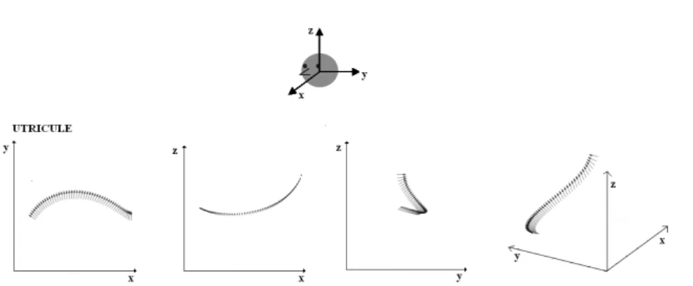
Fig. 3 From left to right are shown the horizontal, sagittal, frontal and three dimensional views of the vectors representing the direction of the kinocilium of the hair cells along the modeled striola of left saccule.

Fig. 4 From left to right are shown the horizontal, sagittal, frontal and three dimensional views of the vectors representing the direction of the kinocilium of the hair cells along the modeled striola of left saccule.

where g(u) represents an arc of circle of center (xc, yc, 0) and radius r.

In the case of the saccule, the curve representing the striola and lying on S2 _{is given by the parametric equations:}

f (u) = u, g(u) = −pR2_{− u}2_{− h(u)}2_{, h(u) = cu}3_{+ ǫu, (8)}

where h(u) is a cubic polynomial.

The equation for the utricular striola reproduces the known convex shape in the horizontal plane and its known anterior upward inflexion. The cubic equa-tion for the saccular striola corresponds to the known inflexion in the sagittal plane and to its medial curvature. The parameters of these curves have been chosen to be similar to available experimental data about the shape of the left utricular ([67], [69]) and saccular striola ([67], [45], [70]) of humans. For the left utricle we have taken: (xc, yc, 0) = (4, 0, 0), r = 5, R = 8 and u ∈ [−1.0, 6.8].

In addition the curve has been rotated of −0.3 radians (−17.19 degrees) with respect the X−axis, of −0.4 radians (−22.92 degrees) with respect the Y −axis

and of −0.5 radians (−28.65 degrees) with respect the Z−axis (see Fig.3). For the left saccule we have taken: c = 0.014, ǫ = 0.01, R = 10 and u ∈ [−5, 5]. In addition the curve has been rotated of −0.53 radians (−30.37 degrees) with respect the X−axis and of π radians (180 degrees) with respect the Y −axis.

In Fig.3 and Fig. 4 are shown respectively the morphological polarization vectors associated to the striola of the utricle and of the saccule on the left side of the head. They correspond to the arrows in Fig.1, where a three-dimensional view of the macular surfaces of the left utricle (a) and saccule (b) are shown together with their morphological polarization vectors. All morphological po-larization vectors on the striola are oriented along the positive Y −axis for the utricle and along the positive Z−axis for the saccule.

The location of hair cells along the striola is computed by taking the arc length l(u) of the curve C,

s = l(u) = Z u

0 k C

′_{(v) k dv, (9)}

where C′ _{is the velocity vector of the curve C. By using s as new parameter,}

the curve C can be written as:

C : s 7→ (F (s), G(s), H(s)), (10)

where s varies in [smin, smax] ⊂ R and where F (s) = f(l−1(s)), G(s) =

g(l−1_{(s)) and H(s) = h(l}−1_(s)).

In the following we consider that several hair cells can have the same param-eter s, thus we model a narrow band of cells and not only a one-dimensional array of cells, but we neglect the effects of the width of the band.

The discretized version of the curve C consists of a finite set of equidistant points C = {C(0), C(L

N), ..., C( L(N −1)

N )}, where N = 50 is the number of

mod-eled hair cells and L is the length of the curve C. In the following we denote by si the parameter (i − 1)_NL for i = 1, ..., N .

The curve C is equipped with a vector field N(s) normal to the tangent T(s) of C and tangent to S2_{. If we denote by R(s) the vector normal to S}2_{, the vector}

field N(s) is obtained as the normalized vector product: N(s) = _kT(s)×R(s)kT(s)×R(s) . The sign of N depends on the signs chosen for T and T and on the orientation OXY Z. We adapted these choices in such a manner that the vector field N(s) represents the morphological polarization vectors along the striola.

3.3 Response of single hair cells

We assume that the type I hair cells along the striola have non-linear receptive fields, which make them more sensitive to acceleration vectors orthogonal to the striola than a cosine tuning would predict. This is compatible with the simulation results of Nam et al. [47], that we will consider in section 5.

Denoting by A the linear acceleration of the head, we call αi= α(si) the

angle between A and the vector Titangent to the curve C at the point si, and

βi = β(si) the angle between A and the vector Ninormal to the curve C and

tangent to the surface of the sphere at the point si∈ C.

The response of a single hair cell of parameter sito the acceleration stimulus

Ais given by the product of two functions:

R(si, A) = f1(αi)f2(βi). (11)

The function f1 expresses the dependency of the instantaneous response

of a single hair cell at C(si) with respect to the angle αi. We choose f1(αi) as

follows

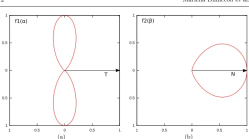
f1(αi) = sin8(αi). (12)

This function (see Fig.5 (a)) is defined in [−π, π] and assumes maximum value when αi = π₂ and αi = −π₂. This means that f1(αi) is maximum when the

acceleration vector lies on the plane normal to the tangent to the striola at C(si). The exponent 8 was chosen to introduce a strong non-linearity in the

transversal tuning of the hair cell. The modeling study of Nam et al. [47] re-ported a non-linear behavior of this kind, with a flat minimum of the response for right angle stimulations. However, our equation does not model the re-ported symmetric plateau around the angle of maximum response.

The function f2 expresses the dependency of the instantaneous response

of a single hair cell of parameter si with respect to the angle βi. We choose

f2(βi) as follows f2(βi) = 1 2cos(βi)(1 + erf (3( π 2 − 0.4 − βi))), (13)

where erf is the error function erf (z) = √2

π Z z

0

e−t2dt. (14)

This function (see Fig.5 (b)) is defined in [0,π₂] and assumes maximum value when βi= 0. Therefore, the response is maximum when the acceleration

vec-tor has the same orientation of the morphological polarization vecvec-tor Ni. It

represents the standard cosine tuning in the polarization direction.

Therefore, in the plane normal to the striola, the response R(si, A) is

max-imum when the acceleration vector A is oriented to the kinocilium.

The proposed activation function does not take into account the intensity of the acceleration A: a complete model should introduce a sigmoid function σ with a threshold, for measuring the dependency in the norm a = kAk, giving:

e

R(si, A) = σ(af1(αi)f2(βi)). (15)

However, in the present study this dependency on the norm and the static non-linearity have little importance, being the acceleration direction the cru-cial element in the analysis.

1 0.5 0 0.5 1 1 0.5 0 0.5 1 f1(α) T 1 0.5 0 0.5 1 1 0.5 0 0.5 1 f2(β) N (a) (b)

Fig. 5 (a) Tuning function f1(α) which models the response of a single hair cell si to an

acceleration stimulus, whose direction forms an angle α with with the vector tangent to the striola at si. (b) Tuning function f2(β) which models the response of a single hair cell sito

an acceleration stimulus, whose direction forms an angle β with the vector normal to striola and tangent to the surface of the macula at si.

3.4 Response of calyces afferents 3.4.1 Single afferent response

We assume that the striolar afferent neurons integrate non-linearly the activ-ities of two hair cells on average.

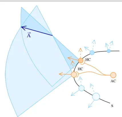
The majority of the hair cells in the striolar region of the macula have the particularity of being totally surrounded by a nerve calyx. In our simplified model each afferent neuron takes information from two calyces. We argue that striolar afferents proceed by estimating the acceleration directions as intersec-tion of dihedral sectors, being each sector associated to one of the hair cell captured by a calyx ending of this afferent. Fig.6 shows how the theoretic preferred direction of the afferent aij capturing two hair cells of parameters si

and sj is computed geometrically. To each parameter si is associated a plane

determined by its polarization vector Ni and the vector Ri normal to the

surface of the macula at C(si). The preferred direction of the afferent aij is

given by the direction of intersection of the planes associated to each hair cell it captures.

For each possible afferent cell aij, the theoretic preferred direction Aij =

(θij, φij) is given by the vector product T_i×Tj kTi×Tjk.

The response to a given acceleration stimulus A of a single afferent aij

A

HC HC

s

AC

Fig. 6 An afferent cell (AC) encapsulates in calyces two hair cells (HC) on the striola (s). The preferred direction A of the AC is given by the intersection of the planes associated to each hair cell, being each plane determined by the polarization vector of the hair cell and by the vector normal to the surface of the macula at the point representing the hair cell.

the product of the responses of the two hair cells:

R(aij, A) = R(si, A)R(sj, A) = f1(αi)f2(βi)f1(αj)f2(βj) (16)

Therefore, the response of a single afferent is given by the intersection of the set of directions that cause an important excitation of each hair cells.

The dynamic response of the afferent aij to the acceleration stimulus A

would be described by the following equation: R(aij, A)(t) = Z f1(αi(t′))f2(βi(t′))f1(αj(t′))f2(βj(t′))δǫ′(t − t′)dt′, (17) where δ′ ǫ(t −t′) = dtd( 1 √ 2ǫe− |t−t′ |2

2ǫ ), with ǫ > 0 is a time wavelet approximating

the derivative of the Dirac function. This formula would make the afferent cell able to detect changes of acceleration directions. However, in the following we will only consider the region of acceleration directions and the variations of these directions seen by the afferent cell without testing the response to dy-namic stimuli. Roughly speaking, the afferent cell would compute the discrete

derivative A(t+δt)−A(t)_δt whereas we consider only the response to A(t) and A(t + δt) separately and we check if the difference between the two responses is large (see section 4.2.3).

In section 5 we present justifications for this kernel, from the known physiology of striolar afferent neurons [14], and from analogy with the global response of semi-circular canals afferent neurons [26].

3.4.2 Selection of the population of afferent neurons

From the above striola model equations, we have determined a population of afferents able to detect accurately the variations of linear acceleration. The de-tails of the population selection are given in the section 4, but we expose now the principle underlying our method. We started with all possible pairs of hair cells along the striola: this gave a population of afferent P. Then we computed the domain Ω of acceleration direction which are detected above a threshold (half of the maximum response), and we selected a sub-population Presp of P,

detecting acceleration in Ω above the same threshold. To proceed further we considered the variations of responses when the acceleration stimuli vary, for sensing the linear jerk. We selected a new domain Ω′ _{of acceleration vectors}

Ak such that the gradient of some afferent response was sufficiently high in

one of six directions Vd

k orthogonal to Ak. Then we defined the

subpopula-tion Pgrad of Presp which can detect accurately the variations of acceleration

vectors in sufficiently many directions. We limited the population Pgrad by a

uniformity condition, requiring that the number of afferents sensing a given variation (Ak, Vdk) do not departs too far from the mean number.

3.5 Decoding

Based on the response of a population of afferent cells to a given acceleration direction A, the brain should be able to extract an estimate ˆAof the under-lying encoded original stimulus A. To verify that the information encoded by our model can be appropriately decoded by the brain, we have used a super-vised learning method.

A simple decoding method without learning such as population vector decod-ing proposed by Georgopoulos [20] would be inappropriate in our case, because this decoding method works well when the patterns of activity as a function of the stimulus behaves like gaussian functions. But in our model the patterns of activity as a function of the stimulus parameter do not follow gaussian-like laws (see 4.2).

A learning algorithm was therefore necessary to discover a regular mapping between the population responses and the underlying stimulus. We have used a supervised learning algorithm, the classical backpropagation algorithm with a 2-layer perceptron [2], in order to map the simulated afferent inputs to the direction outputs. Because this algorithm does not use local learning rules, its

biological plausibility remains uncertain, and in fact it has been used here as a simple way to assess the decodability, not as a model of any brain operation.

4 Results

4.1 The shape of the striola and the number of calyces

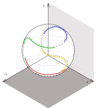
First, our model provides an explanation of the observed shape of the striola, namely a 3D curve with curvature and torsion. This is discussed in details in the mathematical appendix, but we can explain this result without using mathematical symbols. Suppose that an afferent fiber branches and contacts two hair cells along the striola curve S. This will allow an improvement of the information from these two cells as soon as the sectors seen by the hair cells intersect transversally. This implies a large curvature of S. Moreover, in order to get a large solid angle for the possible directions of intersection, the sectors seen by the hair cells have to twist in space, implying a large torsion of S. Due to the known global orientation in space of the maculae ([9], [67], [69], [67], [45], [70]), we obtain a S curve for saccule which has approximately the same disposition in space than the S curve of the utricle of the opposite hemi-sphere of the brain. Thus, on each side of the brain we have two twisted space curves, and by the union of all these four curves we obtain a curve on a sphere that resembles the division on a tennis ball (or suture of base ball) (see Fig. 7). A main point in our model is that the striola afferent system forms a map of directions in space by coupling several points along the striola curve. This correspond to the mathematical concept of divisor of a curve, due to Abel and Riemann (see the book of Griffith and Harris [24]). Since directions in the three dimensional space depend on two parameters and points on a curve depend upon only one real parameter, in average we must take into account two points on the curve for each direction in 3D space. This agrees with ex-perimental observations: the results of Goldberg et al. [22] give 2.26 as a mean number of calyces by afferent in the utricle of the chinchilla, and the results of Desai et al. [12] give 1.84. These last authors also computed the mean number of calyx terminations of afferents for the saccule and utricle of six species of rodents (mouse, rat, gerbil, guinea pig, chinchilla and tree squirrel): except for mouse and gerbil (around 1.55 and 1.65 respectively) they found indexes larger than 1.75.

Thus our model gives an explanation of the observed mean number of calyces for striolar afferent fiber.

As a consequence we conclude that the striolar system can detect three di-mensional acceleration directions and their change in time (jerk) without the need of computing the intensity of the sensed accelerations.

x −y

z

Fig. 7 The red and the yellow curves represent respectively the striola of the right and of the left utricule. The green and the blue curves represent respectively the striola of left and of the right saccule.

More refined theoretical results (see 7) allow an improvement of the optimal curve for the striola:

1) If a curve S allows a smooth parametrization in an open solid angle by pairs of points in the vicinity of a point P0, then there exists an Euclidian

affine change of coordinates in the three dimensional space such that S has a contact of order 4 with a twisted cubic.

2) Let us choose as coordinates for the pairs of points on the curve S the elementary symmetric functions of the curvilinear abscissas, and as measure on the set of directions the Euclidian solid angle. Denoting by ϕ the trans-formation sending the pairs of points in S to the corresponding directions in the three dimensional space, then, at the second order of approximation in the distance of the points, the jacobian determinant of ϕ is equal to −κτ2_/4,

where κ, τ denote respectively the curvature and torsion of the curve. Thus, for curves S in the three dimensional Euclidian space, to obtain the largest uniformity of representation for information maximization, the curve S must have a curvature and a torsion such that the function τ√κ is constant; 3) For curves on a sphere, the optimal curves are the unique spherical curves with given constant product τ√κ. They are associated to lemniscatic elliptic functions [23].

However, our model does not implement the theoretically optimal striola, but a standard spherical curve with parameters deduced from empirical data.

4.2 The receptive domains

4.2.1 Multiplication versus addition

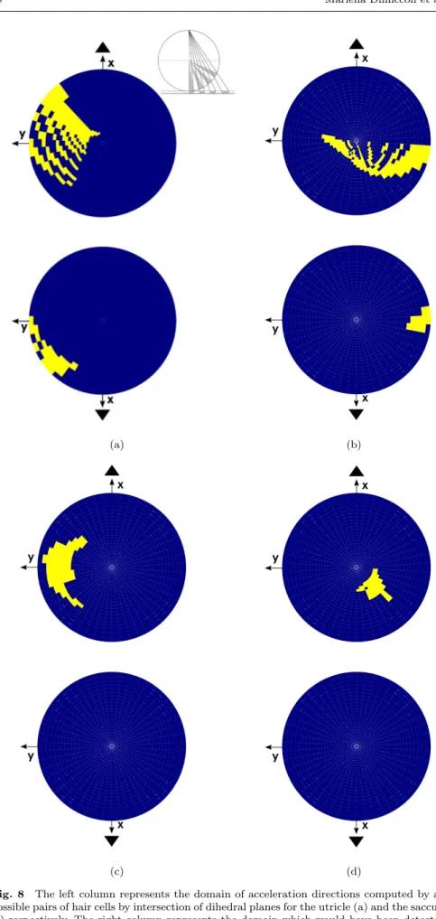
Numerical simulations allowed to compare different rules of cooperation be-tween hair cells. We compared the averaging rule with the intersection rule and we found that the second gives a much larger detected domain than the first, as can be seen on the Fig. 8.

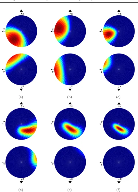
In Fig. 9 is shown an example of receptive field (response in function of ac-celeration direction) of an afferent capturing two hair cells. On the first row of Fig. 9, corresponding to the utricle, are represented the responses of two different hair cells ((a) and (b)) and responses of the afferent capturing these two hair cells (Fig. 9 (c)). The same representation holds for the second row, which corresponds to the saccule.

4.2.2 Responding afferent population

Another result, obtained through numerical simulations, is the domain of ac-celeration directions sensd by the striolar system. This has been achieved by assuming the simple forms of maculae and striolae discussed above and by selecting sub-populations of afferent neurons in order to have an uniform de-tection of the variations of acceleration directions (see Fig. 11).

Let S2

Abe the sphere of radius 1 representing all possible acceleration

direc-tions. In Fig.11 (a) and (b), we have associated to each Ak ∈ SA2 the maximum

value of the response obtained among all possible afferents. As expected con-sidering the orientation of the morphological polarization vectors along the striola (see Fig.1), we have found functional polarization vectors only on the upper hemisphere for the saccule and only on the left part of both upper and low hemisphere for the utricle (see Fig.11).

We denote by Ω the region of S2

A for which the global response is above a

fixed threshold λR:

Ω = {Ak∈ SA2 | ∃aij: R(aij, Ak) > λR}. (18)

We simply took for λRthe half of the maximum absolute value of the response

(a) (b)

(c) (d)

Fig. 8 The left column represents the domain of acceleration directions computed by all possible pairs of hair cells by intersection of dihedral planes for the utricle (a) and the saccule (c) respectively. The right column represents the domain which would have been detected by taking the vector sum of hair cells activity by pairs (b) and (d) for the utricle (b) and the saccule (d) respectively. The apparent checkerboard pattern is due to the discretization of the population. The inset shows how the north (south) hemisphere is represented with a stereographic projection from the south (north) pole on the plane tangent to the north (south) pole.

(a) (b) (c)

(d) (e) (f)

Fig. 9 On the sphere of all acceleration directions, (a) and (d) represent the receptive field of a single hair cell sifor the utricle and the saccule respectively; in the same manner (b) and

(e) represent the receptive field of another single hair cell sjfor the utricle and the saccule

respectively, then (c) and (f) represent the receptive field of the afferent aij capturing the

(a) (b)

(c) (d)

(e) (f)

(g) (h)

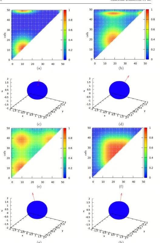
Fig. 10 (a), (b) for the utricle and (e),(f) for the saccule represent the activity of all possible afferents in response to the acceleration stimulus represented respectively in (c), (d) and (g), (h). In (a),(b),(e), and (f) the abscissa and the ordinate represent the 50 cells modeled on the striola and the color code the activity of the target afferent cell getting input from the respective pair of hair cells.

Fig. 11 Maximum value of the response over all possible afferents, normalized with respect to the maximum absolute value, represented on the sphere of all acceleration directions, seen from above and from below, for the utricule on the left column and for the saccule on the right column.

denoted by Presp the set of afferents that respond to at least one acceleration

in Ω with an activity above λR.

Presp = {aij, i 6= j, | ∃Ak ∈ Ω : R(aij, Ak) > λR} (19)

This had the effect of reducing the dispersion of responses without reducing too much the size of the population.

4.2.3 Uniform capture of linear jerk

The acceleration vectors in Ω are sensed with an intensity range that goes from λRto the maximum absolute value. As it can be observed in Fig.11 ((a)

and (b)), the capture is quite uniform in this region. However, since our hy-pothesis is that the afferents along the striola are best suited to capture the variations of acceleration directions (to sense the jerk), what really matters is that the capture be uniform with respect to a variation of the acceleration directions represented in Ω. Let us describe how we have selected a subset of Ω and a sub-population of Presp to this goal:

First we computed how well a given afferent aij in Presp is able to detect the

Vk:

For each acceleration Ak ∈ Ω, we have considered a set of six gradient

ref-erence directions Vd

A_k, d ∈ {1, .., 6}, randomly chosen and forming a

regu-lar hexagon. Note that for each acceleration Ak the set of VdA_k lies on the

plane perpendicular to Ak. We associated to each acceleration Ak ∈ Ω and

to each afferent aij ∈ Presp the unitary vector gradient ∇Ak R(aij,A)

k∇AkR(aij,A)k, where

k∇AR(aij, Ak)k is the norm of the gradient of R(aij, Ak) with respect to the

acceleration direction Ak. k∇AR(aij, Ak(θ, φ))k = s (∂R(aij, A(θ, φ)) ∂θ ) 2_{+ (}∂R(aij, A(θ, φ)) ∂φ ) 2 1 cos2_(θ), (20)

where we take the discretization: ∂R(aij, A(θ, φ)) ∂θ = R(aij, Akθ(θ + δθ, φ)) − R(aij, Ak(θ, φ)) δθ (21) and ∂R(aij, A(θ, φ)) ∂φ = R(aij, Akφ(θ, φ + δφ)) − R(aij, Ak(θ, φ)) δφ (22)

We defined ν as the maximum among all possible afferents in Presp of the

minimum value of the gradient with respect to an acceleration variation among all accelerations in Ω:

ν = max

aij∈Presp

min

A_k∈Ωk∇AR(aij, Ak)k (23)

For each gradient response ∇A_k(R(a_ij, A_k)) whose norm is above ν, we

mea-sured its proximity to the gradient reference direction Vd

A_k by computing the

angle ω = arccos(∇A_k(R(a_ij, A_k)) · Vd_A k)).

We determined that a variation of Akin the direction VdA_kis well detected by

aij if ∇A_k(R(aij, Ak)) ≥ ν and ω < π₆. These criteria were retained to insure

a sufficiently dense detection of the variations of acceleration directions. The acceleration vectors appearing for at least one pair aij, V form a solid

angle Ω′ _{inside Ω, and the afferent appearing for at least one pair A, V form}

a subset P′ _{of P} resp.

If the gradient direction Vd

A_k is well detected by an afferent cell the

gradi-ent direction Vd+3A_k will also be well detected, because its scalar product with

the gradient has the same absolute value and the opposite sign. Therefore the six gradient directions correspond to three independent gradient orientations. The choice of considering only three independent gradient orientation instead of four or more is due to the limited number of hair cells (50), and therefore possible calyx afferents, modeled in the simulations. Nevertheless, we have ver-ified that even when considering six gradient orientations instead of just three

(that is twelve directions), the afferent cells are well distributed along all these six orientations.

For each afferent aij we computed the number Nij of times that aij appears

as good detector of a variation of acceleration in Ω′_{. We defined a threshold}

λN as half of the maximum of the numbers Nij over all pairs i, j. The role

of this threshold is to prepare a population of afferents with uniform ability to detect the linear jerk. Then, for each Ak ∈ Ω′ we defined the set PA′ _k by

asking that aij belongs to P′ and that the corresponding Nij is larger than

λN. And we defined Pgradas the union of the sets PA_k over A_k∈ Ω.

The final step consists in verifying that all the subsets PA_k contain almost

the same number of elements in Pgrad. This corresponds to our uniformity

condition.

More precisely, we consider the set of elementary events given by the pairs (Ak, Vdk) where Ak belongs to Ω′ and d varies from 1 to 6, and we define the

random variable N as the number NA_k,Vd

k of afferents aij in Pgrad that are

good detectors of the pair (Ak, Vdk). Then we define µA_kas the mean over the

variations, µA_k= 1 6 6 X c=1 NA_k,Vd k; (24)

the mean µ of N is given by

µ = 1 M M X k=1 µA_k (25)

and the standard deviation σ of N is given by σ = v u u t 1 M M X k=1 (µA_k− µ)2 (26)

The inequality of Cantelli (also known as the one-sided inequality of Cheby-shev), guarantees that in almost every data sample, no more than _1+r12 of the

data values can be more than r standard deviations away from the mean. In formulas, if µ is the expected value of the random variable N and if σ2_denotes

its variance, than for any real number r > 0, the inequality of Cantelli is

Pr(µ − N ≥ rσ) ≤ _{1 + r}1 2. (27)

We found that, for the population Pgrad, the numbers NA_k,Vd

k satisfy the

in-equality µ − NA_k,Vd

k ≥ rσ for a value of r equals to r = 3 in the case of the

utricle and equals to r = 1 in the case of the saccule. We computed µ−rσ = 38 for r = 3 for the utricle and µ − rσ = 23 for r = 1 for the saccule.

The tables on Fig. 4.2.3 show the statistics of N computed on the population Pgrad for the utricle and for the saccule.

UTRICULE min µAk 58 max µAk 141 min σ2 Ak 0.000000 max σ2 Ak 0.333333 min µnorm Ak 356.256717 max µnorm Ak 1752.198653 min (σ2 )norm Ak 0.000001 max (σ2 )norm Ak 0.180787 µ 96.510689 σ 21.614370 SACCULE min µAk 2 max µAk 82 min σ2 Ak 0.000000 max σ2 Ak 0.333333 min µnorm Ak 1010.276078 max µnorm Ak 2901.018712 min (σ2 )norm Ak 0.000002 max (σ2 )norm Ak 0.049325 µ 42.178899 σ 19.057136

Fig. 12 Statistics computed on the population Pgradfor the utricule and for the saccule.

The superindex norm means that the statistics have been computed taking into account the norm of the reference vectors Vd

Ak and the vector Akinstead of their direction.

4.3 Decoding by learning

We considered a neural network to which are provided Nstraining examples.

Each training examples is a pair (pk, tk), where pk is a pattern vector of activities and tk _{is the corresponding target vector with k ∈ [1, N}

s]. Let np

be the number of elements of each pattern vector and nt be the number of

elements of each target vector. In our model np corresponds to the cardinality

of the set Pgrad, that is np= 770 for the utricle and np= 563 for the saccule,

and ntcorresponds to the components of the acceleration vector, that is 2 in a

spherical coordinate system. Each element pk

m of an input vector corresponds

to the response of the neuron m to the corresponding target vector tk_{: p}k m=

R(am, tk) = R(am, Ak). Therefore each training example is a pair having the

form: ([R(a1, Ak), ..., R(anp, Ak)], [θk, φk]), where (θk, φk) are the components

of Ak. Let w np×nh

1 be the matrix of synaptic weights between the neurons of

the input layer and the neurons of the hidden layer and wnh×nt

2 be the matrix

of synaptic weights between the neurons of the hidden layer and the neurons of the output layer.

We stopped the learning algorithm when the average quadratic error between inputs and outputs attained a fixed threshold ǫ = 10−5_.

Once obtained the matrices of learnt weights w1and w2, an estimate ˆAof the

stimulus A can be obtained by using the following formula:

ˆ A= nt X l=1 Ψ ( nh X n=1 w2[n][l]Ψ ( np X m=1 w1[am][n]R(am, A))), (28)

where Ψ denotes the arc-tangent function. We have tested the goodness of the learnt weights over the entire set of accelerations in Ω′ _{and we have evaluated}

the outcome by calculating the angle between the vectors A and ˆA. We found that the average error for a trial is less than one degree.

In the region where the slope of the arc-tangent function can be approximated to 1, we can re-write equation (28) in linear form as:

ˆ A= nt X l=1 nh X n=1 w2[n][l] np X m=1 w1[am][n]R(am, A); (29)

and we can rewrite this equation as: ˆ A= np X m=1 AmR(am, A), (30) where Am=Pnl=1t Pnh

n=1w2[n][l]w1[am][n] represents a new adapted preferred

direction associated to the afferent cell am.

4.4 Testing the robustness with respect to neuronal noise

To test the robustness of our model with respect to neuronal noise, at each iteration of the BPNN algorithm, we have sampled the value of the response

˜

R(am, Ak) of each afferent am to the acceleration direction Ak from a

gaus-sian noise distribution with standard deviation σ = 0.1 and centered at µ = R(am, Ak): ˜ R(am, Ak) = √ 1 2πσ2exp (q − µ)2 2σ2 , (31)

where q is a random value in the range [0, 1]. Experimental simulation have proved that the network is able to learn the right weight in presence of neu-ronal noise so that the error is still of the order of five degrees.

4.5 Comparison

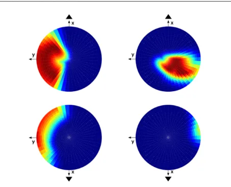
In Fig. 13 (right) are shown the functional polarization vectors measured ex-perimentally by Fernandez and Goldberg [16], as well as the distribution of morphological polarization vectors of the hair cells computed by the model of Jaeger et al. [29] for the utricule (up) and for the saccule (down). Before comparing them to the domain of acceleration directions we obtained (see Fig. 13 (left)), we recall that the experimentally recorded afferent vectors in-clude all type of afferents, calyces, dimorphic and boutons, that are distributed along the overall macula. In addition, the simulated density of morphological polarization vectors includes type I and type II hair cells, distributed along the overall macula. On the contrary, the results shown in Fig. 13 (left) have been obtained by modeling only calyces striolar afferents. In principle, our re-sults, which relate directly to afferents, should be compared with the data of Fernandez and Goldberg, more than to the simulations of Jaeger et al., which

considered single hair cells responses, rather than integrated afferent responses. We found a big similarity between our computational results and the experi-mental results of Fernandez and Goldberg, and a large overlap with Jaeger et al. modeling results. The dissimilarities can easily be explained. As stated in section 4.2.2, the fact that we have taken into account only the morphological polarization vectors along the striola (see Fig.1) explains why we find func-tional polarization vectors only on the upper hemisphere for the saccule and only on the left part of both upper and low hemisphere for the utricule. Taking in account the observation of Songer (see [14]), we would have to symmetrize the domain for the saccule with respect to the center of the sphere.

The observed similarity is a non-trivial result, since Fernandez and Gold-berg registered afferents from all the maculae surfaces. Thus this confirm our suggestion that striolar and extrastriolar regions cover two similar head accel-eration domains, but at different orders of dynamics.

5 Discussion

In the present study we obtained an explanation of the three dimensional shape of the striola on the otolith maculae and we predicted the range of linear ac-celeration directions, including gravity, whose variation is well detected by the striolar system. Our model was based on hypotheses about the function of striolar type I hair cells, about the way afferent cells collect information from them, and about the function of the afferent population. However, this theo-retical study and its computational test were based on several simplifications that we discuss in this section, in the light of previous experimental data and computational models.

The main line of thought we followed was that the function of the striolar region is to give maximum possible information about the most dynamic move-ments of the head, that is rapid, phasic and high frequency information. By essence this information is three dimensional but it has to come from specific morphology and physiology of cells concentrated in a narrow region. There-fore cells from distinct places of the striola have to share their information. The starting hypothesis was that striolar afferent neurons, either dimorphic or calyces, choose their preferred acceleration direction according to the in-tersection of domains chosen by their calyces. We suggested that one afferent counts for two hair cells in the mean, and detects acceleration by intersection of the preferred planes of the contacted hair cells. This is a doubly non-linear process: type I hair cells must have a non-linear tuning, not cosine but plateau, and afferents must react to as a product, not as a sum or a mean of hair cells. In this model, the effective dimension of the whole striolar system is not one, as would predict a narrow band, but it is two, as if it were a supplementary macula surface.

Fig. 13 In this image are shown the stereographic projections of the unit sphere, with the upper hemisphere in the upper row and the lower hemisphere in the lower row. In the left image, for the utricule as well as for the saccule, is shown the maximum value of the response over all selected afferents for each acceleration direction, normalized with respect to the maximum absolute value. In the right image, for the utricule as well as for the saccule, is shown the density of the morphological polarization vectors along the macula modelized by Jaeger et al. [29]. They increase from white over gray to black and were normalized with respect to the largest density found on one of the epithelia. Superimposed on the projections,are also shown polarization vectors found experimentally in single cell recordings from the vestibular nerve of squirrel monkeys by Fernandez and Goldberg [16].

Then we can conjecture that sudden acceleration direction changes provoke a shape of activation along the striola with several maximum points (in aver-age two). This is supported by the model of Jaeger and Haslwanter [28]: ”... peak responses occur simultaneously on different locations of the striola.” We do not exclude the possibility that different processings happen in the saccule and in the utricle (Ross et al. [56], [53]), but we suggest a common geometric principle for acceleration and jerk detection in a large domain.

In addition our model gives three testable predictions:

The first prediction deals with the biophysical properties of the transduction. We predict that the reaction of the type I hair cells in the striolar region is not well fitted by a cosine tuning of the angle with the polarization vector. More precisely, we suggest that a stimulation exerted transversally to the plane of symmetry of the hair bundle (i.e. the plane which is generated by the polar-ization vector and the normal to the macula), generates a rapidly decreasing reaction, giving zero at an angle less than 90 degrees. On the contrary, a stim-ulation exerted transversally to the macula generates a cosine decreasing of the reaction of the hair cell.

The second prediction deals with the neural signals in the vestibular nerve. We predict that the afferent neurons on the striolar region react non linearly to the input of the type I hair cells they contact. The exact form of the re-ceptive field would be given by a multiplicative formula of the reactions of the hair cells it connects (as a probability of independent events). This hypothesis could be tested by neurophysiological recordings. For the moment we do not know any direct evidence supporting this prediction.

The third prediction concerns the information flow in the afferent vestibu-lar nerve. We predict that the striovestibu-lar afferents sense a domain of acceleration as large as the domain sensed by the extrastriolar afferents. However, at least for the utricle, where only one polarization vector occurs along the striola, the receptive field is unilateral, i.e. only medio-lateral excitation occurs for the striolar afferent system. Note that the four striolae together construct a fairly complete mapping of the acceleration domain (see 7). Amazingly, there is a blind angle directed downward, which was also present in the data of Fernan-dez and Goldberg.

Several existing results help to justify the assumption we made on the hair cells: first, the specificity of striolar bundles compared to extrastriolar bun-dles was established by Peterson et al. for turtle’s utricle, [43], [57], [58], [73]). In particular the type I cells in the striolar region have more numerous and thicker stereocilia, with steeper slope, smaller ratio of kinocilium height over highest stereocilium height (KS), making them adapted to higher frequency tuning. In addition these cells have particularly wide bundles in the direction of the tangent to the striola, i.e. parallel to the PRL. These properties were confirmed in rodents by Li et al. [35]. According to [38], in mammals, the striolar bundles are wing shaped with more stereocilia along the axis orthogo-nal to the sensitivity axis, but bundles of peripheral cells are more round and

compact. Phasic responses are expected for these wider hair bundles, which accords with a broader detection of acceleration directions. Our assumption on the hair cell receptive field are justified by the simulation results of Nam et al. [47]: using parameters of striolar hair cells bundles, in particular transversal wideness, the authors found a plateau around the best response and a non-linear sudden decreasing of the depolarization of the hair cell for transversal stimulations. Of course, to confirm the stability of our model we have to test a more general non-linearity than sin8_{(α), but the mentioned studies give a}

direct justification of our assumption. However our precise hypothesis that the striolar type I hair cells detect a plane more than a direction has to be directly verified in situ.

The fact that the receptive fields of hair cells are large in the striola is com-patible with the rapid reaction of the striolar system.

The reported afferent cell receptive fields do not have the same kind of non-linear properties: on the contrary, a non-zero response of afferent neurons is observed for transversal stimulations, 15/100 according to Fernandez and Goldberg [16], [17], [18], and from 4/100 for regular to 8/100 for irregular afferents, in gerbil [13], or pigeon [60]. Rowe and Peterson [58] discussed the origin of this behavior and proposed the hypothesis that the residual response comes from the diversity of the preferences of the contacted hair cells. Note that the majority of afferents have bouton contacts with type II hair cells in addition to their calyces, so that the enlargement of their receptive field could come from these type II cells as well as from type I cells.

The central functional hypothesis of our approach is that multiple calyces allow an afferent neuron to ”multiply the reaction of hair cells”, as do a coin-cidence detection in the spatial domain or in the temporal domain. The idea is that along the striola there is more statistical independency among hair cells integration, which accords with the large distances between these cells and the distribution of small otoconia above the striola [72], resulting in a multiplicative joint distributions for the activity of the afferent cells.

Thus we suggest that striolar afferents proceed by elimination, intersect-ing a set of incomplete sources of information, primarily comintersect-ing from type I hair cells that are biased to detect planes of directions more than individual directions. We can say that afferent neurons signal a probability of accelera-tion (or acceleraaccelera-tion change) proporaccelera-tional to the product of the individual probabilities of connected hair cells. This could make them bayesian esti-mators of motion from conditionally independent sources: P (A|H1, H2, ...) =

P (H1|A)P (H2|A)...P0(A)/P (H), where the variable A denotes the

acceler-ation direction, the variable H = (H1, H2, ...) denote the set of hair cells

re-sponses, and P0(A) denotes the a priori probability on the acceleration. The

denominator P0(A) is necessary in the above Bayes formula; it is the total

probability on the stimulus A. The a priori probability could be uniform, but a much more interesting assumption is that the efferent system and the type II hair cells modulate this a priori knowledge. For a recent discussion of the

application of Bayes inference to neural systems see [71].

The hypothesis that the afferent population detects the variation of accel-eration direction as uniformly as possible, corresponds to the maximization of the information on the change of movement direction or gravitation direction. Known results (see [22] and [14]) support the fact that striolar afferents are efficient for a dynamical detection, transmitting a signal between the jerk and the acceleration of the head. To effectuate such a derivative in time we hypothesized a kernel represented by a Riemann-Liouville integral, i.e. a frac-tional derivative of a delta function (cf. equation (17) in section 3). Thus we assume that the neurophysiology of afferent cells, probably helped by calyces synapses, is able to reverse the integration into a differentiation. A convincing argument for this derivative function comes from the results of Highstein et al. [26] on the afferent neurons to the cristae of semi-circular canals, where it was established that the gain and the phase both increase with the frequency of the stimulation for frequency after 5-10Hz, which cannot be due to the biomechanics of the semicircular canals and the cupula [50]. Thus this effect is probably due to the physiology of hair cells and afferent cells.

Ross et al. [55] have investigated the morphological basis for directional sensitivity of vestibular afferents receiving several hair cells. They agreed with Tomko et al. [68] to discard a simple averaging process. More recently Ross et al. [56] have elaborated a three dimansional finite volume model of calyces and ribbon synapses to study the effect of changing geometry of calyces, lo-cation and number of synapses, directional input, and activation timing. This computational tool could be used to verify our assertion. More generally it is evident that a more elaborate three dimansional computation is needed to give a better test of our model and its robustness.

In our computational study we have considered type I hair cells perfectly ar-ranged along a curved line, and afferent cells contacting exactly two hair cells. In reality, the striolar region is extended, the polarization vectors of the hair cells have a large variability, and the afferents in their majority contact also type II cells, moreover some afferents enclose only one hair cell, and some oth-ers enclose three cells or more. How can we manage this variability and this complexity?

Note that, in our model, each place along the striola curve counts for several type I cells, because it represents as many hair cells the selected afferents con-tacting this place incapsulate. Thus the striola curve in our model represents a narrow band around the striola on the macula.

Although it would be important to introduce more variability in our model, for example using a random processing in place of a simple geometric model, in the present study we do not add any detail that could by itself have strong correcting effects.

sim-ple princisim-ples and augments the information flow.

5.1 Limits of our model

First, the division of the striolar region on the saccule by the PRL (mentioned in [14]), seems to be contradictory with the assumption of continuity of the polarization. However, in birds the striola possesses this kind of structure on both the utricle and the saccule, but the studies of Dickman et al. [61], [74], show that in this case the afferent neurons contact hair cells on the same side of the PRL, and that the true striola is made of two components.

Second, the majority of striolar afferents contact type II and type I hair cells, but we never have used this overlapping in our model. It could be pos-sible that type II hair cells are responpos-sible of a better precision in sensing the preferred direction of the afferent neurons. Also they can participate in the regulation of gKL conductances which is necessary for the activation of

synapses in calyces. Another natural idea for the contribution of type II cells to the information processing along the striola is that that they could be very helpful to take into account the intensity of the sensed acceleration vectors. In fact, in our model we have only considered acceleration directions, in par-ticular it was the only element considered for population selection, but the intensity should be considered in any functional test.

Third, the irregular dynamics of the striolar afferents is an essential prop-erty for the vestibular information flow, but we did not model it, as it could be (see [63]). The true selection of a subpopulation for jerk detection should be done by including the dynamics. Thus more computational work has to be done to obtain a complete proof of our model. A complete model should take into account hair cells bundles and polarization variability, the complex geometry of the striolar region, the modeling of calyces terminations, the ion channel kinetics of the hair cells and of their afferents, the modulation by type II cells and the propagation of spike trains along the afferent axons.

5.2 Phasic and tonic information

Our model fits well with the hypothesis of the existence of a phasic, irregular, high frequency adapted, striolar sensory subsystem, responsible for linear jerk detection and short latency vestibular information processing.

As otolith end organs and semi-circular canals conjugate their message in the vestibular nuclei, the striolar system information must be combined with a corresponding canal afferent subsystem. Such a subsystem was described in the center of the crista ampullaris, with comparable physiological characteris-tics although not identical, responsible for detecting rotation acceleration (see [16],[17][18]).

However, the set of afferent dendrites contacting otolith maculae and canals cristae forms a complex parallel processing of presynaptic micro-circuits, with type I terminations regulating type II dendrites, as explained by Ross ([52],[54]). Thus the irregular subsystem must not be confounded with the subsystem of pure calyx afferent neurons. In particular, in mammals it has been shown that type I hair cells are found everywhere on the maculae and on the cristae (see [37]), and that dimorphic connections, mixing calyces and boutons, are largely dominant. In fact, the dynamical properties of phasic-irregular afferent neu-rons, having a gain which augments with the frequency, depend more on the position of their projections with respect to the macula than on the type of contact (see [19]). This is true for otoliths and for semi-circular canals. Besides, it was observed that irregular and regular afferents of otoliths and of canals do not generate completely separate flows in the central vestibular organs (see Boyle et al. [3], Peterson [48], Goldberg [21]). Their projections overlap considerably in the vestibular nuclei. They both contribute to the vestibulo-ocular reflex (VOR) and vestibulo-collic reflex (VCR), that stabilize gaze and head respectively, although the irregular input is more involved in the VCR than in the VOR and the reverse is true for the regular input (see [42], [3]). In frogs, phasic and tonic activities in the vestibular nuclei are segre-gated, but this could be not strictly the case in mammals (nor amniotes) (see [66], [15]). However, the phasic primary vestibular information of otoliths and canals)can generate short latency responses, participating to synchronization in motor control, posture and autonomic modulation. For instance, the jerk information on translation is implicated in early ocular compensation (com-pensatory nystagmus), [5], [25], or in subjective vertical assignment [39]. For birds, experiments of Jones et al. [30] on chicken described a net jerk inten-sity signal, whereas for mammals [32] a fractional order jerk signal (between acceleration and jerk) is reported.

The suggestion we have deduced from our present model of the striola, namely that phasic and tonic vestibular afferents cover the same geometri-cal fields but at different dynamigeometri-cal and frequency domains, is in favor of overlapped information flows between phasic and tonic pathway, but where different contexts should decide of different ranges of contributions of these pathways for integrated adaptation.

5.3 Evolution of the striola complex

Our model can have also an interest from the point of view of evolution. It does not apply to most fishes but it applies to mammals and only partially to birds.

During the evolution of amniotes, the contact with the earth has gener-ated a variety of somato-sensory and proprioceptive information sources to control posture and motion. However, during rapid locomotion the instabil-ity of transient contacts makes the somato-sensory information difficult to be