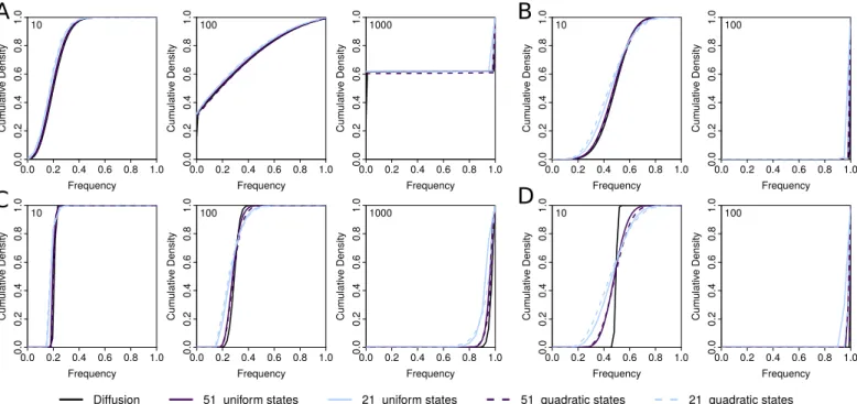
Figure S1Comparison of different grids.Shown are the cumulative probability density distributions (CDF) of allele frequencies after 10, 100 and 1000 generations (shown in top left corner) of selection and random drift starting from a frequency of 0.2 and obtained under the Wright-Fisher diffusion (black) and the mean transition time approximation for 51 and 21 uniform (solid) or quadratic (dashed) states. Results are shown for small (N=100, A and B) and large (N=10, 000, C and D) population sizes and weak (s=0.01, A and C) and strong (s=0.3, B and D) section.
1
2
3
4
5
0
5
10
15
20
Index
Density
log
10(
N
)
P
oster
ior density
Index
0
0
10
20
30
log
10(
N
)
=
2
Index
0
0
10
20
30
Index
0
0
10
20
30
−0.15
−0.05
0.05
0.15
s
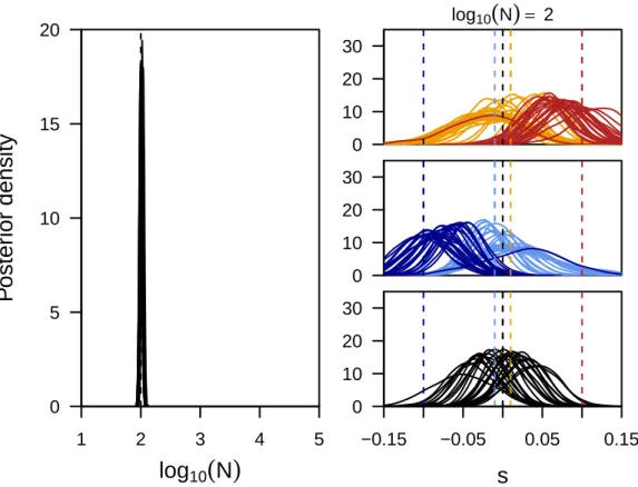
Figure S2Power to infer selection and population size jointly.Here we show the posterior distributions on the population size (first panel) and locus-specific selection coefficients obtained for five replicate simulations for each of three different population sizes. For each replicate we plot the posteriors of all loci simulated under selection (color) as well as five neutral loci picked at random (black). In contrast to the results shown in the main text, the data was simulated here with more ideal starting frequencies, namely 0.1, 0.5 and 0.9 for positively selected, neutral and negatively selected sites, respectively.
1 2 3 4 5 0 5 10 15 20 Index Density log10
(
N)
P osterior density Index
0 0 10 20 log10(N)= 2 Index 0 0 10 20 Index 0 0 10 20 −0.15 −0.05 0.05 0.15 s Index 0 0 20 40 log10(N)= 3 Index 0 0 20 40 Index 0 0 20 40 −0.15 −0.05 0.05 0.15 s Index 0 0 50 100 150 log10(N)= 4 Index 0 0 50 100 150 Index 0 0 50 100 150 −0.15 −0.05 0.05 0.15 s
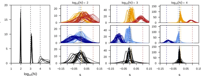
Figure S3Power to infer selection and population sizes jointly.Here we show the posterior distributions on the population size (first panel) and locus-specific selection coefficients obtained for five replicate simulations for each of three different population sizes. For each replicate we plot the posteriors of all loci simulated under selection (color) as well as five neutral loci picked at random (black). In all simulations, starting frequencies were chose randomly for each locus. In contrast to the results shown in the main text, 80% of all simulated loci were affected by selection.
−0.20 −0.15 −0.10 −0.05 0.00 0 10 20 30 40 selection Coefficient s P oster ior Density 201 states 101 states 51 states 21 states −0.15 −0.05 0.05 0.10 0.15 0 10 20 30 40 selection Coefficient s P oster ior Density 0.00 0.05 0.10 0.15 0.20 0 10 20 30 40 selection Coefficient s P oster ior Density −0.20 −0.15 −0.10 −0.05 0.00 0 10 20 30 40 selection Coefficient s P oster ior Density −0.15 −0.05 0.05 0.10 0.15 0 10 20 30 40 selection Coefficient s P oster ior Density 0.00 0.05 0.10 0.15 0.20 0 10 20 30 40 selection Coefficient s P oster ior Density −0.20 −0.15 −0.10 −0.05 0.00 0 10 20 30 40 selection Coefficient s P oster ior Density −0.15 −0.05 0.05 0.10 0.15 0 10 20 30 40 selection Coefficient s P oster ior Density 0.00 0.05 0.10 0.15 0.20 0 10 20 30 40 selection Coefficient s P oster ior Density −0.20 −0.15 −0.10 −0.05 0.00 0 10 20 30 40 selection Coefficient s P oster ior Density −0.15 −0.05 0.05 0.10 0.15 0 10 20 30 40 selection Coefficient s P oster ior Density 0.00 0.05 0.10 0.15 0.20 0 10 20 30 40 selection Coefficient s P oster ior Density −0.20 −0.15 −0.10 −0.05 0.00 0 10 20 30 40 selection Coefficient s P oster ior Density −0.15 −0.05 0.05 0.10 0.15 0 10 20 30 40 selection Coefficient s P oster ior Density 0.00 0.05 0.10 0.15 0.20 0 10 20 30 40 selection Coefficient s P oster ior Density
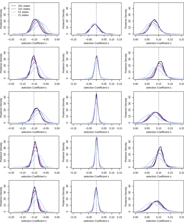
Figure S4Power to infer selection as a function of the number of states.We simulated five independent loci for each of the three selection coefficients s= −0.1, s=0 and s=0.1 for a population size of log10(N) =4. We then inferred the posterior distributions on s for each locus using different numbers of states, but assuming log10(N) =4. Estimates are generally biased towards weaker selection when using too few states.
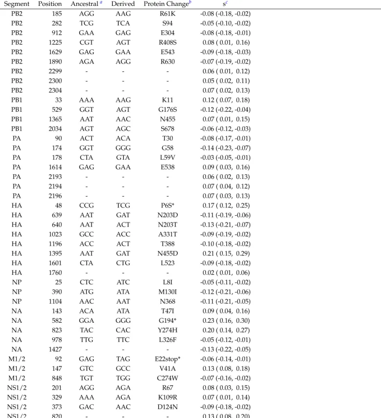
Table S1Sites found to be under selection in Influenza
Segment Position Ancestrala Derived Protein Changeb sc
PB2 185 AGG AAG R61K -0.08 (-0.18, -0.02)
PB2 282 TCG TCA S94 -0.05 (-0.10, -0.02)
PB2 912 GAA GAG E304 -0.08 (-0.18, -0.01)
PB2 1225 CGT AGT R408S 0.08 ( 0.01, 0.16)
PB2 1629 GAG GAA E543 -0.09 (-0.18, -0.03)
PB2 1890 AGA AGG R630 -0.07 (-0.19, -0.02) PB2 2299 - - - 0.06 ( 0.01, 0.12) PB2 2300 - - - 0.05 ( 0.02, 0.11) PB2 2304 - - - 0.07 ( 0.02, 0.13) PB1 33 AAA AAG K11 0.12 ( 0.07, 0.18) PB1 529 GGT AGT G176S -0.12 (-0.22, -0.04) PB1 1365 AAT AAC N455 0.07 ( 0.01, 0.15) PB1 2034 AGT AGC S678 -0.06 (-0.12, -0.03) PA 90 ACT ACA T30 -0.08 (-0.17, -0.01) PA 174 GGT GGG G58 -0.14 (-0.23, -0.07) PA 178 CTA GTA L59V -0.03 (-0.05, -0.01)
PA 1614 GAG GAA E538 0.09 ( 0.03, 0.16)
PA 2193 - - - 0.06 ( 0.02, 0.13) PA 2194 - - - 0.07 ( 0.04, 0.12) PA 2196 - - - 0.07 ( 0.03, 0.13) HA 48 CCG TCG P6S* 0.17 ( 0.12, 0.25) HA 639 AAT GAT N203D -0.11 (-0.19, -0.06) HA 640 AAT ACT N203T -0.13 (-0.21, -0.07) HA 1023 GCC ACC A331T -0.09 (-0.19, -0.02) HA 1196 ACC ACT T388 -0.10 (-0.18, -0.02) HA 1395 AAT GAT N455D 0.21 ( 0.15, 0.29) HA 1601 CTA CTG L523 -0.09 (-0.18, -0.02) HA 1760 - - - 0.02 ( 0.01, 0.06) NP 25 CTC ATC L8I -0.05 (-0.11, -0.02)
NP 390 ATG ATA M130I -0.12 (-0.21, -0.06)
NP 1104 AAC AAT N368 -0.11 (-0.21, -0.05)
NA 143 ACA ATA T47I 0.09 ( 0.04, 0.16)
NA 582 GGA GGG G194* 0.23 ( 0.16, 0.30)
NA 823 TAC CAC Y274H 0.20 ( 0.14, 0.27)
NA 978 TTG TTC L326F -0.05 (-0.12, -0.01)
NA 1427 - - - -0.13 (-0.22, -0.05)
M1/2 92 GAG TAG E22stop* -0.06 (-0.14, -0.01)
M1/2 147 GTC GCC V41A 0.13 ( 0.08, 0.18) M1/2 848 TGT TGG C274W -0.07 (-0.16, -0.02) NS1/2 201 AGG AGA R67 0.08 ( 0.03, 0.15) NS1/2 329 AAA AGA K109R 0.07 ( 0.01, 0.14) NS1/2 373 GAC AAC D124N -0.09 (-0.18, -0.02) NS1/2 820 - - - 0.13 ( 0.08, 0.20)
aAncestral codon refers to the allele with the highest frequency at the beginning of the experiment (passage 0). Dashes indicate mutations in non-coding regions bProtein changes are reported in standard nomenclature but comparing the derived codon to the ancestral codon (not the published reference).