Three essays on portfolio management

Texte intégral

(1) . Three Essays on Portfolio Management. PhD Thesis submitted to the Faculty of Economics and Business Institute of Financial Analysis University of Neuchâtel For the degree of PhD in Finance by. Ivan Guidotti Under the supervision of: Michel Dubois, Professor of Finance, University of Neuchâtel Members of the dissertation committee: Carolina Salva, Professor of Finance, University of Neuchâtel François Degeorge, Professor of Finance, University of Lugano Amit Goyal, Professor of Finance, University of Lausanne Markus Leippold, Professor of Financial Engineering, University of Zürich. Defended in Neuchâtel, October 6th 2015 Faculté des Sciences Economiques Avenue du 1er-Mars 26 CH-2000 Neuchâtel www.unine.ch/seco. .

(2)

(3)

(4)

(5) Acknowledgments. I am especially indebted to Michel Dubois for the guidance and the support he has given to me over the years I spent in Neuchâtel. I am glad that I met such an enthusiastic supervisor, whose discussions, ideas, and trust have stimulated my interests in innumerable ways. I honestly hope that our passionate debates will continue also in the future. I would also like to thank my dissertation committee, Carolina Salva, François Degeorge, Amit Goyal, and Markus Leippold for having kindly accepted to participate to the achievement of this work. Their valuable comments and constructive discussions did contribute to enrich my research and shape my mind. My furthest gratitude goes to Guido Bolliger and Florent Pochon, the persons who kept alive my interest for research during my “Parisian years”. I would like to extend my gratitude to my friend and coauthor Istvan Nagy and all the persons that had an impact on my research through discussions and comments, in particular Stefano Puddu, David Ardia, as well as my Ph.D. student colleagues of the University of Neuchâtel. I also thank this University for having provided me with the resources to work in excellent conditions and to participate to several academic meetings worldwide. I would like to give special thanks also to my closest friends, in particular Filo, Re, Dantun, Matt, and the everlasting circle of Bellinzona. Even if the time we spent together did not directly contribute to improve this dissertation, it allowed me to release the pressure when I crucially needed it. Needless to say, my very first thought goes to my family. I believe I can express the deep and sincere gratitude they deserve only in Italian. Forse non ve ne siete resi conto, ma il vostro sostegno e il vostro affetto in questi ultimi anni é stato cruciale. Silvy, grazie per essermi stata vicina in ognuno di questi giorni, soprattutto in quelli difficili. Le tue costanti dimostrazioni di amore e di stima mi sono spesso servite per reagire e sorpassare i momenti più duri. Mama e Pà, Grazie! Grazie per il vostro aiuto, ma soprattutto per i valori che mi avete trasmesso. Senza dedizione, perseveranza e passione per il lavoro non avrei mai potuto giungere a questo traguardo. Fabri e Robi, per lunghi anni siete stati i miei esempi. È anche grazie ai vostri insegnamenti che sono diventato quello che sono oggi. i.

(6)

(7) “Della critica intelligente e spassionata, io ho sempre approfittato, anzi dirò meglio: mi servì da lezione.” Vincenzo Vela. iii.

(8)

(9) Executive Summary. This dissertation is constituted of three distinct chapters. The first two study the information role of sell-side analysts from two specific angles of attack. The first chapter focuses on the investment value of target prices. Based on a sample of more than 590’000 expected return revisions over the 1999-2011 period, I construct tercile portfolios that buy (sell) stocks with the highest (lowest) expected return revisions. The strategy initiated at the end of announcement day and held for a month that is long the highest tercile and short the lowest tercile yields a risk-adjusted performance of 0.48% per month. Similar results are obtained when the expected return revisions are industry or market adjusted. The risk-adjusted return remains significant if the position is initiated five days after the announcement (0.29% per month). Given the high number of target price revisions, I identify ex-ante likely valuable target prices. The riskadjusted performance of the portfolio based on this subset increases to 0.81%. The downside exposures to SMB and MOM factors are negative and statistically significant at the 1% and 5% level, respectively. I demonstrate that more weight is given to pro cyclical (neutral) stocks when the expected probability of recession is low (high). Finally, we show that the results are not driven by firm specific events, post earnings announcement drift (PEAD), limited investors’ attention or illiquid stocks. In the second chapter I analyze the information conveyed by analysts’ research and how it is perceived by investors. I introduce a methodology that disentangles the information conveyed through analysts’ target prices according to its availability and scope. The purpose is to investigate if investors correctly interpret analysts’ research by analyzing whether there is correspondence between investors’ reaction and the type of information conveyed through analysts. The empirical results provide evidence that investors duly process analysts’ research and appropriately incorporate this information into prices. Indeed, public information is not associated with any abnormal return, whereas private information is. Moreover, the reaction to firm-specific private information is confined to the firm analyzed, but industry-wide private information is associated with a reaction that spreads to the whole industry. The decomposition also shows. v.

(10) that target prices are based on an equal amount of private and public information, and that private information is mostly firm-specific. In the last chapter I turn my attention to hedge fund managers, a category of sophisticated users of analysts’ research. More specifically, I analyze how the remuneration structure of hedge funds affects the performance to investors to rationalize the persistent abnormal performance of hedge funds. I show that when managers expect to receive a performance fee payment, the commitment to deliver an absolute return, the decreasing returns to scale to which hedge fund strategies are subject, and the performancelinked remuneration combine with the income-maximizing behavior of managers to effectively align the interests of investors and managers. In consequence of the coexistence of these elements, managers have an incentive to control the size of the funds. Therefore, performance-diluting flows do not occur and abnormal performance persists. The model quantitatively reproduces many empirical facts about hedge funds.. Keywords: financial analysts; target price; brokerage; information and market efficiency; asymmetric and private information; hedge fund; incentives; remuneration; persistence. vi.

(11) Table of content Introduction .................................................................................................................................... 1 Chapter 1: The Investment Value of Target Prices .................................................................... 7 1.1. Introduction ........................................................................................................................................ 7 1.2. On the informational content of stock recommendations and target prices ..................................... 11 1.2.1. Target prices and recommendations: Why are they different? ................................................. 11 1.2.2. Empirical evidence .................................................................................................................... 13 1.3. Construction of target price-based portfolios ................................................................................... 14 1.3.1. Data ........................................................................................................................................... 14 1.3.2. Target price interpretation and portfolio construction ............................................................. 16 1.3.3. Likely valuable target prices ..................................................................................................... 19 1.4. Performance of portfolios ................................................................................................................. 20 1.4.1. Unconditional portfolios ........................................................................................................... 20 1.4.2. Portfolios performance of likely valuable target prices ............................................................ 22 1.5. Time-varying risk exposures ............................................................................................................ 23 1.5.1. Upside and downside risk.......................................................................................................... 23 1.5.2. Timing of downside exposure .................................................................................................... 25 1.5.3. Portfolio holding over the business cycle .................................................................................. 26 1.6. Additional tests ................................................................................................................................. 27 1.6.1. Coincident firm-specific events ................................................................................................. 27 1.6.2. Post earnings announcement drift ............................................................................................. 29 1.6.3. Limited investor attention .......................................................................................................... 30 1.6.4. Stock liquidity and transaction costs ......................................................................................... 31 1.7. Conclusion ........................................................................................................................................ 32 Appendix ................................................................................................................................................. 38 . Chapter 2: Do Investors Correctly Interpret Analysts’ Production? ..................................... 55 2.1. Introduction ...................................................................................................................................... 55 2.2. Related literature and hypotheses development ............................................................................... 60 2.2.1. Related literature ....................................................................................................................... 60 2.2.2. Hypotheses development ........................................................................................................... 62 2.3. Analysts’ information environment and investors’ perception ........................................................ 63 2.3.1. Analysts’ information environment ........................................................................................... 63 2.3.2. Disentangling the information conveyed through target prices ................................................ 65 2.4. Data and empirical methodology ..................................................................................................... 67 2.4.1. Sample construction .................................................................................................................. 67 2.4.2. Decomposing the target prices .................................................................................................. 69 2.4.3. Empirical design........................................................................................................................ 71. vii.

(12) 2.5. Results .............................................................................................................................................. 73 2.5.1. Baseline results.......................................................................................................................... 73 2.5.2. Misclassification of the information conveyed after firm-specific events ................................. 76 2.5.3. Additional tests .......................................................................................................................... 77 2.5.3.1. Alternative public market expected return ......................................................................... 77 2.5.3.2. Stocks’ sensitivity estimation .............................................................................................. 78 2.5.3.3. Correlation in small industries........................................................................................... 79 2.5.3.4. Brokers’ organization......................................................................................................... 80 2.6. Conclusions ...................................................................................................................................... 81 Appendix ................................................................................................................................................. 85 . Chapter 3: The Role of Remuneration Structures in Hedge Fund Performance .................. 99 3.1. Introduction ...................................................................................................................................... 99 3.2. The model ....................................................................................................................................... 102 3.2.1. Background ............................................................................................................................. 102 3.2.2. General set-up ......................................................................................................................... 103 3.2.3. Maximizing remuneration without passive indexing opportunities ......................................... 106 3.3. Numerical analysis ......................................................................................................................... 109 3.3.1. Size, performance, and flows without passive indexing opportunities .................................... 109 3.3.2. Simulation................................................................................................................................ 111 3.4. Empirical analysis .......................................................................................................................... 114 3.4.1. Data ......................................................................................................................................... 116 3.4.2. Methodology ............................................................................................................................ 117 3.4.3. The effect of fee revisions on net returns ................................................................................. 120 3.5. Conclusion ...................................................................................................................................... 121 Appendix ............................................................................................................................................... 126 . viii.

(13) List of tables Chapter 1 Table 1.1: Descriptive statistics................................................................................................................... 44 Table 1.2: Descriptive statistics of target price revisions ............................................................................ 45 Table 1.3: Performance of tercile portfolios................................................................................................ 46 Table 1.4: Performance of tercile portfolios conditioned on predicted investment value ........................... 47 Table 1.5: Risk exposures of the long-short portfolios ............................................................................... 48 Table 1.6: Macroeconomic expectations and the portfolio composition..................................................... 49 Table 1.7: Alternative explanations............................................................................................................. 50. Chapter 2 Table 2.1: Descriptive statistics................................................................................................................... 88 Table 2.2: Descriptive statistics of the types of information ....................................................................... 89 Table 2.3: Types of information and abnormal return: univariate analysis................................................. 90 Table 2.4: Types of information and abnormal return: multivariate analysis ............................................. 91 Table 2.5: Firm characteristics and investors’ reaction ............................................................................... 93 Table 2.6: Misclassification of the information conveyed after firm-specific events ................................. 94 Table 2.7: Additional tests........................................................................................................................... 96. Chapter 3 Table 3.1: Parameter values ...................................................................................................................... 134 Table 3.2: Empirical estimates and simulated moments ........................................................................... 134 Table 3.3: Descriptive statistics................................................................................................................. 135 Table 3.4: Determinants of fee revisions ................................................................................................... 136 Table 3.5: Impact of fee revisions on net return ........................................................................................ 137. ix.

(14) List of figures Chapter 1 Figure 1.1: Density of target price implied expected return by recommendation ....................................... 51 Figure 1.2: Performance of top and bottom target prices portfolios at different investment horizons ........ 52 Figure 1.3: Performance of top and bottom portfolios conditioned on the predicted investment value ..... 53. Chapter 2 Figure 2.1: Graphical representation ........................................................................................................... 97. Chapter 3 Figure 3.1: Optimal size ............................................................................................................................ 138 Figure 3.2: Impact of performance fee on fund characteristics ................................................................. 139. x.

(15) Introduction. Financial analysts are specialist advisors who gather information on publicly traded companies from several sources, process it, and then communicate their conclusions to investors. On the one hand, analysts base their research on publicly available information such as financial statements, regulatory filings, management guidance, and the like. On the other hand, they employ non-public information gathered by interacting with the management and the other stakeholders of the analyzed companies. They then use their expertise to combine all these pieces of information into a mosaic to infer growth and earnings prospects at different horizons. These estimates serve as input for a valuation model that converts the forecasts into an intrinsic value known as target price. The difference between the target and the market price of securities determines the recommendation (e.g. “buy”, “hold”, and “sell”). Financial analysts act thus as information intermediaries between the firms covered and the investors. Portfolio managers following semi- or fully-active investment approaches are an example of investors that count on analysts’ research to decide their allocation. With their trades, portfolio managers contribute to impound information into prices and foster market efficiency. Until recently, regulators, academics, and common wisdom conferred an important role upon analysts. As acknowledged by the U.S. Securities and Exchange Commission (SEC), analysts promote “the efficiency of our markets by ferreting out facts and offering valuable insights on companies and industry trends.”1 Finance literature also recognizes analysts’ research as informative; see, e.g., Womack (1996) or Asquith, Mikhail and Au (2005). These findings legitimize the considerable efforts made by brokers who produce and distribute equity reports. Recent studies cast however doubts on the role of analysts; see, e.g., Altınkılıç and Hansen (2009) or Altıkılıç, Hansen and Ye (2015). These studies demonstrate that analysts piggyback their reports on recent events and news. The investors’ reaction that used to be attributed to the release of analysts’ reports is in reality due to these contemporaneous events and news. It is thus not clear whether analysts’ research is informative for the fund managers and the other investors that exploit 1. The SEC publication is available at http://www.sec.gov/investor/pubs/analysts.htm.. 1.

(16) analysts’ investment advices. For this reason, the first two chapters of this dissertation study the information role of sell-side analysts from two specific angles of attack. The focus of the first chapter is on the investment value of analysts’ research. To study the underreaction to analysts’ research, academics have extensively relied upon stock recommendations, presumably because of their availability; see, e.g., Jegadeesh, Kim, Krische and Lee (2004) or Barber, Lehavy and Trueman (2007). I use target prices because they offer several advantages with respect to recommendations. More specifically, they are less likely to be contaminated by analysts’ subjectivity, broker-specific definitions, and ambiguous mappings with databases. Furthermore, because of their continuous nature, target prices convey more information than categorical variables such as recommendations. I take the investors’ perspective and I construct tercile portfolios based on target price revisions, i.e. the changes in the expected returns implied by target prices. More precisely, I implement a trading strategy that buys (sells) the stocks with the most positive (negative) target price revisions and hold them in the long-run. The analysis of the returns earned by the long-short portfolio shows that target prices have an investment value. In fact, target price revisions do not trigger an immediate and complete price adjustment. Instead, they are associated to a price drift in the same direction as the expected return revision. The long-short portfolios earn positive abnormal returns by capturing this drift. Interestingly, not all the target prices are equally valuable. Using an out-of-sample filtering procedure that exploits the characteristics of analysts, target prices, and analyzed companies, I separate ex-ante the most valuable target prices from the least valuable ones. I find that the investment value is concentrated only among a subset of target prices. A closer analysis of the returns points out that the performance is mostly attributable to market timing skills, not stock picking. Further tests prove that the abnormal performance generated by the long-short portfolios is not due to other known anomalies such as investors’ inattention, post-earnings announcement drift, liquidity, or contemporaneous firm-specific events. The second chapter sheds light on the information role of analysts by directly analyzing the information mix conveyed by analysts. Instead of inferring the informativeness of analysts’ research from. 2.

(17) an investment strategy as in the previous chapter, I decompose the expected return implied by target prices. This approach differs significantly also from the one employed in the literature. The few studies that examine the information conveyed by analysts use the stock returns measured after the publication of the analysts’ research; see, e.g., Piotroski and Roulstone (2004) and Liu (2011). These studies implicitly assume that investors correctly interpret analysts’ research, even if there is no empirical evidence supporting that. I propose a model that separates the information used by analysts along two dimensions: availability and scope. In the first step, I focus on availability. I split the expected return in two components attributable either to public or private information. In the next step, the model disentangles private information according to its scope, i.e. firm-specific and industry-wide information. By bypassing the market reaction, this methodology permits also to verify if investors correctly interpret the information conveyed by analysts’ research. The empirical analysis shows that the average target price is based on approximately equivalent amounts of private and public information, and that private information is mostly firm-specific. The decomposition also points out that investors duly process analysts’ research and appropriately incorporate this information into prices. Indeed, public information is not associated with any abnormal return, whereas private information is. Moreover, the reaction to firm-specific private information is confined to the firm covered, while the industry-wide private information is associated with a reaction that spreads to the whole industry. Finally, I find that investors’ reaction varies with firms’ characteristics. For instance, the reaction to firm-specific information is stronger for firms with high idiosyncratic volatility, i.e. the firms more affected by this type of information. This behavior mirrors the one of analysts who provide more firm-specific information for high idiosyncratic volatility firms. Taken as a whole, the first part of this dissertation helps in understanding what information is used by analysts, whether it is valuable to investors, and how investors interpret it. Overall, the results show that analysts’ research is informative for investors. Analysts provide them a significant amount of private information that is exploitable to implement profitable investment strategies. The private information included in each single target price is, to a large extent, firm-specific. However, the broad macroeconomic. 3.

(18) information is repeated each time that a target price is released. As a consequence, the investment value of target prices is attributable to industry factors, even if industry-wide private information is of secondary importance in the formation of target prices. After having shown that it is possible to earn positive abnormal returns exploiting analysts’ research, I turn my attention to sophisticated users of analysts’ research, i.e. fund managers. More specifically, in the third chapter I assess whether the remuneration structure of hedge funds managers has an impact on how managers share the gains with individual investors, i.e. the buyers of the funds. I focus on hedge funds because this family of funds, in particular the ones belonging to the equity long/short strategy, extensively relies on analysts’ research. The relation between remuneration and performance is not a new topic in the finance literature but it is still debated; see, e.g., Makarov and Plantin (2015). Most of the recent studies are based on the seminal work of Berk and Green (2004). One of the predictions of this model is that investment funds earn zero abnormal return in equilibrium. However, the empirical evidence on hedge funds is inconsistent with this prediction since the abnormal performance of hedge fund persists. Furthermore, fund managers limit the flows to the funds. This contradicts what one expects from rational managers that should let the funds grow to increase their remuneration. With this chapter, I help to bridge the gap between the theoretical predictions of Berk and Green (2004) and the empirical evidence on hedge funds. I analyze the optimal behavior of managers who receive a performance-based remuneration and have not access to passive benchmarking opportunities. On the one hand, optionality is a typical feature of hedge funds managers’ compensation. On the other hand, the investment mandate of hedge funds and the monitoring exerted by investors prevent managers from investing into passive benchmarks. Under these conditions, hedge fund managers have to generate a positive return to maximize their remuneration. As hedge fund strategies are subject to diseconomies of scale, this can be achieved by limiting the size of the fund. Thus, the performance-diluting flows do not occur and the fund keeps outperforming. Therefore, the remuneration structure of hedge funds emerges as an effective way to align the interests of managers and existing investors when no straightforward benchmark is available.. 4.

(19) The predictions of the model, in addition to being consistent with the literature, are supported by numerical and empirical analyses. I illustrate through simulation how the model reproduces several stylized facts about hedge funds, such as the level and the persistence of returns, the size of funds, and the attrition rate of the industry. The hedge fund performance around fee revisions is also consistent with the model. In particular, the analysis documents a counterintuitive positive relation between revisions of performance fees and net returns. Altogether, the chapter points out that the performance-linked remuneration of managers plays a central role in explaining the persistence observed in the abnormal returns of hedge funds. Taken together, I believe that the novel insights provided in this dissertation leaves some space for optimism. A careful analysis of publicly traded companies permits to discover information valuable from an investment perspective. This advocates financial analysts as promoter of market efficiency. Furthermore, individual investors benefit from this information even if the investment is delegated to money managers such as hedge funds managers. At the same time, this dissertation calls for caution and specialization in the finance profession. My results show that discovering valuable information is not trivial. For instance, about half of the information disclosed by analysts is already known by investors. Moreover, only a subset of target prices has an investment value. It is thus unlikely that individual investors, who have significantly less expertise, can successfully accomplish this task. Also, three empirical findings suggest that using analysts’ research is not straightforward. First, the investment value of target prices is heterogeneous. One has to cherry-pick the best research and neglects the poorly informative reports. Second, analysts bundle information with different availability and scope into a single signal. Thus, before being used, the research released by analysts has to be wisely interpreted. Third, analysts publish a noteworthy number of reports. To successfully exploit them, investors have to design strategies that master the transaction costs that will otherwise cancel out the abnormal performance. Individual investors have to be prudent also because managers do not capture the entire surplus only under strict conditions like the absence of passive benchmarks. This condition cannot realize if investors do not duly monitor fund managers.. 5.

(20) References Agarwal, V., N. D. Daniel, and N. Y. Naik, 2009, Role of managerial incentives and discretion in hedge fund performance, Journal of Finance 64, 2221-2256. Altıkılıç, O., R. S. Hansen, and L. Ye, 2015, Can analysts pick stocks for the long-run?, Journal of Financial Economics, forthcoming. Altınkılıç, O., and R. S. Hansen, 2009, On the information role of stock recommendation revisions, Journal of Accounting and Economics 48, 17-36. Asquith, P., M. B. Mikhail, and A. S. Au, 2005, Information content of equity analyst reports, Journal of Financial Economics 75, 245-282. Barber, B. M., R. Lehavy, and B. Trueman, 2007, Comparing the stock recommendation performance of investment banks and independent research firms, Journal of Financial Economics 85, 490-517. Berk, J. B., and R. C. Green, 2004, Mutual fund flows and performance in rational markets, Journal of Political Economy 112, 1269-1295. Jagannathan, R., A. Malakhov, and D. Novikov, 2010, Do hot hands exist among hedge fund managers? An empirical evaluation, Journal of Finance 65, 217-255. Jegadeesh, N., J. Kim, S. D. Krische, and C. M. C. Lee, 2004, Analyzing the analysts: When do recommendations add value?, Journal of Finance 59, 1083-1124. Liu, M. H., 2011, Analysts’ incentives to produce industry-level versus firm-specific information, Journal of Financial and Quantitative Analysis 46, 757-784. Makarov, I., and G. Plantin, 2015, Rewarding trading skills without inducing gambling, Journal of Finance 70, 925-962. Piotroski, J. D., and D. T. Roulstone, 2004, The influence of analysts, institutional investors, and insiders on the incorporation of market, industry, and firm‐specific information into stock prices, Accounting Review 79, 1119-1151. Womack, K. L., 1996, Do brokerage analysts' recommendations have investment value?, Journal of Finance 51, 137-167.. 6.

(21) Chapter 1: The Investment Value of Target Prices (In collaboration with Michel Dubois and David Ardia). 1.1. Introduction Previous research shows that sell-side analysts’ recommendations, when interpreted correctly, are valuable from an investment perspective; see, e.g., Stickel (1995), Womack (1996), Barber, Lehavy, McNichols and Trueman (2001), Jegadeesh, Kim, Krische and Lee (2004), and Jegadeesh and Kim (2006). The price drift associated to stock recommendations suggests that the profitable holding period lasts beyond the announcement date; see e.g. Ivković and Jegadeesh (2004) or Barber, Lehavy and Trueman (2010). However, Altınkılıç and Hansen (2009), Altınkılıç, Balashov and Hansen (2013) and Altınkılıç, Hansen and Ye (2015) question the real analysts’ ability to discover relevant information beyond public news. They show that analysts essentially relay and, perhaps, contribute to amplify the effect of public news. Loh and Stulz (2011) also show that only 12% of recommendation changes have an impact on price or volume when recommendations are issued in isolation. The question we address in the present paper is whether the information conveyed by target prices is valuable from an investment perspective. Everything else being equal, the short-term stock price reaction surrounding the issuance of target prices is stronger compared to that of stock recommendations and earnings forecasts revisions; see, e.g., Brav and Lehavy (2003), Asquith, Mikhail and Au (2005), and Feldman, Livnat and Zhang (2012). To capture this incremental information, we define the following strategy. As of the end of the day, the stocks for which a target price was released are assigned to tercile portfolios based on the magnitude of the target price revision, i.e. the revision of the expected return implied by the target price. We use terciles to be consistent with the three-tier scale that is commonly used for stock recommendations. The cutoffs of the terciles are obtained from the distribution of the valid target price revisions issued during the last three months. These cutoffs are changing over time to account for time-varying expectations at the market level. A stock enters the tercile portfolio at the end of the announcement day and is held for one-month (twenty-one trading days) or until the broker that assigned 7.

(22) the target price issues a revision. The tercile portfolios are value-weighted. To avoid overweighting stocks whose target prices are clustered within a month, a stock only enters the corresponding tercile portfolio if it is not already included in it. Based on a sample of 735,191 target prices issued over the 1999-2011 period, we compute the corresponding annual expect return (target price divided by the current stock price minus one). The target price revision is the difference between the current and the previous expected return issued on the same stock by the same broker. We also define revisions with respect to the industry and the market. For our sample period, we find that the portfolio long in the highest tercile and short in the lowest target price revision tercile yields 0.45% per month, and 0.48% after adjusting for risk with the Carhart (1997) model. Both are statistically significant at the 1% level. This performance is similar whether based on industry or market adjusted expected return, and does not persist beyond the one-month holding period. Interestingly, we show that the monthly return of a strategy initiated five trading days after the target price release still yields a 0.35% risk-adjusted return for both the absolute and the relative market revisions, suggesting that there is a target price announcement drift. Given the high number of target price revisions, we then consider only target prices that are likely to be valuable. Building on Loh and Stulz (2011) model, we determine ex-ante likely valuable target prices and construct one-month holding period portfolios based on this subset. The risk-adjusted performance increases to 0.80% per month for the long-short portfolio based on likely valuable target prices and is statistically significant at the 1% level. These results are robust both to the model choice and to the critical level that defines likely valuable target prices. Interestingly, most of the extra-performance originates from the long leg, whose return is also statistically significant at the 1% level. At the opposite, the portfolios based on unlikely valuable target price revisions do not outperform, i.e., the extra return is never statistically significant at the 5% level. The portfolios that we construct based on target price revisions are dynamically managed. Therefore, we examine whether their exposure to risk factors is also time-varying and, more specifically, how they react to downside risk. We find that the downside exposure to SMB and MOM is negative and statistically. 8.

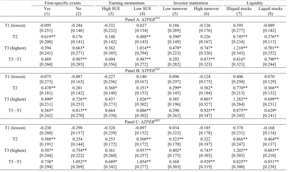
(23) significant at the 1% and 5% level, respectively. The negative exposure to SMB occurs when large firms outperform small firms. Also, the long-short portfolio turns out to be negatively exposed to the momentum factor when its return is below average. The upside exposure to MOM is positive and significant at the 1% level. This indicates that the extra-performance is obtained by timing the exposure to risk factors. Therefore, the strategy avoids the negative payoffs of the momentum and size factors and is mostly neutral to the market. We demonstrate that more weight is given to pro-cyclical (neutral) stocks when the probability of recession is low (high). Finally, we perform several robustness tests. First, it is possible that our results are driven by firmspecific events that occur in concomitance with target price releases. We find that the strategy based on likely valuable target price revisions driven by information discovery yields a positive and significant riskadjusted return, while the strategy based on information interpretation does not. Nevertheless, the risk-adjusted returns of the former and the latter are not statistically different at the usual level. Second, we check whether our results are driven by the post earnings announcement drift (PEAD). We find that it is not the case since the portfolios built on target price revisions of stocks with low (high) standardized unexpected earnings (SUE) earn (no) extra-positive return statistically significant at the 1% level. Third, we investigate whether limited investors’ attention is a plausible explanation for the price drift that drives the extra-performance. We demonstrate that the performance of portfolios constructed with high and low turnover stocks are not statistically different. Fourth, to examine whether the results are driven by illiquid stocks, we sort firms into two groups according to their liquidity. Our results show that portfolios based on likely valuable target price revisions of illiquid stocks do not outperform those based on liquid stocks. Fifth, the remaining question is whether the long-short strategy based on valuable target price revisions resists transaction costs. Our strategy involves a 130% monthly turnover meaning that transaction costs should be lower than 18 bps for the extra-performance to survive. However, it turns out that strategies involving less rebalancing or being more profitable could survive. For instance, a strategy that reduces the turnover by opening every day a one-month long-short position yields significant net-of-fees monthly returns for transaction costs up to 80 bps.. 9.

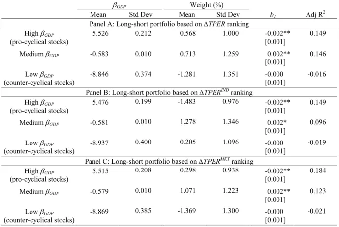
(24) This paper contributes to the literature in several ways. First, we add to the literature on the investment value of financial analysts’ advices by studying the role of target prices. Contrarily to stock recommendations, target prices have been the focus of few studies. We demonstrate that there is not a one-to-one correspondence between target prices and stock recommendations. Closely related to our study, Da and Schaumburg (2011) show that the target price consensus has investment value. We depart from them with respect to both the universe of stocks that we cover and the methodology that we use to derive our results. More importantly, we show that the abnormal risk-adjusted performance originates from the ability of financial analysts to adjust target prices according to the expected probability of recession; i.e., the weight invested in cyclical (neutral) stocks increases when the probability is low (high). Second, we complement previous finding on stock recommendations with target prices. Consistent with Jegadeesh et al. (2004), we find that portfolios based on target prices are tilted toward momentum in good times. However, analysts avoid small and momentum firms and favor value stocks in (expected) bad times. Third, our results show that the rotation strategy from cyclical stocks to neutral stocks drives the positive performance of target prices based portfolios. This finding contradicts Kadan, Madureira, Wang and Zach (2012), who document stock picking ability and no market timing skills. Fourth, we show that target prices can be appropriately filtered ex-ante with the model of Loh and Stulz (2011). However, we find that target prices based on both information discovery and information interpretation are valuable at the one-month horizon. The remainder of the chapter is organized as follows. In the next section, we provide details on the differences between recommendations and target prices which are related to their informational content, the brokers’ rating scales, and the ambiguous translation from the data provider. Section 1.3 describes the construction of target price based portfolios. It also presents how to determine ex-ante target prices that are potentially valuable. Section 1.4 presents the performance of portfolios based on target price revisions. Section 1.5 reports the time-varying exposure of these portfolios to risk factors. Section 1.6 examines potential confounding effects that could also explain portfolios performance. Section 1.7 concludes.. 10.

(25) 1.2. On the informational content of stock recommendations and target prices The target price obtained from a valuation model reflects the information contained in the earnings forecasts as well as additional material information such as the risk of the investment and the cost of capital. Among analysts’ production, stock recommendations are extremely popular. Therefore, it is legitimate to wonder whether the investment value of the target price differs from that of the corresponding recommendation. In the remainder of this section, we discuss how target prices and stock recommendations are connected and what their respective advantages are.. 1.2.1. Target prices and recommendations: Why are they different? The target price is a continuous variable that is translated into the stock recommendation, a categorical variable. The aim of the categorization is to create clusters that investors should consider as similar when making investment decisions. However, this procedure induces a loss of information and creates heterogeneity within clusters. To illustrate this point, consider the following example. On September, 20th, 2011, Carlo Santarelli, a research analyst at Deutsche Bank, issued a “Hold” recommendation for two lodging stocks, Choice Hotel Intl. and Gaylord Entertainment Co.1 However, their upside potential was different, with a target price expected return of 1.5% and 14.3%, respectively. Some brokers assign recommendations subjectively. For example, Deutsche Bank does not include any official threshold that stock expected return has to exceed to receive a “Buy” recommendation. As shown in the example, analysts are free to assign identical (different) recommendations to stocks with different (same) investment prospects. The resulting heterogeneity of stocks receiving the same rating translates into biased and predictable market reactions. Consequently, by equally treating the stocks with the same rating, or recommendation change, researchers do not estimate appropriately the market reaction. In a nutshell, the reactions and the expectations based on recommendations are biased, while the ones based on target prices are not.. 1. The corresponding report is available at http://www.luxesf.com/wp-content/uploads/2011/10/DB-on-lodgingindustry.pdf. 11.

(26) Subjectivity in the assignment of ratings can be interpreted as a positive feature since it allows the analysts to integrate proprietary “soft” information. If this was the case, recommendations would be more informative that target prices. However, empirical evidence shows the opposite; see Brav and Lehavy (2003). In addition, recommendations are strategically biased because, contrary to earnings forecasts and target prices, their accuracy is hardly gauged; see Lin and McNichols (1998). Subjectivity is not limited to recommendations’ rating but also to their definition. In fact, the definitions of the rating scale are brokerage house dependent; see Kadan et al. (2012). Brokers use either an absolute benchmark (e.g., Citigroup), an industry benchmark (e.g., Morgan Stanley), a market benchmark (e.g., UBS), or no explicit benchmark at all (e.g., Deutsche Bank); see Appendix, Table 1.A.1. Therefore, even if equally named, stock recommendations should be interpreted differently. For instance, a “Sell” recommendation from Citigroup means a negative expected return, whereas Raymond James & Associated assigns a “Sell” as soon as the stock is expected to underperform the market. Conversely, recommendations defined similarly can be named differently. For example, the recommendations from Credit Suisse and UBS are defined with respect to a market benchmark but only Credit Suisse uses the appropriate terms “Underperform” and “Outperform”. Moreover, brokerage houses change their rating scales over time, making the comparison of recommendations released at different periods awkward. To be more specific, half of the one hundred most active brokers, representing more than 90% of the stock recommendations, changed their rating scale at least once during the 1990-2011 period. Kadan et al. (2012) suggest that investors and researchers should adjust recommendations appropriately but the differences across brokers and the changes of scale within brokers render this task extremely cumbersome. Since the approval of NASD Rule 2711 in May 2002, the majority of the brokers switched from a fivetier rating system to a three-tier system. Despite that, I/B/E/S still uses a five-tier scale as standard rating system. This may suggest that I/B/E/S recommendations are unambiguous, since the differences that exist across brokerage houses are smoothed by the mapping. However, the mapping is decided by the brokerage houses (not I/B/E/S) and, as a result, the ambiguity remains. Appendix, Table 1.A.1, shows that the I/B/E/S rating is as ambiguous as the brokerage house ratings. For instance, the definition of. 12.

(27) “Overweight” assigned by Morgan Stanley is equivalent to “Outperform” with Wells Fargo. However, the “Outperform” of Wells Fargo is mapped as a “Strong Buy” in I/B/E/S, whereas the “Overweight” of Morgan Stanley translates into a “Buy”.2 This heterogeneity poses a serious challenge to archival research using recommendations because there is no one-to-one relation between the rating scale and the expected performance provided by the broker. To summarize, each broker speaks its own language and the translator (I/B/E/S) does not come up with a reliable translation. Target prices naturally circumvent this ambiguity because, for all brokers and time periods, they represent the expected stock price over a defined and common horizon (mostly twelve-month horizon).. 1.2.2. Empirical evidence To illustrate the differences between recommendations and target prices, we obtain target prices and stock recommendations from the I/B/E/S detail database. We match target prices and recommendations released by the same broker, for the same firm, during the three-day window surrounding the announcement of the target price. This procedure results in 136,982 target prices and recommendations over the 1999-2011 period. The upside (downside) potential is the analyst expected return, which is defined as (TP-P)/P, where TP is the target price and P the closing price on the announcement day. For each standard rating on the I/B/E/S rating scale, Figure 1.1 displays the corresponding kernel-based distribution of the analyst expected return. [Insert Figure 1.1 about here] Figure 1.1 illustrates empirically that brokerage houses indeed use three-tier rating scales and that the I/B/E/S conversion to a five-notch scale is inappropriate and misleading. As a matter of fact, the distributions of the upside potential of stocks rated as “Buy” and “Strong Buy” are very close since 86.0% of the “Buy” recommendations have an upside potential that overlaps with “Strong Buy” recommendations. Similarly, according to the I/B/E/S rating, the expected performance of a “Sell” should. 2. Even more striking, the definition given by Credit Suisse for the “Outperform” recommendations is stricter than the one given by Wells Fargo. Nevertheless, “Outperform” recommendations of Credit Suisse are mapped with “Buy”, i.e. a rating worse than the one received by the looser recommendations of Wells Fargo.. 13.

(28) be lower than that of an “Underperform”. However, the downside potential of 58.4% of the “Sell” recommendations overlaps with “Underperform”. Therefore, not combining “Sell” with “Underperform” recommendations, and “Buy” with “Strong Buy” respectively, overestimates the impact of the extreme ratings. Figure 1 reflects also the heterogeneity of brokers’ rating. For instance, a stock with the upside potential of Gaylord Entertainment (14.3%) has a 66% probability of receiving a “Buy”, 32% of receiving a “Hold”, and 2% of receiving a “Sell”. This happens because there is a significant overlap between the different ratings. When the five-notch rating is merged into a three-notch rating, i.e. “Sell” with “Underperform” and “Buy” with “Strong Buy”, “Hold” recommendations overlap with “Sell” (“Buy”) recommendations 23.1% (36.9%) of the time. There is also a 6% overlap between “Sell” and “Buy” recommendations. To summarize, the above results show that recommendations and target prices do not convey the same information. These differences arise because of three reasons: i) the information lost when target prices are mapped to recommendations, ii) the subjectivity with which brokers define their rating system and iii) the inappropriate mapping of recommendations with the five-tier I/B/E/S rating system. Target prices are not subject to any of these drawbacks. For all these reasons, we argue that target prices are best suited to answer our research question.. 1.3. Construction of target price-based portfolios 1.3.1. Data Target prices and stock prices are obtained from the Institutional Broker Estimate Service (I/B/E/S) and the Center for Research in Security Prices (CRSP) respectively. We rely on the unadjusted version of the databases to avoid the issues related to adjusted data; see Payne and Thomas (2003). We focus on the target prices issued between 1999 and 2011, by identifiable analysts, on US firms.3 Target prices have to meet the following criteria. First, they must have a twelve-month forecast horizon. This restriction affects a small number of observations since 98% of the target prices have a twelve-month horizon. Second, to 3. We identify US firms as the ones having a COMPUSTAT currency code of “USD” and a CRSP share code of 10 or 11; see Daniel, Grinblatt, Titman and Wermers (1997) and Wermers (2004).. 14.

(29) obtain a meaningful comparison between target prices and stock prices, we only retain the target prices expressed in USD. Third, to ensure that firms are of sufficient interest to investors, we focus on firms followed by at least three analysts. Fourth, we require a valid closing share price above one USD on the announcement date. Appendix, Table 1.A.2, Panel A reports the details of the sample selection and the annual statistics. Our selection procedure yields a sample of 735,191 target prices, made by 8,732 analysts (655 brokerage houses), on 6,223 US firms that represent 82.4% of the total market capitalization; see Appendix, Table 1.A.2, Panel B. The number of analysts and firms followed remain roughly constant over time while target prices are issued more frequently at the end of the sample period. The fraction of the market capitalization of our sample decreases over time, but still represents more than 75% of the US stock market capitalization at the end of the sample period. To determine the likelihood of investment value of target prices, we collect additional information from the All-American rankings published yearly by the Institutional Investor magazine. We identify firm-specific events, in addition to I/B/E/S (earnings announcements), from I/B/E/S Guidance (management guidance), SDC (mergers and acquisitions, equity issuance), and LPC Dealscan (syndicated loans). Institutional ownership is computed using data obtained from 13F filings that we download from the EDGAR database. Table 1.1 describes the size, book-to-market, and momentum characteristics of our sample relative to the NYSE universe.4 [Insert Table 1.1 about here] Overall, analysts tend to follow large and growth firms, but there are important changes over time. For instance, we observe an almost parallel trend toward small and value firms. The trend started when small. 4. The tercile breakpoints are constructed using all the NYSE stocks. Each December, we compute the three variables for all the firms in our sample. Size and book-to-market are computed as in Davis, Fama and French (2000), momentum is the buy-and-hold return from the beginning of January till the end of November. The variables are then used to classify the target prices issued in the following year into terciles. We include in the NYSE universe only the stocks with a CRSP share code equal to 10 or 11.. 15.

(30) and value firms were outperforming large and growth firms, respectively, and reverted in 2008 with the financial crisis.5. 1.3.2. Target price interpretation and portfolio construction Previous studies show that stock recommendation revisions are more informative than recommendations themselves; see, e.g., Boni and Womack (2006) and Jegadeesh and Kim (2010). Similarly, Feldman et al. (2012) find larger abnormal market-adjusted returns around the revision of target prices. Therefore, we measure the revision of the expected return embedded in target prices in two steps. First, we compute the target price expected return defined as: (1) TPERi ,b , . TPi ,b , Pi ,. 1 ,. where TPi,b, denotes the twelve-month target price for firm i, issued by broker b at date , and Pi, denotes the closing stock price for firm i at . If the target price is released between 4:30 PM and 11:59 PM, Pi, is replaced by the closing price of the next trading day; see Loh and Stulz (2011). As we retain only target prices with a twelve-month horizon, TPERs represent the annual expected returns. Second, we compute the revision of the expected return to measure the new information conveyed by the target price: (2) TPERi , b ,  TPERi , b ,  TPERi , b , 1 , where  is the date of the previous target price from the same brokerage house b for firm i. TPER is computed only if TPERi,b,-1 is still valid at , i.e. if it meets three conditions: i) the end of the forecast horizon is after , ii) TPi,b,-1 is the most recent target price issued on firm i by the brokerage house b, and iii) broker b did not stop covering firm i from  to . To construct the portfolios we follow Barber et al. (2001). As of the end of day , stocks are assigned to tercile portfolios according to the value of TPERi,b,. The cutoffs of the tercile portfolios are based on. 5. There is no clear preference for high or low momentum stocks. In fact, the proportion of past winners and losers varies strongly over time. 16.

(31) the distribution of valid TPER released during the last three months.6 We use terciles to be consistent with the three-tier recommendation scale. The portfolio consisting of stocks in the highest (lowest) TPER tercile can be interpreted as a “Buy” (“Sell”) portfolio. A stock enters the portfolio at the end of the announcement day and exits the portfolio after a month (21 trading days) or when the broker revises its target price. To avoid cross-correlation problems arising from the inclusion of identical returns, we follow Brav and Lehavy (2003) and keep each stock only once.7 The composition of each portfolio p being known at the date , the value-weighted return for the following trading day, denoted t+1, is computed as in Barber et al. (2001). The return is given by: n p ,. (3). Rp ,t 1   xi ,t Ri ,t 1 , . i 1. . . where Rp ,t 1 ( Ri ,t 1 ) denotes the return of portfolio p (stock i) at t+1, np, the number of stocks in portfolio p at the date , and xi ,t is the weight of stock i, computed as the ratio of the market value of firm i to the aggregated market capitalization of the firms in portfolio p. We employ value-weighted portfolios to avoid an overstatement of returns due to bid-ask bounces; see Blume and Stambaugh (1983) and Canina, Michaely, Thaler and Womack (1998). For each portfolio, the daily returns are then compounded over the nm trading days of the month m to obtain portfolio’s p monthly returns: nm. (4). Rp , m   1  Rp , j   1 . j 1. This procedure yields a time-series of monthly returns for each tercile portfolio which is evaluated with the Carhart (1997) four-factor model.. 6. Results remain unchanged with a six-month window. Longer windows are less well suited because target prices are revised frequently (every three months on average) and market expectations are changing over time. These results as well as other unreported results are available from the authors upon request. 7 The cross-correlation problem arises when a stock is selected by several brokers during the holding period. If these multiple entries are considered as different holdings of the portfolio, the correlation between the components of the portfolio increases, as well as the volatility of the whole portfolio. A stock can appear in several distinct portfolios simultaneously. Note that the standard event study methodology does not exclude these stocks either; see, e.g., Womack (1996), Altınkılıç and Hansen (2009), Jegadeesh and Kim (2010), and Loh and Stulz (2011).. 17.

(32) We consider two additional measures of the information content of target prices. First, there is evidence that analysts’ production is more valuable if considered at the industry level. For instance, Boni and Womack (2006) show that recommendations have more investment value when they are considered within industries. Similarly, Da and Schaumburg (2011) find that rankings of TPERs are more informative within industries. For this reason, we also construct portfolios according to the industry-adjusted revision of TPER, defined as: (5) TPERiIND  TPERi ,b ,  TPER ind ( i ), , , b , where TPERind (i ), is the average valid TPER of firms operating in the same industry as firm i. We compute the average excluding firm i to prevent spurious correlations between TPER ind ( i ), and TPERi,b, in industries with few firms. We use the 68 GICS industries (6 digits) classification because it matches analysts’ industry specialization; see Boni and Womack (2006). We interpret TPERIND as the revision of the industry-adjusted expected return. We also compute the expected return in excess to the market expected return. In fact, Kadan et al. (2012) show that analysts often issue recommendations based on a market benchmark. Therefore, we construct portfolios according to a variable that measures the revision of the market-adjusted expected return, defined as: (6) TPERiMKT  TPERi ,b ,  TPER , , b , where TPER  is the average of valid TPERs. To construct portfolios according to TPERIND and TPERMKT, we obtain the cutoffs of the tercile portfolios from the distributions of valid TPERIND and TPERMKT, respectively, and we use the methodology described previously. Table 1.2 reports the descriptive statistics of 595,995 target price revisions. The average and median TPER is 0% with a significant variability both between and within years. For instance, the annual average ranges from -4.5% (2009) to 5.0% (2000). The dynamics of TPER shows that analysts’ forecasts are stickier than market prices and that the analysts revise their target prices with a delay compared to the market. In fact, TPER are inversely related to stock market returns, i.e. they are higher when market returns are negative (2000, 2008) and lower when market returns are positive (2003, 2009). The 18.

(33) interquartile range varies between 13.5% and 28.5%, showing that there is a large cross-sectional dispersion of TPER across stocks. Interestingly, the largest interquartile ranges coincide with the years of downturn. The descriptive statistics of TPERIND and TPERMKT are similar to the ones of TPER. TPERIND can be computed only for 594,383 target price announcements because some firms are not assigned to any valid industry or because there are too few observations to compute TPER ind ( i ), . The signals used to construct the portfolios are economically significant; see Appendix, Table 1.A.3. For instance, the average of TPER is -21.4% (21.5%) in the first (third) tercile portfolio. Similar numbers are obtained for portfolios based on TPERIND and TPERMKT. [Insert Table 1.2 about here]. 1.3.3. Likely valuable target prices Given the high number of target prices released (i.e., 230 target prices per day on average), we determine ex-ante with a model, which ones are potentially valuable and analyze whether this filter improves the performance of the tercile portfolios. We estimate the parameters of the model as follows. First, we define a dummy variable, Valuable, that equals 1 if the target price is valuable ex-post and 0 otherwise. A target price is considered to be valuable if the TPER revision is positive (negative) and the corresponding cumulated abnormal return over the holding period is statistically positive (negative) at the 5% level; see Loh and Stulz (2011).8 We focus on the cumulated abnormal return in the month (21 trading days) that follows the announcement of the target price. The benchmark is the Carhart (1997) four-factor model. The parameters of the four-factor model are estimated running a daily time-series regression over the estimation window [-150; -1], where day zero is the date at which the target price is announced. To properly identify the factor-exposures and compute the abnormal returns, we require stocks to have at least 120 observations over the estimation window and valid closing prices on the event-day zero and 21.. 8. The results are similar when TPERIND or TPERMKT are used to identify likely valuable target prices. In fact, for more than 91% of TPER, TPERIND, and TPERMKT have the same sign.. 19.

(34) The factor-exposures and the abnormal returns are estimated using the dummy variable approach of Salinger (1992).9 Second, when at least a target price is released on trading day, we identify the target prices released during the last three months skipping the most recent twenty-one trading days. We skip this period because a target price is known to be valuable only after this period. As we aim at predicting ex-ante whether a target price is likely valuable, we estimate Probit regressions that relate the dependent variable Valuable to the analyst, firm, and target price characteristics as defined in Loh and Stulz (2011). The list and the definition of the explanatory variables are presented in Appendix, Table 1.A.4. As the determinants of valuable target prices can change with the direction of the revision, we separate target price revisions according to their sign and fit two Probit models: one for positive and one for negative TPER. We use the estimated coefficients to predict the likelihood that a target prices released on trading day  is valuable. These predicted probabilities are compared to the median fitted probability to separate the most likely valuable from least likely valuable target prices. In the remainder of the paper we refer to them as likely valuable and unlikely valuable, respectively. Notice that all the variables are known ex-ante (i.e. before date ) so that the prediction is made out-of-sample and it can be implemented in real time. Having determined likely valuable target prices, we construct portfolios using the methodology detailed previously. We obtain two sets of tercile portfolios, each containing either likely valuable or unlikely valuable target prices.. 1.4. Performance of portfolios 1.4.1. Unconditional portfolios In this section, we discuss the performance of the portfolios that consider the whole sample of target prices. To investigate the speed at which the information is incorporated into prices, we implement the strategy using different starting dates. We focus on strategies with a one-month holding period that start 9. To account for potential missing returns in the estimation window, we run a WLS regression with observations weighted by the inverse of the square root of the number of trading days between two valid returns; see Heinkel and Kraus (1988).. 20.

(35) either at the end of the announcement day ([+1 ; +21]) or at the beginning of the following two months ([+22 ; +42] and [+43 ; +63], respectively). To verify that the information is not incorporated into prices in the days that immediately follow the announcement, we also compute the monthly return of a strategy that starts investing in a stock five days after the target price release ([+5 ; +21]). Table 1.3 reports both the raw and the risk-adjusted returns of the tercile portfolios for the four holding periods.10 [Insert Table 1.3 and Figure 1.2 about here] Table 1.3, Panel A, reports the raw returns of the portfolios based on TPER. The strategy starting at the announcement date that buys high TPER stocks and sells low TPER stocks earns an average 0.44% per month (statistically significant at the 1% level). The price trend is significant and is not concentrated in the few days after the announcement since the [+5; +21] portfolios show that the returns are statistically significant at the 5% level. In Figure 1.2, Panel A, we see that the gap between abnormal returns of the top and bottom portfolios continues to increase over the whole period considered, even if the trend is more pronounced during the first month after the target price announcement. In fact, the economically small returns (below 10bps), and statistically insignificant at the 5% level, of the [+22; +42] and [+43; +63] portfolios demonstrate that this trend is not significant beyond the first month. The results obtained for TPERIND are similar, the statistical significance being slightly lower. For instance, the risk-adjusted performance of the portfolio based on industry-adjusted target price revisions that start investing five days after the target price release and stops at the end of the month ([+5; +21]) is no longer statistically significant at the 5% level (p-value = 9% for the raw return). Figure 1.2, Panel B, shows that the dynamics of TPERIND portfolio returns is less clear cut than the one of TPER portfolios. The top portfolio grows at a lower rate, while the bottom portfolio, after a rapid adjustment in the first ten trading days following the announcement, displays a small reversal. The performance of the portfolios obtained with a ranking based on TPERMKT is similar to the one obtained for TPER and confirms that the post target price announcement drift lasts beyond the first days following the announcement.. 10. Standard errors are corrected for heteroskedasticity and autocorrelation using the Newey and West (1987) estimator with six lags. The results do not change qualitatively with twelve lags.. 21.

(36) The results for risk-adjusted returns are presented in Table 1.3, Panel B. We observe marginal changes. The long-short strategy initiated at the announcement date earns positive risk-adjusted returns (0.49% per month). Overall, the results indicate that the information contained in expected return revisions is incorporated within the month following the announcement of the target price but is not limited to the first days after the announcement. For this reason, the focus of the rest of the paper is on the performance of these first-month portfolios.11. 1.4.2. Portfolios performance of likely valuable target prices We now turn to the portfolios constructed with likely valuable target prices. Out of the 593,872 target prices for which the information is available, 26.3% are valuable. The sample of valuable target prices is slightly tilted toward observations with positive TPER since 53% of valuable observations have a positive revision of implied expected returns. Table 1.4, Panel A, reports the risk-adjusted performance of the two sets of portfolios. As expected, the extra-performance of long-short portfolios is limited to the portfolios constructed with likely valuable target prices. The risk-adjusted performance is economically large and statistically significant at the 1% level for target price revisions (0.81% per month) as well as for the industry (0.66% per month) and the market (0.87% per month) adjusted target price revisions. The over-performance of the likely valuable portfolios comes exclusively from the long leg. Figure 1.3 also illustrates that the high TPER portfolio shows a clear upward trend over the whole period, whereas the low TPER portfolio reacts sharply in the few days following the announcement, and then exhibit a reversal. The rightmost columns of Table 1.4 contain the performance of the portfolios constructed with unlikely valuable target prices. Regardless of the interpretation of target prices, the performance of portfolio T3 and T1 is never statistically significant at the usual critical levels. Figure 1.3, illustrates that the abnormal performance of unlikely valuable portfolios do not show any drift. [Insert Table 1.4 and Figure 1.3 about here] 11. Similar portfolios constructed on TPER (implied return instead of revision of implied return) generate abnormal returns up to four trading days. Beyond this horizon, no abnormal return is observed.. 22.

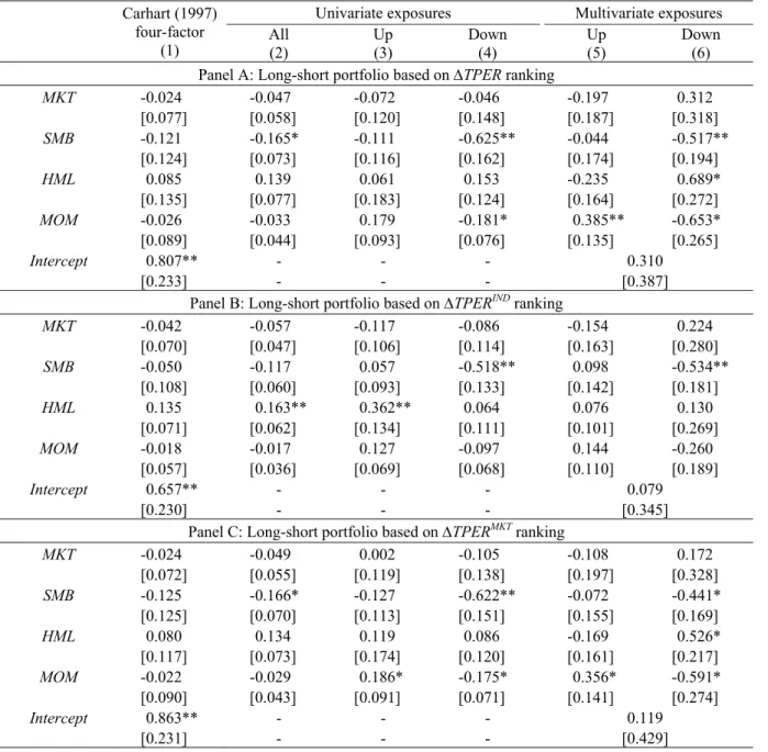
(37) To verify the robustness of our filtering procedure (identification of likely valuable target prices), we run an OLS regression where the dependent variable is the ratio of the cumulated abnormal returns over the holding period divided by the corresponding standard error (t-stat associated to the one-month CAR), the independent variables being the ones of the Probit model. Table 1.4, Panel B, shows that our results are robust to the methodology.12 However, a target price can simply be a false positive, i.e. the target price is classified as valuable when it is not. To gauge the impact of the Type I error, we determine whether a target price is valuable with a test whose critical value is based on the Gumbel distribution; see Boudt, Croux and Laurent (2011). This procedure strongly decreases the probability of having false discoveries. Table 1.4, Panel C, shows that portfolio performance is only marginally affected by false discoveries.. 1.5. Time-varying risk exposures The long-short strategy based on TPER being dynamic, the exposure to the factors potentially varies with market and economic conditions. In this section, we analyze the risk exposures of our strategy conditionally on the market movements.. 1.5.1. Upside and downside risk Risk adverse investors care differently about losses and gains. Therefore, investors ask a larger risk premium to hold assets that co-vary strongly with the market during market declines. Ang, Chen and Xing (2006) show that stocks with downside exposure have higher average returns. They also quantify the downside risk premium at approximately 6% per year. Lettau, Maggiori and Weber (2014) find further evidence supporting the existence of a downside risk premium for other asset classes like options, commodities, and currencies. To verify whether the abnormal performance of portfolios based on target prices is attributable to downside risk exposure, we follow Ang et al. (2006) and estimate the upside and downside market betas of our strategies. In addition, we also include conditional exposures to size, value,. 12. We also build portfolios based on target prices that are likely valuable with both the Probit and the t-statistic regression. The results are similar.. 23.