Publisher’s version / Version de l'éditeur:
Building and Environment, 39, April 4, pp. 421-431, 2004-04-01
READ THESE TERMS AND CONDITIONS CAREFULLY BEFORE USING THIS WEBSITE.
https://nrc-publications.canada.ca/eng/copyright
Vous avez des questions? Nous pouvons vous aider. Pour communiquer directement avec un auteur, consultez la première page de la revue dans laquelle son article a été publié afin de trouver ses coordonnées. Si vous n’arrivez pas à les repérer, communiquez avec nous à [email protected].
Questions? Contact the NRC Publications Archive team at
[email protected]. If you wish to email the authors directly, please see the first page of the publication for their contact information.
NRC Publications Archive
Archives des publications du CNRC
This publication could be one of several versions: author’s original, accepted manuscript or the publisher’s version. / La version de cette publication peut être l’une des suivantes : la version prépublication de l’auteur, la version acceptée du manuscrit ou la version de l’éditeur.
For the publisher’s version, please access the DOI link below./ Pour consulter la version de l’éditeur, utilisez le lien DOI ci-dessous.
https://doi.org/10.1016/j.buildenv.2003.09.016
Access and use of this website and the material on it are subject to the Terms and Conditions set forth at
Development of a radiant heating and cooling model for building
energy simulation software
Laouadi, A.
https://publications-cnrc.canada.ca/fra/droits
L’accès à ce site Web et l’utilisation de son contenu sont assujettis aux conditions présentées dans le site LISEZ CES CONDITIONS ATTENTIVEMENT AVANT D’UTILISER CE SITE WEB.
NRC Publications Record / Notice d'Archives des publications de CNRC:
https://nrc-publications.canada.ca/eng/view/object/?id=48a7bba2-1464-4125-bcdb-3d24e39bf8b7 https://publications-cnrc.canada.ca/fra/voir/objet/?id=48a7bba2-1464-4125-bcdb-3d24e39bf8b7Development of a radiant heating and cooling model
for building energy simulation software
Laouadi, A.
NRCC-46099
A version of this document is published in / Une version de ce document se trouve dans :
Building and Environment, v. 39, no. 4, April 2004, pp. 421-431
DEVELOPMENT OF A RADIANT HEATING AND COOLING MODEL
FOR BUILDING ENERGY SIMULATION SOFTWARE
Abdelaziz Laouadi
Indoor Environment Research Program, Institute for Research in Construction, National Research Council Canada,
1200 Montreal Road Campus, Ottawa, Ontario, Canada, K1A 0R6 Tel.: (613) 990 6868
Fax: (613) 954 3733
ABSTRACT
Efficient radiant heating and cooling systems are promising technologies in slashing energy bills and improving occupant thermal comfort in buildings with low energy demands such as houses and residential buildings. However, the thermal performance of radiant systems in buildings has not been fully understood and accounted for in currently available building energy simulation software. The challenging tasks to improve the applicability of radiant systems are the development of an accurate prediction model and its integration in the energy simulation software. This paper addresses the development of a semi-analytical model for radiant heating and cooling systems for integration in energy simulation software that use the one-dimensional numerical modeling to calculate the heat transfer within the building construction assemblies. The model combines the one-dimensional numerical model of the energy simulation software with a two-dimensional analytical model. The advantage of this model over the one-dimensional one is that it accurately predict the contact surface temperature of the circuit-tubing and the adjacent medium, required to compute the boiler/chiller power, and the minimum and maximum ceiling/floor temperatures, required for moisture condensation (ceiling cooling systems), thermal comfort (heating floor systems) and controls. The model predictions for slab-on-grade heating systems compared very well with the results from a full two-dimensional numerical model.
INTRODUCTION
The use of radiant heating/cooling systems in houses has been growing in recent years. In Europe, for example, the use of radiant heating/cooling technique represents more than 50% in newly constructed houses [1-2]. The intent of radiant systems is to lower thermostat set point temperature in winter and to increase it in summer, resulting in a substantial energy savings for heating and cooling as compared with conventional systems. The energy savings from radiant heating/cooling may reach more than 30%, as demonstrated in some theoretical/experimental case studies [3-5]. However, these energy savings may not be achieved without an accurate prediction model, an appropriate control strategy and a careful design. The prediction model integrated within a building energy simulation program will aid building and system designers to specify and size energy-efficient radiant systems and to improve indoor thermal comfort
PROBLEM
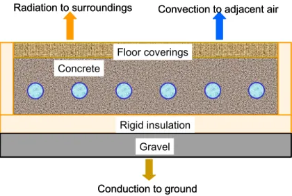
Radiant heating and cooling systems are very complex systems since they involve different heat transfer mechanisms –conduction within the slab, radiation between the radiant surface and the surrounding surfaces, convection between the radiant surface and the adjacent zone air, and conduction between the slab and the ground. Integration of a radiant heating/cooling model into a building energy simulation program introduces another complexity to the modeling process of radiant systems. The radiant system has to interact with the operation of the building control system to ensure indoor thermal comfort and avoid overheating in winter and overcooling in summer. The prediction model, therefore, has to take into account the transient nature of the radiant system and the dynamic controls. The prediction model should adequately predict heat transfer from the slab to the surrounding space whether the control is ON or OFF. Radiant systems are multi-dimensional by nature. Energy simulation software that use the
one-dimensional numerical modeling to compute heat flows within building structures over-predict the thermal capacity of the radiant system, and therefore result in over-sizing the radiant system with the added cost. Furthermore, such software cannot predict the cold and hot spots of the floor or ceiling surface, which may cause thermal discomfort, ceiling moisture condensation, and the moisture-related damage to the radiant surface (and repair expenses).
PREVIOUS WORKS
Extensive studies have been devoted to laboratory testing of radiant systems with the main aim to quantify the thermal performance and response of radiant systems upon using conventional or newly developed control strategies [6-11]. However, from the modeling point of view, there are a few analytical studies for the prediction of thermal performance of radiant systems. Earliest models by Kollmar and Liese [12] assumed that the slab operates as a plate fin and loses heat from its upper surface. Leal and Miller [13] used an analytical-numerical method to solve the
temperature within pavement heating installations. Zhang and Pate [14-15] developed a two-dimensional finite-difference method for ceiling panels, which then was used to develop a simplified model for radiant slab heating. Athienitis [16] developed a one-dimensional finite-difference method for floor radiant heating. Kilkis et al. [17] developed a steady-state, composite-fin model to design radiant heating and cooling systems. Kilkis and Sapci [18] and Kilkis and Coley [19] subsequently used their composite-fin model to develop software for the design of floor and sub-floor heating and cooling systems.
Integration of radiant heating and cooling models into building energy and thermal analysis software has been very limited. The ESP-r program uses the one-dimensional transient
numerical modeling and a node heat injection/extraction method to model radiant heating/cooling systems. Maloney et al. [20] developed a radiant heater model for the BLAST program. Strand and Pederson [21-22] used a conduction transfer function method to develop a radiant heating and cooling model for the EnergyPLus program. Stetiu et al. [23] developed a detailed model for cooling radiant systems for the RADCOOL software that works under the SPARK environment. Some artifices have also been employed to model radiant heating systems. Chun et al. [24] used the SERI-RES program and modeled radiant slab heating as a fictitious zone that provides heat to the conditioned zone. Miriel et al. [25] used the TRNSYS program to model a ceiling radiant panel heating and cooling system.
It should be noted that the steady-state simplified models cannot be used for transient systems and are not valid when the control system is not operating. Furthermore, the one-dimensional transient models under-predict the circuit water temperature, and therefore over-predict the heating/cooling capacity of the boiler/chiller.
OBJECTIVES
The specific objectives of this paper are:
To develop a two-dimensional prediction model for radiant systems for integration in energy simulation software that use the one-dimensional numerical modeling; and
To validate the developed model using the numerical modeling approach.
MATHEMATICAL FORMULATION
Radiant heating/cooling systems consist of tubes or resistance heating elements embedded in a concrete slab or attached to a radiant surface. The tubes can be laid out within the medium with different patterns. Tubing patterns introduce additional complexity on the prediction of heat exchanges. Two of the most used tubing patterns are serpentine and spiral. In the serpentine pattern, heat transfer is mostly transversal (perpendicular to the tubing plane) while in the spiral
pattern the heat transfer is radial. A typical radiant system may also consist of several circuits serving different surface areas.
Figure 1 shows a typical slab-on-grade heating system. For simplicity purposes, the serpentine pattern is considered in this study although the results apply to both patterns. Figure 2 shows a typical circuit serpentine pattern. The average length of all circuits is noted Lc, and the tubes
outside and inside diameters are noted as Do and Di, respectively. The tubes are uniformly
spaced with a distance w. The transport fluid enters a given circuit with an inlet temperature Tin,
and exists with an outlet temperature Tout. Owing to this temperature difference, heat transfer
takes place between the transport fluid and the adjacent medium.
ASSUMPTIONS
The following assumptions are used in the mathematical modeling:
• The temperature gradients along tubing (z-axis) are neglected compared to those in the perpendicular plane. This assumption holds when the ratio of the tubing spacing to circuit length is very small (w/Lc << 1). In this regard, the outside surface temperature of tubing can
be considered as uniform.
• The radiant system edges are adiabatic (well insulated).
• Temperature gradients within the tubing material are negligible. This assumption holds when the tubing thickness is very small compared to the interior diameter (Do/Di≈ 1).
HEAT TRANSFER WITHIN THE RADIANT SYSTEM
Since the radiant system configuration exhibits symmetry between tubing circuit passes, only half of the symmetry domain as shown in Figure 3 is considered for the mathematical modeling. The circuit tubing is considered as heat generation sources occurring in a finite volume of the medium. The temperature of the heat source is therefore equal to the temperature of the tubing-medium contact surface. Taking into account the previous assumptions, the heat transfer in the medium is governed by the following fundamental equation:
q
y
T
k
y
x
T
k
x
t
T
c
+
∂
∂
∂
∂
+
∂
∂
∂
∂
=
∂
∂
⋅
ρ
(1) where:c : material specific thermal capacity (J/kg⋅°C); k : material thermal conductivity (W/m⋅°C);
q : heat generation rate per unit material volume (W/m3); T : local temperature (°C) ; and
ρ : material density (kg/m3).
The heat generation rate, which occurs in the volume occupied by the tubing is given by the following expression:
∆
≤
≤
+
∆
≤
≤
∆
=
elsewhere
:
0
y
y
0
and
x,
x
x
x
-x
:
)
t
(
q
)
t
,
y
,
x
(
q
0 q q (2) where:q0 : the heat injection/extraction rate per unit volume (W/m 3
). xq : x-coordinate of the tube’s center point.
∆x, ∆y : designates the dimensions of the heat generation volume.
Considering the heat generation occurs within the volume occupied by the pipe, one obtains the following relation:
4
/
D
y
x
=
∆
=
π
⋅
o∆
(3)The average heat transfer rate per circuit (Qc) injected in or extracted from the medium is
calculated as follows:
0 c c
4
(
x
y
L
)
q
Q
=
⋅
∆
⋅
∆
⋅
⋅
(4)The total heat transfer rate (Qtot) injected in the medium from all circuits is expressed as follows:
c c tot
Q
N
Q
=
⋅
(5)where Nc is the number of circuits.
The number of circuits is calculated based on the radiant surface area as follows:
)
L
w
/(
A
N
c=
rad⋅
c (6)where Arad is the area of the radiant surface.
Equation (1) is subject to different boundary conditions. At the radiant surface (x=0), the surface exchanges heat with the indoor environment via radiation and convection. The surface
temperature may therefore fluctuate from one point to another. The realistic way to describe this boundary condition is to assume that the heat transfer rate is uniform over the radiant surface, since the uniform temperature does not hold. The uniform heat transfer rate is consistent with the fact that the convection and radiation heat transfer coefficients are calculated/correlated based on the average surface temperature, and that the local values of the convection
coefficients are not available in any form of relationship. The boundary condition at the insulated surface (x = s) may be adiabatic, or with uniform temperature if it is in contact with the ground. In practice, the adiabatic condition may not hold. For this reason, a uniform temperature may
represent the realistic condition since the ground temperature is uniform at a relatively deep depth. Finally, the symmetry condition holds across the tubes (y = 0) and at the mid-distance between them (y = w/2). These conditions are expressed as follows:
(
s air c rh
T
T
q
x
T
k
:
0
x
=
+
−
∂
∂
−
=
)
(7))
t
(
T
T
:
s
x
=
=
g (8)0
y
T
:
2
/
w
,
0
y
=
∂
∂
=
(9) where:hc : indoor convection heat transfer coefficient (W/m2°C);
qr : radiation heat transfer density from the radiant surface to the surrounding surfaces
(W/m2);
Tair : indoor air temperature (°C);
Tg : ground temperature (°C) at x = s; and
Ts : surface average temperature (°C) at x = 0.
The radiation heat transfer may be accurately calculated using the view factor method. A linearized form of the radiation heat transfer may also be used as follows:
(
s mrt)
r rh
T
T
q
=
−
(10)(
)
(
s mrt 2 mrt 2 s s rT
T
T
T
h
=
σε
+
⋅
+
)
(11) where:hr : radiation heat transfer coefficient (W/m2°C);
Tmrt : mean radiant temperature of the surrounding surfaces (°C);
εs : radiant surface emissivity; and
σ : radiation constant.
Equation (1) is difficult to solve analytically. A two-dimensional numerical method should be employed to solve for the temperature within the medium. An alternative method is proposed. The alternative method uses a one-dimensional numerical method to solve for the y-averaged temperature within the medium and an analytical solution is appended to the average values. The method is described as follows:
)
t
,
x
(
q
x
T
k
x
t
T
c
+
∂
∂
∂
∂
=
∂
∂
ρ
(12)Where the y-averaged temperature and heat generation rate are given as follows:
∫
⋅
=
w/2 0dy
)
t
,
y
,
x
(
T
w
2
)
t
,
x
(
T
(13)∫
⋅
=
w/2 0dy
)
t
,
y
,
x
(
q
w
2
)
t
,
x
(
q
(14)Taking into account equation (2), equation (14) reduces to the following:
∆
−
∆
≤
≤
+
∆
=
elsewhere
:
0
x
x
x
x
x
:
)
t
(
q
w
y
2
)
t
,
x
(
q
0 q q (15)Equation (12) is subject to the following boundary conditions:
(
s mrt) (
c s air rT
T
h
T
T
h
x
T
k
:
0
x
=
−
+
−
∂
∂
−
=
)
(16))
t
(
T
T
:
s
x
=
=
g (17)Consider that the local temperature may be expressed as the summation of a mean valueT and a perturbation Φ as follows:
)
t
,
y
,
x
(
)
t
,
x
(
T
)
t
,
y
,
x
(
T
=
+
Φ
(18)where the function Φ is to be determined. Φ must satisfy the following condition:
0
dy
2 / w 0=
⋅
Φ
∫
(19)Substituting equation (18) in equation (1) and talking into account equation (12), one obtains the following equation:
q
q
y
k
y
x
k
x
t
c
+
−
∂
Φ
∂
∂
∂
+
∂
Φ
∂
∂
∂
=
∂
Φ
∂
⋅
ρ
(20)Equation (20) is subject to the following boundary conditions:
0
x
:
0
x
=
∂
Φ
∂
=
(21)0
:
s
x
=
Φ
=
(22)0
y
:
2
/
w
,
0
y
=
∂
Φ
∂
=
(23)Introducing the Kirchhoff transformation variables as follows:
y
k
y
;
x
k
x
∂
Φ
∂
=
∂
Ψ
∂
∂
Φ
∂
=
∂
Ψ
∂
(24) one obtains the following equations:q
q
y
x
t
c
2 2 2 2−
+
∂
Ψ
∂
+
∂
Ψ
∂
=
∂
Φ
∂
⋅
ρ
(25)Equation (25) is subject to the following boundary conditions:
0
x
:
0
x
=
∂
Ψ
∂
=
(26)0
:
s
x
=
Ψ
=
(27)0
y
:
w/2
0,
y
=
∂
Ψ
∂
=
(28)Equation (25) may have an analytical solution if the function Ψ consists of a series of a product of separable functions. The function Ψ may be separable if the local thermal capacity (ρ⋅c) and conductivity (k) are constant throughout the calculation domain, which is not the case for radiant systems. An attempt, however, is made to come up with an approximate solution by replacing the thermal capacity (ρc) by its average value over the medium.
Consider that the function Ψ may consist of separable functions as follows:
)
(
)
(
)
(
)
,
,
(
x
y
t
=
F
t
⋅
G
x
⋅
H
y
Ψ
(29)where F(t), G(x) and H(y) are functions to be determined. The space functions G(x) and H(y) should satisfy the heat balance equation at the transient and steady-state regimes. Substituting equation (29) in equation (25) at the steady-state regime, one obtains the following equation:
0 2 2 2 2
q
q
dx
H
d
H
1
dx
G
d
G
1
Ψ
−
=
+
(30)where Ψ0 is the value of Ψ at the steady-state regime. The function Ψ0 is separable if the
following condition holds:
0
C
q
q
−
=
⋅
Ψ
(31)where C is a constant different than zero. The task is now to determine this constant. Taking into account equation (31), equation (30) leads to two equations as follows:
0
A
with
,
0
G
A
dx
G
d
2 2≠
=
⋅
+
(32)0
B
with
,
0
H
B
dy
H
d
2 2≠
=
⋅
+
(33)where A and B are constants to be determined. The constant C is then given by the following equation:
B
A
C
=
+
(34)The functions F, G and H satisfy the following initial and boundary conditions:
0
F
:
0
t
=
=
(35)0
dx
dG
:
0
x
=
=
(36)0
G
:
s
x
=
=
(37)0
y
d
dH
:
2
/
w
,
0
y
=
=
(38)The possible solutions of equations (32) and (33) are expressed as follows:
A
th
wi
),
x
sin(
b
)
x
cos(
a
)
x
(
G
=
⋅
ω
⋅
+
⋅
ω
⋅
ω
=
(39)B
th
wi
),
y
sin(
b
)
y
cos(
a
)
y
(
H
=
′
ω′
⋅
+
′
ω′
⋅
ω′
=
(40)where a, b , a′ and b′ are constants to be determined. Applying the boundary conditions in equations (36) - (38), one obtains the following equations:
0
b
b
=
′
=
(41)n
...,
1,2,
,
0
i
),
s
2
/(
)
i
2
1
(
+
π
=
=
ω
(42)m
...,
1,2,
j
,
w
/
j
2
π
=
=
ω′
(43)The general solution at the steady-state regime then consists of a superposition of the individual solutions, expressed as follows:
∑∑
= =⋅
ω′
⋅
⋅
ω
⋅
⋅
=
Ψ
n 0 i m 1 j j i ij 0 0F
a
cos(
x
)
cos(
y
)
(44)Where F0 is the value of F at the steady-state regime.
Equation (44) is a Fourier series expansion of the function Ψ0. Taking into account equation (31),
(
)
(
)
s
w
/
8
dx
dy
)
y
cos(
)
x
cos(
F
/
q
q
a
2 j 2 i s 0 2 / w 0 j i 0 ijω
+
ω′
⋅
⋅
⋅
⋅
ω′
⋅
ω
⋅
−
=
∫ ∫
(45)Since the coefficients aij are time-independent, one deduces the following relation: 0
0
q
F
=
(46)Performing the integration in equation (45), one obtains the following relation:
(
)
(
)
(
2)
j 2 i j i q i i j ij16
/
s
w
x
cos
x
sin
)
y
sin(
a
ω′
+
ω
⋅
ω′
ω
⋅
⋅
⋅
ω
⋅
∆
⋅
ω
⋅
∆
⋅
ω′
=
(47)The original function Φ may also be expressed as a Fourier’s series expansion as follows:
∑∑
= =⋅
ω′
⋅
⋅
ω
⋅
⋅
=
Φ
n 0 i m 1 j j i ijcos(
x
)
cos(
y
)
b
F
)
t
,
y
,
x
(
(48)Taking into account equation (44) and the feature of Fourier’s series, one obtains the following relation between the coefficients aij and bij
dx
)
x
cos(
d
)
sin(
)
(
k
s
2
)
(
b
a
i 0 k s 0 x s k k kj ij
⋅
ω
⋅
⋅
ξ
⋅
ξ
⋅
ω
⋅
ξ
⋅
ω
−
⋅
=
∑
∞∫ ∫
= (49)Equation (49) may be reduced to:
∑
∞∫
=⋅
⋅
ω
⋅
⋅
ω
⋅
ξ
⋅
=
0 k s 0 i k m kj ijk
(
)
cos
n
(
x
)
cos(
x
)
dx
s
2
b
a
(50)where the value ξm may vary in the interval [s, x]. Equation (50) can be further reduced to the
following:
∫
⋅
≈
=
s 0 ij ijk
(
x
)
dx
s
1
k
b
/
a
(51)From the transient equation (25), one obtains the following differential equation for the function F(t):
(
)
(
F
q
)
0
c
k
dt
dF
0 2 j 2 i+
ω′
⋅
−
=
ω
ρ
+
(52)Equation (52) cannot be solved analytically unless the function of the heat injection rate (q0) is
known a priori. The heat injection rate is usually determined by the thermal control system. The function F should, therefore, be solved using a numerical model. Using the fully-implicit scheme for differentiation, one obtains the following relation to predict the current values of the function F based on the values at the previous time:
(
)
(
)
k
/
c
t
1
q
c
/
k
t
F
F
2 j 2 i 0 2 j 2 i oldρ
⋅
ω′
+
ω
⋅
∆
+
⋅
ρ
⋅
ω′
+
ω
⋅
∆
+
=
(53)where the exponent “old” designates the values at the previous time. The temperature distribution within the medium is then given by:
(
)
∑∑
= =⋅
ω′
⋅
⋅
ω
⋅
⋅
+
=
n 0 i m 1 j j i ij ij(
t
)
/
k
a
cos
x
cos(
y
)
F
)
t
,
x
(
T
)
t
,
y
,
x
(
T
(54)HEAT TRANSFER FROM TUBING CIRCUITS TO ADJACENT MEDIUM
Consider the general case where the adjacent medium to circuit tubing can be solid (e.g., concrete slab), or air space (e.g., sub-floor heating where tubing is emerged in an air space and attached to a surface). When the adjacent medium is solid, the heat transfer from the circuit tubing to the adjacent medium is by conduction. The perfect contact is assumed between the tubing outer surface and the medium (zero contact resistance). However, when the adjacent medium is an air space, heat transfer is more complex, where all the three modes of heat transfer -radiation, convection and conduction- occur at the same time. While the explicit modeling of this system is not attempted here, one would treat the air space as a solid medium with an equivalent thermal conductivity, pre-calculated based on some experimental correlations.
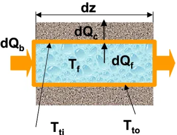
Consider the heat balance around a control volume as shown in Figure 4. Assuming that the tubing thickness is very small compared to the interior diameter, one obtains the following equations:
( )
dt
dT
dz
cA
dQ
dQ
f f f b=
+
ρ
⋅
⋅
(55)( )
dt
dT
dz
cA
dQ
dQ
to t c f=
+
ρ
⋅
⋅
(56) where:Af : fluid cross-sectional surface area (m 2
). At : tubing wall cross-sectional surface area (m
2
). cf : specific heat capacity of fluid (J/kg
o
C). ct : specific heat capacity of tubing material (J/kg
o
C). Qb : heat transfer rate from boiler to fluid per circuit (W).
Qc : heat transfer rate from circuit tubing to adjacent medium (W).
Tto : temperature of outer tubing surface (°C).
Tf : fluid bulk temperature (°C).
ρf : fluid mass density (kg/m 3
).
ρt : mass density of tubing material (kg/m 3
).
The cross-sectional areas of fluid and tubing wall are expressed as follows:
4
/
)
D
D
(
A
;
4
/
D
A
f=
π
i2 t=
π
o2−
2i (57) The heat transfer rates, dQb, dQf, and dQc, are expressed as follows:dz
dT
c
m
dz
dQ
f f b=
−
⋅
(58)(
ti to)
c cT
T
/
R
dz
dQ
−
=
(59)(
f ti)
i fT
T
/
R
dz
dQ
−
=
(60) where:m : circuit fluid mass flow rate (kg/s);
Rc : conductive thermal resistance per unit circuit length (m°C /W);
Ri : convective thermal resistance per unit circuit length (m°C /W); and
Tti : temperature of inner tubing surface (°C).
The conductive and convective thermal resistances are given by:
(
)
t i o ck
2
D
/
D
Ln
R
π
=
(61) f i ih
D
1
R
π
=
(62) where:hf : convective film coefficient at the inner tubing surface (W/m 2
°C); and kt : tube thermal conductivity (W/ m °C).
( )
−
−
⋅
ρ
⋅
⋅
=
dt
dT
cA
R
)
T
T
(
UP
dz
dQ
to t i to f c (63) where:U : overall heat conductance (W/m2°C).
P : perimeter of the pipe cross-sectional surface (m). The product UP is given by the following equation:
)
k
2
/(
)
D
/
D
(
Ln
)
h
D
/(
1
R
R
1
UP
t i o f i c i+
π
=
+
=
(64)Summing up equations (55) and (56) and substituting equation (63) in the resulting equation, one obtains the following differential equation for the fluid temperature:
( )
( )
ρ
⋅
+
∂
∂
ρ
+
−
⋅
−
=
∂
∂
⋅
dt
dT
cA
R
UP
t
T
cA
)
T
T
(
UP
z
T
c
m
to t c f f to f f f (65)Equation (65) is subject to the initial and boundary conditions as follows:
0
t
,
T
T
:
0
z
L
z
0
,
T
T
:
0
t
in f c to f>
=
=
≤
≤
=
=
(66) Let’s pose: to fT
T
−
=
Θ
(67)Equation (65) reduces to:
( )
( )
⋅
ρ
+
∂
Θ
∂
⋅
⋅
ρ
+
Θ
⋅
⋅
−
=
∂
Θ
∂
dt
dT
c
m
cA
t
c
m
cA
c
m
UP
z
to f m f f f (68) with:( ) ( )
ρ
cA
m=
ρ
cA
f+
UP
⋅
R
c(
ρ
cA
)
t (69)Equation (68) may be rewritten as follows:
0
dt
dT
C
t
C
C
z
to 3 2 1+
=
∂
Θ
∂
+
Θ
+
∂
Θ
∂
(70) with C1, C2 and C3 are constants given by:( )
( )
f m 3 f f 2 f 1mc
cA
C
;
mc
cA
C
;
mc
UP
C
=
=
ρ
=
ρ
(71)0
t
,
T
T
:
0
z
L
z
0
,
0
:
0
t
to in in c>
−
=
Θ
=
Θ
=
≤
≤
=
Θ
=
(72)The general solution of equation (70) is expressed as follows:
+
∂
Θ
∂
−
⋅
=
Θ
− ⋅∫
⋅dz
dt
dT
C
t
C
e
C
e
to 3 2 z C 0 z C1 1 (73)where C0 is a constant to be determined using the boundary condition at z =0. Performing the
integration in equation (73), one obtains:
∫
⋅
Θ
⋅
∂
∂
⋅
−
−
=
Θ
− ⋅ − ⋅e
⋅dz
t
e
C
dt
dT
C
/
C
e
C
to 2 C z C z 1 3 z C 0 1 1 1 (74)Equation (74) can further be reduced to:
t
C
/
C
dt
dT
C
/
C
e
C
to 2 1 1 3 z C 0 1∂
Θ
∂
⋅
−
−
=
Θ
− ⋅ (75)whereΘ is the average value of Θ over the circuit length, expressed as follows:
∫
Θ
⋅
=
Θ
c L 0 cdz
L
1
(76)Averaging equation (75) over the circuit length, one obtains the following differential equation for the average temperature:
t
C
dt
dT
C
)
e
1
(
L
/
C
C
to 2 3 L C c 0 1 c 1∂
Θ
∂
⋅
−
−
−
⋅
=
Θ
− ⋅ (77) Equation (77) is subject to the initial boundary condition as follows:0
:
0
t
=
Θ
=
(78)Taking into account equation (77), one obtains from equation (75) the following relation for the local temperature:
(
C
/
C
L
)
(
C
L
e
C1ze
C1Lc1
c 1 c 1 0⋅
⋅
+
−
+
Θ
=
Θ
− ⋅ − ⋅)
(79) Using the boundary condition at z = 0, equation (72), the coefficient C0 is expressed as follows:(
)
c 1L C c 1 in c 1 0e
1
L
C
L
C
C
− ⋅+
−
Θ
−
Θ
⋅
=
(80)Substituting equation (80) in equation (77) and rearranging, one obtains the following equations for the average and local fluid temperatures:
0
dt
dT
C
C
e
1
L
C
e
1
e
1
L
C
L
C
t
C
C
to 1 3 in L C c 1 L C L C c 1 c 1 1 2 c 1 c 1 c 1
⋅
Θ
+
⋅
=
+
−
−
−
Θ
⋅
+
−
+
∂
Θ
∂
⋅
− ⋅ − ⋅− ⋅ (81)1
e
L
C
1
e
e
L
C
c 1 c 1 1 L C c 1 L C z C c 1 in+
−
−
+
⋅
=
Θ
−
Θ
Θ
−
Θ
⋅ − ⋅ − ⋅ − (82)The circuit and boiler heat transfer rates, and the outlet fluid temperature are given by the following equations:
( )
⋅
ρ
⋅
−
Θ
⋅
=
dt
dT
cA
R
UPL
Q
to t i c c (83)(
in out f bm
c
Q
=
⋅
Θ
−
Θ
)
(84)1
e
L
C
1
e
)
L
C
1
(
c 1 c 1 L C c 1 L C c 1 in out−
+
−
⋅
+
=
Θ
−
Θ
Θ
−
Θ
⋅ − ⋅ − (85) Equation (81) cannot be solved without knowing the outside tube temperature (Tto). The later isequal to the tube-concrete contact temperature, given by equation (54) evaluated at the heat source point (x = xq, y = 0). Equation (54) is coupled with equation (81) by the heat source
injection rate given by equation (83). To solve for both the circuit fluid average temperature and the tube-concrete contact temperature, a numerical method combined with an iterative approach have to be employed. This is explained in the following procedure.
Using the fully implicit scheme, equation (81) is reduced to the following:
(
A
+
B
⋅
∆
t
)
Θ
−
A
⋅
Θ
old−
∆
t
⋅
D
=
0
(86) with the coefficients A, B and D given by the following equation:( )
(
)
( )
dt
dT
UP
cA
e
1
L
C
e
1
D
;
e
1
L
C
L
C
B
;
UP
cA
A
m to L C c 1 in L C L C c 1 c 1 f c 1 c 1 c 1⋅
ρ
−
+
−
Θ
−
=
+
−
=
ρ
=
− ⋅ − ⋅ − ⋅ (87)The Newton-Raphson method is then employed to solve for bothΘ and Tto. Starting with an
initial guess of the solution, the following system of equation is solved at each iteration (k):
−
=
δ
Θ
δ
2 1 to 22 21 12 11F
F
T
J
J
J
J
(88)where F1 and F2 are the functions to be zeroed and Jij the Jacobian matrix elements. These are
given by the following equations:
(
A
B
t
)
A
t
D
(
∑∑
= =⋅
ω
⋅
⋅
−
−
=
n 0 i m 1 j q i ij ij to to 2T
T
F
(
t
)
/
k
a
cos
x
F
)
(90)t
B
A
F
J
1 11=
+
⋅
∆
Θ
∂
∂
=
(91)( )
c 1 c 1 L C c 1 L C m to 1 12e
1
L
C
)
e
1
(
t
UP
cA
T
F
J
− −+
−
−
⋅
∆
+
ρ
=
∂
∂
=
(92)(
)
(
)
(
⋅
ω
⋅
⋅
ρ
⋅
ω′
+
ω
⋅
∆
+
ρ
⋅
ω′
+
ω
⋅
∆
⋅
−
=
Θ
∂
∂
=
∑∑
= = n 0 i m 1 j q i ij 2 j 2 i 2 j 2 i c 2 21a
/
k
cos
x
c
/
k
t
1
c
/
k
t
vol
UPL
F
J
)
(93) 21 t i to 2 22J
t
)
cA
(
R
1
T
F
J
⋅
∆
ρ
⋅
−
=
∂
∂
=
(94)where ∆t is the time step, vol is the volume occupied by the tubing, and the exponent (old) indicates the values at the previous time.
The new estimate of the solution is then calculated as follows:
k k 1 k
=
Θ
+
η
⋅
δ
Θ
Θ
+ (95) k , to k , to 1 k , toT
T
T
+=
+
η
⋅
δ
(96)where η is the relaxation coefficient (0 < η≤ 1). The iteration is repeated until convergence is reached. The convergence is declared when the following inequality is satisfied based on a given tolerance (Tol):
Tol
F
F
12+
22<
(97)MODEL VALIDATION
The previously developed semi-analytical model is validated against a two-dimensional numerical solution. A slab-on-grade system as shown in Figure 1 is considered for the comparison. The material physical characteristics of the system are given in Table 1. Tubing is embedded in the middle of the slab and spaced apart at a distance w = 0.30m (12”). A time-based control supplies the system with a constant heat injection rate equal to Qc/Lc = 20 Watt/m (q0 = 186667 Watt/m
3
) during a 12-hour heating cycle and ceases to operate the system during the rest of the day. The system exchanges heat with an indoor space maintained at an air temperature Tair = 21°C and
surrounding surface mean radiant temperature Tmrt = 18°C. The ground temperature is fixed at
Tg = 5°C. The convection heat transfer coefficient (hc) is calculated based on experimental
The employed two-dimensional numerical modeling is based on the control volume approach [27] coupled with the fully implicit scheme. After discretizing the partial differential equation (1), the resulting equations are solved using the line-by-line tri-diagonal matrix algorithm. The numerical mesh consists of 15 internal nodes in the y-direction, two nodes for the floor coverings, seven nodes for the concrete slab, five nodes for the insulation and 10 nodes for the gravel layer. The time step is fixed at ∆t = 15 min. The semi-analytical solution is obtained with n = m = 30 elements (higher values of n and m would not significantly improve the solution).
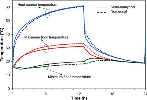
Figure 5 shows the time profiles of the heat source temperature (x = xq, y = 0), floor surface
maximum temperature (x = y = 0) and floor surface minimum temperature (x = 0, y = w/2) predicted by the semi-analytical and numerical models. The predictions of the semi-analytical model compare very well with those of the numerical model. The maximum difference is less than 11%. This difference may be attributed mainly to the non-uniform physical characteristics of the system, and partially to the employed mesh size in the numerical model, and the number of the retained series elements in the semi-analytical model. In fact, the case of a hypothetical system (not shown here) having uniform physical characteristics (e.g., slab without floor coverings and insulation) showed that the semi–analytical model is in excellent agreement with the numerical model.
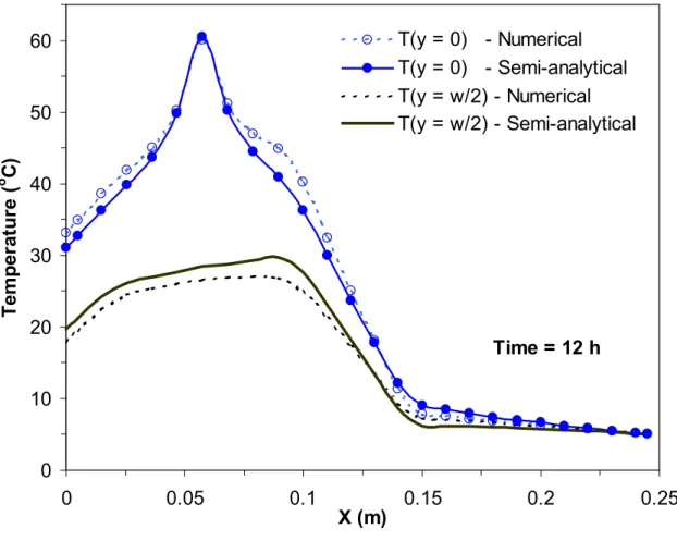
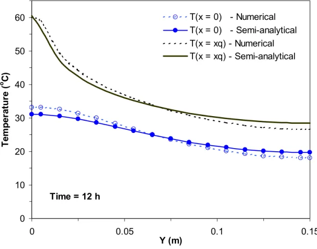
Figure 6 shows the temperature profiles of the left-side surface (y = 0), and the right-side surface (y = w/2) predicted by the semi-analytical and numerical models at the end of the heating cycle (time = 12h). Figure 7 shows the temperature profiles of the floor surface (x = 0), and a
horizontal surface passing through the heat source point (x = xq) predicted by the semi-analytical
and numerical models at the end of the heating cycle (time = 12h). Again, the predictions of the semi-analytical model compare very well with those of the numerical model. The maximum difference is less than 9%. As in the previous results, this difference is attributed mainly to the non-uniform physical characteristics of the system.
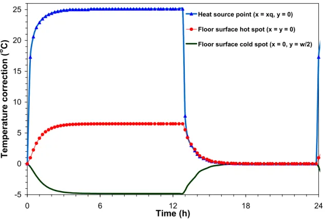
The previous graphs clearly showed that a multi-dimensional model should be used to accurately predict the thermal performance of radiant systems. To demonstrate the usefulness of a two-dimensional over a one–two-dimensional model, the semi-analytical model is used to calculate the temperature corrections (Φ values) for the heat source point, and floor surface cold and hot spots. Figure 8 shows these temperature corrections. The temperature correction for the heat source can reach up to 25°C, and that for the floor surface may fluctuate between -5°C to +6°C. This means that when a one-dimensional model is used, the thermal capacity of the system will be significantly oversized. Furthermore, thermal comfort may be jeopardized at the cold and hot spots (for heating systems), and moisture condensation at the cold spot may occur (for cooling systems).
The previous results were for an ideal case where the heat injection rate is fixed. In practice, however, the heat injection rate varies with time. To illustrate this effect, figure 9 shows the time-response of a hydronic system in terms of the water average and outlet temperatures (Tfm and
Tout) and the outside tube temperature (Tto) when coupled with the floor slab. The hydronic
system has the following characteristics: Di = 12mm, Dout = 16mm, kt = 0.1 W/m o
C, ρt = 1100
kg/m3, ct = 2000 J/kg oC. The system serves a surface area of 16m2 (with one circuit of a total
tubing length Lc = 53.3m). During a 12-hour heating period, the water enters the circuit tubing
with an inlet temperature Tin = 50°C with a volumetric flow rate of 1 liter/min. The system is
completely shut off during the rest of the day (m = 0). The system reaches the quasi-steady regime in about 2 hours. The water outlet temperature is about 8 degrees lower than the inlet temperature. The heat delivered from the boiler to the water (Qb) is completely transferred to the
concrete slab, except at the start of the heating period, suggestion minor thermal storage in the water and tubing masses. The heat transferred to the concrete slab (Qc) decreases about 32%
from the start to the end of the heating period.
CONCLUSION
A detailed model was developed for radiant heating and cooling systems for integration in energy simulation software. The model targets energy simulation software that use the one-dimensional numerical modeling to calculate the heat transfer within the building construction assemblies. The developed model is decomposed into two sets: one set uses the heat source method to calculate the heat transfer within the radiant medium, and the second set calculates the heat transfer within the circuit tubing. The heat transfer within the radiant medium is solved using the one-dimensional numerical modeling already built in the energy simulation software, and a two-dimensional analytical solution is appended to it. The heat transfer from the circuit tubing to the adjacent medium is solved using an analytical model. The two sets are coupled together via the temperature of the heat source node, i.e., the heat source node temperature equals to that of the circuit tubing outside surface. The advantage of this model over the one-dimensional model is that it accurately predict the circuit tubing-concrete contact surface temperature, which is required to compute the boiler/chiller thermal capacity, and the minimum and maximum ceiling/floor temperatures, which are required for moisture condensation (ceiling cooling systems), thermal comfort (heating floor systems) and controls. The model predictions compared very well with the results from a full, two-dimensional numerical model.
ACKNOWLEDGEMENT
This work was funded by the Institute for Research in Construction of the National Research Council of Canada, and Natural Resources Canada (CANMET/Buildings Group). The author is very thankful for their contribution.
REFERENCES
Kilkis B.I., Sager S.S., and Uludag M., A simplified model for radiant heating and cooling panels, Simulation Practice and Theory 2, pp. 61-76, 1994.Athienitis AK, and Chen TY,
Experimental and theoretical investigation of floor heating with thermal storage, ASHRAE Trans. 99(1), pp. 1049-1057, 1993.
Lisa L. M., Radiant heating provides energy-efficient versatility, Professional builder and remodeler, 1992.
Stetiu C., Energy and peak power potential of radiant cooling systems in US commercial buildings, Energy and Buildings 30, pp. 127-138, 1999.
Feustel H.E. and Stetiu C., Hydronic radiant cooling – preliminary assessment, Energy and Building, 22, pp. 193-205, 1995.
Yost P.A., Barbour C.E., and Watson R., An evaluation of thermal comfort and energy consumption for a surface mounted ceiling radiant panel heating system, ASHRAE trans. 101(1), pp. 1221-1235, 1995.
Simmonds P., Practical applications of radiant heating and cooling to maintain comfort conditions, ASHRAE Trans. 102(1), pp.659-665, 1996.
Simmonds P., Control strategies for combined heating and cooling radiant systems, ASHRAE Trans. 100(1), pp.1031-1039, 1994.
Olesen B.W., Comparative experimental study of performance of radiant floor heating systems and a wall panel heating system under dynamic conditions, ASHRAE Trans. 100(1), pp. 1011-1023, 1994.
Gibbs D.R., Control of multi-zone hydronic radiant floor heating systems, ASHRAE Trans. 99 (1), pp. 1003-1010, 1993.
Leigh S.B. and MacCluer C.R., A Comparative study of proportional flux-modulation and various types of temperature-modulation approaches for radiant floor heating system control, ASHRAE Trans. 100(1), pp. 1040-1052, 1994.
MacCluer C.R., The response radiant heating systems controlled by outdoor reset with feedback, ASHRAE Trans. 97(2), pp. 795-799, 1991.
Kollmar A. and Liese W., Die strahlungsheizung (R. Oldenbourg, Munchen, 4th ed., 1957).
Leal R.L.V. and Miller P.L., An Analysis of the transient temperature distribution in pavement heating installations, ASHRAE Trans. 78(2), pp. 71-78, 1972.
Zhang Z. and Pate M.B., A numerical study of heat transfer in a hydronic radiant ceiling panel, in numerical methods in heat transfer (eds., Chen J.L.S and Vafai K.), ASME-HTD, 62, 1986.
Zhang Z. and Pate M.B., A semi-analytical formulation of heat transfer from structures with embedded tubes, Heat transfer in buildings and structures (eds., Kuehn T.H.), ASME-HTD, 78, 17-25, 1987.
Athienitis AK, and Chen TY, Experimental and theoretical investigation of floor heating with thermal storage, ASHRAE Trans. Vol. 99, pt. 1, 1993.
Kilkis B.I., Eltez M. and Sager S., A simplified model for the design of radiant in-slab heating panels, ASHRAE Trans., pp. 210-216, 1995.
Kilkis B.I., and Sapci M., Computer-aided design of radiant sub-floor heating systems, ASHRAE Trans., pp. 1214-1220, 1995.
Kilkis B.I., and Coley M., Development of a complete software for hydronic floor heating of buildings, ASHRAE Trans., pp. 1201-1213, 1995.
Maloney D.M., Pederson C.O., and Witte M.J., Development of a radiant heating system model for BLAST, ASHRAE Trans. 94(1), pp. 1795-1808, 1988.
Strand R.K. and Pederson C.O., Implementation of a radiant heating and cooling model into an integrated building energy analysis program, ASHRAE Trans. 103(1), pp. 949-958, 1997.
Strand R.K. and Pederson C.O., Modeling radiant systems in an integrated heat balance based energy simulation program, ASHRAE Trans. 108(2), pp. 1-9, 2002.
Stetiu C., Feustel H.K. and Winkelmann F.C., Development of a Simulation Tool to Evaluate the performance of Radiant Cooling Ceilings, LBNL-37300, 1995.
Chun W.C., Jeon M.S., Lee Y.S., Jeon H.S. and Lee T.K., A thermal Analysis of a radiant floor heating system using SERI-RES, Int. J. Energy Res., 23, 335-343, 1999.
Miriel J., Fermanel F., and Mare T., Modeling of water ceiling radiant panel heating and cooling system – interaction between air velocity and temperature fields, Computational
technologies for fluid/thermal/structural/chemical systems with industrial applications, Vol. 1, pp. 285-291, 1999.
Incropera F.P. and De Witt D.P., Fundamentals of heat and mass transfer. 3rd Edition, John Wiley & Sons, Inc., 1991.
Patankar S.V., Numerical Heat Transfer and Fluid Flow, Hemisphere Publishing Corp., New York, 1980.
Concrete
Floor coverings
Rigid insulation
Conduction to ground
Convection to adjacent air Radiation to surroundings Gravel Concrete Floor coverings Rigid insulation Conduction to ground
Convection to adjacent air Radiation to surroundings
Gravel
Figure 1 Schematic description of a slab-on-grade floor radiant system
T
inT
outL
cslab surface
tubing
z
y
x
T
inT
outL
cslab surface
tubing
z
y
x
x
y
s
W/2
Averaging control volume xq
x
y
s
W/2
Averaging control volume xq
Figure 3 Calculation domain
dz
T
to
T
f
dQ
c
dQ
f
dQ
b
T
ti
dz
T
to
T
f
dQ
c
dQ
f
dQ
b
T
ti
0 10 20 30 40 50 60 0 6 12 18 24
Time (h)
Temperature (
oC)
Minimum floor temperature Heat source temperature
Maximum floor temperature
Semi-analytical Numerical
Figure 5 Profiles of the minimum floor temperature (x = 0, y = w/2), maximum floor temperature (x = y = 0), and heat source temperature (x = xq, y = 0) as a function of time -
0
10
20
30
40
50
60
0
0.05
0.1
0.15
0.2
0.25
X (m)
Tem
p
er
at
ur
e (
oC)
T(y = 0) - Numerical
T(y = 0) - Semi-analytical
T(y = w/2) - Numerical
T(y = w/2) - Semi-analytical
Time = 12 h
Figure 6 Temperature profiles of the left side surface (y = 0) and right-side surface (y = w/2) predicted at the end of the heating cycle (time = 12h) - comparison between the numerical and semi-analytical models
0
10
20
30
40
50
60
0
0.05
0.1
0.15
Y (m)
Tem
p
er
at
ur
e (
oC)
T(x = 0) - Numerical
T(x = 0) - Semi-analytical
T(x = xq) - Numerical
T(x = xq) - Semi-analytical
Time = 12 h
Figure 7 Temperature profiles of the floor surface (x = 0) and heat source horizontal surface (x = xq) predicted at the end of the heating cycle (time = 12h) - comparison between the
-5 0 5 10 15 20 25 0 6 12 18 24
Time (h)
Temperature correction (
oC)
Heat source point (x = xq, y = 0) Floor surface hot spot (x = y = 0) Floor surface cold spot (x = 0, y = w/2)
Figure 8 Temperature corrections (Φ values) calculated at the floor surface hot (x = y = 0) and cold (x = 0, y = w/2) spots and at the heat source point (x = xq, y = 0)
0
10
20
30
40
50
0
6
12
18
24
Time (h)
Temperature (
oC)
0
500
1000
1500
2000
Heating power (W)
Tfm
Tout
Tto
Qc
Qb
Table 1 Physical characteristics of a slab-on-grade radiant system Layer Thickness (m) Conductivity (W/m⋅K) Density (kg/m3) Specific heat (J/kg⋅K) Gravel bed 0.100 0.520 2050 184 Insulation (Polyestyrene) 0.050 0.027 55 1210 Concrete 0.10 0.38 1200 653 Floor covering (hardwood) 0.019 0.14 600 1210