Capturing the impacts of land use on travel behavior : comparison of modeling approaches

(1)

Capturing the Impacts of Land Use on Travel Behavior:

Comparison of Modeling Approaches

by

Veronica Adelle Hannan

B.S., Louisiana State University (2008)

Submitted to the Department of Civil and Environmental Engineering

and _ARCHNO

Department of Urban Studies and Planning ASECTS N E in partial fulfillment of the requirements for the degrees of F TECHNOLOGY

Master of Science in Transportation

I

_{NOV 12 2013}

12

and

Master in City Planning

IBRARIES

at the

MASSACHUSETTS INSTITUTE OF TECHNOLOGY September 2013

A u th or ... ...

Department of Civil and Environmental Engineering and Department of Urbyjtu ud aing

us 1 ,2 Certified by...

P. Christop er Zegras Associate Professor of Urban Planning, Transportation and,4ngineer* stems up rvisor

Accepted by ... ...

P. Christo e Zegras Associate Professor of Urban Planning, Transportation and Engineeri g ystems, Chair, Masteijin City Planr/ g6mmitgee A ccepted by ...

Heidi 1. Nbpf Chair, Departmental Committee for Graduate Students

(2)

(3)

Capturing the Impacts of Land Use on Travel Behavior: A

Comparison of Modeling Approaches

by

Veronica Adelle Hannan

Submitted to the Department of Civil and Environmental Engineering and

Department of Urban Studies and Planning on August 16, 2013, in partial fulfillment of the

requirements for the degrees of Master of Science in Transportation

and

Master in City Planning

Abstract

Most urban planning literature suggests that compact and mixed-use neighborhoods correlate with lower vehicle kilometers traveled (VKT), and accordingly, lower energy consumption and transportation-related emissions. However, many of these studies also find that the relationship between urban form and travel behavior is marginal at best, and several commit analytical errors, which may compromise the robustness of parameter estimates.

This thesis examines daily travel behavior in Santiago de Chile to understand how de-mographic structure, neighborhood design, and regional accessibility influence travel behavior as measured through emitted grams of five criteria pollutants (C0 2, VOCs, PM10, CO and NO,). To answer this question, two different modeling techniques

are employed to investigate the variables related to car ownership and travel behav-ior. The first analysis uses a discrete-continuous choice model to understand the attributes that influence car-ownership and travel emissions. The second study uses structural equation modeling to simultaneously estimate latent urban form factors, car-ownership and emitted pollutants. The advantage of each technique is that they both offer the flexibility to address the four major methodological errors identified in the literature review: inulticollinearity, spatial auto-correlation, the modifiable areal unit problem and self-selection.

(4)

After controlling for the four methods-related gaps, both models find that, although economic and demographic characteristics dominate in explaining travel decisions, the built environment plays a small, but significant, role. The discrete-continuous choice model uses two classes of measures to capture urban form: local attributes and regional accessibility. It finds that neighborhood-level and regional characteris-tics have an equally important impact on 2 or 3-plus vehicle ownership.Furthermore, the model suggests that regional accessibility attributes dominate among the built environment measures in explaining variations in emitted travel pollutants.

The structural equation model uses three latent urban form factors to characterize the built environment: a high-intensity, mixed-use factor; a high-income residential factor; and a non-gridded street factor. It finds that the high-density, mixed-use factor decreases the utility of owning a vehicle, and reduces the likelihood of travel emissions. The latter two factors, on the other hand, both increase the probability of owning a car. Lastly, the non-gridded street factor has a consistently positive effect on travel emissions.

Thesis Supervisor: P. Christopher Zegras

Title: Associate Professor of Urban Planning, Transportation and Engineering Sys-tems

(5)

2.2.1 Land Use Data . . . . 2.2.2 Demographics and Travel Behavior . . 2.2.3 Household Travel Emissions . . . . 2.3 Measures and Descriptive Statistics . . . . 2.3.1 Spatial Unit . . . . 2.3.2 Built Environment Measures . . . . 2.3.3 Endogenous Variables . . . . 2.4 Final Data Checking . . . . 2.4.1 Variance Inflation Factor . . . . 2.4.2 Kaiser Measure of Sampling Adequacy

. . . . 47 . . . . 53 . . . . 54 . . . . 55 . . . . 55 . . . . 56 . . . . 60 . . . . 61 . . . . 61 . . . . 62 . . . . 67 . . . . 68 . . . . 68 . . . . 68

3 HOUSEHOLD VEHICLE OWNERSHIP AND TRAVEL EMISSIONS 73 3.1 Discrete-Choice Model Estimation 3.2 Results . . . . 3.2.1 BNL Model ... 3.2.2 MNL Model ... 3.2.3 Multi-Variate Regression 3.3 Demand Elasticity ... 3.3.1 Elasticity Measures . . . 3.3.2 Selected Elasticities . . . 3.4 Spatial Autocorrelation . . . . . 3.5 Summary . . . . 4 CHARACTERIZING URBAN FORM THROUGH LATENT FAC-TORS: . . . . 7 4 . . . . 74 . . . . 7 5 . . . . 78 . . . . 8 3 . . . . 8 8 . . . . 8 8 . . . . 8 9 . . . . 9 1 . . . . 9 9

(7)

A STRUCTURAL EQUATION MODELING 4.1 Statistical Analysis ...

4.2 R esults . . . . 4.2.1 Exploratory Factor Analysis ...

4.2.2 Confirmatory Factor Analysis ... 4.2.3 SEM ...

4.3 Sum m ary ... ....

APPROACH

5 Conclusions and Policy Implications

5.1 Introduction . . . .

5.2 The link between land use, vehicle choice, and travel emissions

5.2.1 Neighborhood-level Effects . . . .

5.2.2 Relative Location Effects . . . .

5.2.3 Additional Considerations . . . .

5.3 Policy Im plications . . . .

5.3.1 Policies aimed at potential first-car households . . . . .

5.3.2 Policies targeting the growth of multi-car households

5.3.3 Policies aimed at reducing emissions . . . .

5.4 Successes, shortcomings and future research . . . .

101 102 104 104 106 108 115 123 123 124 124 125 126 126 126 127 128 129

(8)

(9)

List of Figures

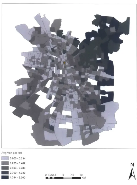
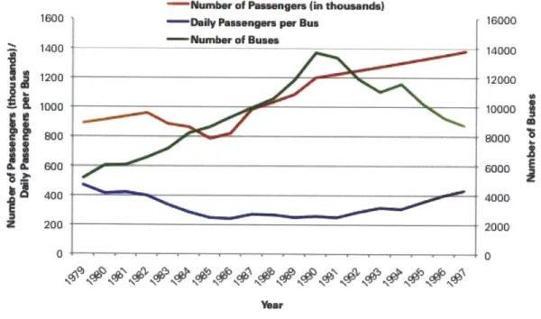
2-1 Income Distributions at Two Slices in Time: 1991 and 2001 . . . . 2-2 Household Vehicle Ownership . . . . 2-3 Auto m ode share . . . . 2-4 Bus Ridership and Fleet Growth in the 1980s and 1990s . . . . 2-5 Bus and Metro Fares in Santiago de Chile

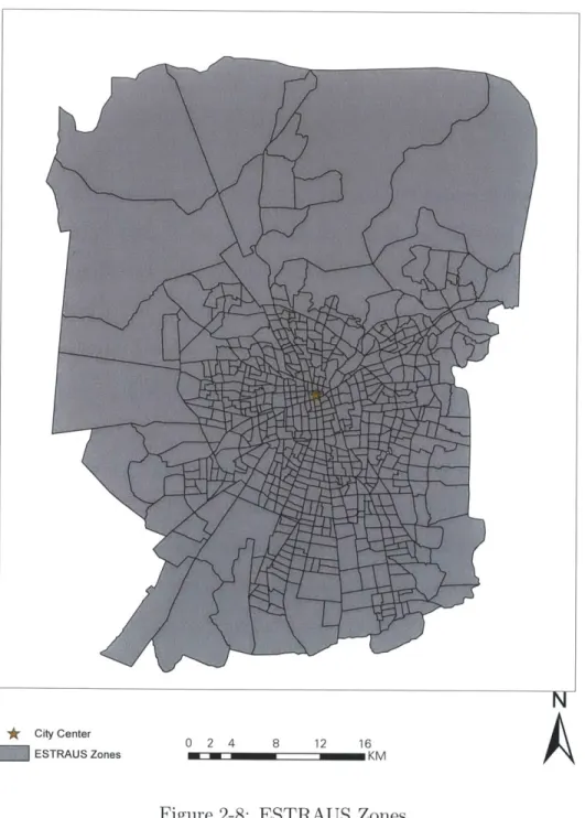
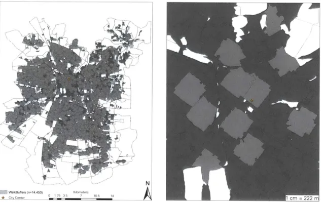
Metro Ridership and Infrastructure 2001 Travel Survey Sampled Zones ESTRAUS Zones . . . . Walk Buffers . . . .

CO2 Path Diagram . . . . VOC Path Diagram . . . . PM0 Path Diagram . . . .

CO Path Diagram . . . . NO., Path Diagram . . . .

Growth over Time: 1970s to 2000 54 . . . . 5 6 . . . . 5 9 . . . . 6 2 . . . 1 18 . . . 1 19 . . . 120 . . . 12 1 . . . 12 2 47 49 50 51 . . . . 53 2-6 2-7 2-8 2-9 4-1 4-2 4-3 4-4 4-5

(10)

(11)

List of Tables

2.1 _{Variables, Definitions, Units, Descriptive Statistics and Expected} Cor-relation with Vehicle Ownership or Travel Emissions . . . . 2.2 Variables, Definitions, Units, Descriptive Statistics and Expected

Cor-relation with Vehicle Ownership or Travel Emissions (cont'd) . . . . . 2.3 _{Kaiser Measure of Sampling Adequacy Scores . . . .} 3.1

3.2 3.3

BNL Model Results ...

Multinomial Logit Model Results . . . . OLS Model of Household Survey Day Travel Emissions (grams) 3.4 Elasticities of Household Travel Pollution

Diagnostics for Spatial Dependence . . . . CO2 Spatial Error Model . . . . CO Spatial Error Model . . . . NO, Spatial Error Model . . . . PM10 Spatial Lag Model . . . .

Comparison of Fit Measures . . . . EFA of Built Environment Characteristics (n=7,225) CFA of Land Use Characteristics (n=7,222) . . . . . Final CFA of Land Use Characteristics (n=14,447) Binary Vehicle Choice Model Results (n=14,447)

. . . . 9 1 . . . . 93 . . . . 94 . . . . 95 . . . . 96 . . . . 97 . . . 107 . . . . 108 . . . . 110 .. .... 111 70 71 72 76 82 87 90 3.5 3.6 3.7 3.8 3.9 3.10 4.1 4.2 4.3 4.4

(12)

(13)

List of Abbreviations

3D's Density, Diversity and Design BNL Binomial Logit

CBD Central Buisness Distict CFA Confirmatory Factor Analysis CFI Comparative Fit Index

CO Carbon Monoxide

CO2 Carbon Dioxide

EFA Exploratory Factor Analysis El Entropy Index

FAR Floor to Area Ratio GDP Gross Domestic Product GHG Green House Gases IV Instrumental Variable

LISA Local Indicator of Spatial Association MAUP Modifiable Areal Unit Problem ML Maximum Likelihood

MLR [Robust] Maximum Likelihood estimator MNL Multinomial Logit

NOx Oxides of Nitrogen OLS Ordinary Least Squares PM10 Particulate Matter

(14)

RMSEA Root Mean Square Error SC Schwarz Criterion

SEM Simultaneous Equation Modeling

SRMR Standardized Root Mean Square Residual TAZ Traffic Analysis Zone

TLI Tucker Lewis Index

UTM Universal Transverse Mercator VIF Variance Inflation Factor VKT Vehicle Kilometers Traveled VMT Vehicle Miles Traveled

(15)

1 1

REVIEW OF LITERATURE

1.1 Introduction

This thesis is an exploration of interaction between transportation and land use in Santiago de Chile. Skyrocketing motorization rates are one of the biggest threats to the sustainability and prosperity of the industrializing world. Although these motor-ization rates are partially driven by GDP growth per capita, there are more nuanced, and potentially avoidable, causes of this increased demand for private vehicles. A growing body of literature suggests that there is an undeniable association between the built environment and travel behavior. This thesis aims to examine those rela-tionships in more detail, and tests the hypothesis that deliberate urban planning is a promising mechanism for reducing motorization rates.

It builds on existing research in two important ways. First this study examines the importance of neighborhood specification, and uses an empirically derived walk buffer to define a small and unique neighborhood for each sampled household. Sec-ond, this analysis corrects for the four principal errors committed in relevant analyses: multicollinearity, spatial auto-correlation, the modifiable areal unit problem and

(16)

self-selection. It uses two different modeling techniques to identify and quantify the ef-fects of different attributes on car ownership and travel behavior as evidenced through travel emissions. The first employs a widely used discrete-continuous framework to establish baseline estimates. The second technique examines the potential of simul-taneously estimating vehicle choice, travel emissions and latent land use factors in a structural equation model. After evaluating the utility of each analytical framework, the thesis ends with a discussion of the most salient findings, and their implications for future policies and development strategies.

1.2 The Rise of the Automobile

Rising incomes and an increased demand for mobility have caused a rapid increase in automobile ownership. This is especially true in developing countries, where motor-ization rates are far from saturation, and are forecasted to increase more than 10% per year

([341).

Likewise, VKT is also growing at unprecedented rates. According to Schafer, in 1960 individuals traveled an average annual distance of 1860 km. By

1990, that number had nearly tripled, and is predicted to increase at a global average rate of 8% per year ([61]).

The costs of rising automobile ownership are high. At the most basic level, increased motorization rates and higher auto mode share lead to congestion. As Gakenheimer explains, transportation supply cannot keep up with this combination of increased urbanization and motorization rates, and population and GDP growth,. Thus this has resulted in a traffic epidemic in nearly all developing countries ([34]).

(17)

Unfortunately, the effects of auto growth are not limited to roads. Despite innovations in transport technology and fuel formulations, energy consumption and greenhouse gas emissions (GHG) from the transportation sector are rapidly increasing across the globe. Presently, the transportation sector accounts for approximately 20% of all energy use, and it is almost exclusively dependent on petroleum-based fuels. It produces about 25% of all GHG, and is a leading contributor of other types of air pollution. In the United States, for example, transportation produces 40% of volatile organic compounds (VOC), 77% of carbon monoxide (CO), 49% of nitrogen oxides, and is a significant source of PM10. Within urban environments these percentages

tend to be higher, and characteristics, such as an aging vehicle fleet, poor vehicle maintenance or inappropriate fuel choices, drastically swings these averages

([37]).

Furthermore, there are numerous indirect effects of higher auto mode share. Many researchers contend that the rise of the automobile enabled sprawl and intrinsically changed the spatial character of cities, for the worse. Many researchers in the field of public health also argue that high auto mode share and long commute times are one of the many contributors to the global obesity epidemic

([32],

[68]).

Despite the well documented problems associated with vehicle ownership and use, the global desire for cars seems largely unchanged. Irrespective of cultures, geogra-phy or decade, there is a strong positive correlation between income, VKT, and traffic volume per capita

([61], [34]).

Thus, this trend has prompted researchers to explore vehicle ownership and travel behavior in more depth to understand what other factors might mitigate auto use without stifling economic growth.

(18)

1.3 The Land Use and Transportation Link

An extensive body of urban planning literature examines the interactions between land use and travel behavior. Typically, urban planning researchers tend to simplify

their characterization of the built environment by categorizing the elements of the built environment into a few key dimensions. Cervero and Kockelman classified these physical effects as the 3D's: density, diversity and design (1211). In 2009, Cervero et al. expanded the list to include two additional D's: distance to transit and destina-tion accessibility

(122]).

The following paragraphs contains a small selection of the notable findings regarding land use and transportation. For a more comprehensive review, see Ewing and Cervero ([29]

[30])

Density is always measured per unit area, though its exact specification can take many forms: employment density, dwelling unit density, population density, etc. Past research shows evidence of a link between high densities, lower car ownership and use, and higher transit share. In 1997, Cervero and Kockelman found that residen-tial density was negatively correlated with non-work VMT in the San Francisco Bay Area([21]). Similarly, in 2004, Zhang found that employment density at the work location increased an individual's likelihood of commuting by public transportation. Furthermore, there are numerous studies that find density strongly correlates with lower auto ownership rates. Cambridge Systematics published two studies (one based in Philadelphia, the other in San Francisco) that found that both dwelling unit den-sity and population denden-sity reduced the likelihood of owning a vehicle ([64], [65]). Likewise, Kitamura et al.

([441)

found a similar correlation between residential den-sity and vehicle ownership in Southern California. In 2010, Zegras found that higher

(19)

dwelling unit densities have marginal to notable effects on the decision to own 1, 2 or 3 vehicles in Santiago de Chile([69]).

Diversity refers to land use diversity, and is usually measured through a derived index aimed at capturing the proportion of different land uses present in a given area. Higher land use diversity shows evidence of being related to shorter trips, and fewer trips by private vehicles. In 2002, Hess and Ong

([391)

found that land use diversity decreased the likelihood of automobile ownership in Portland, OR. Using data from the metropolitan area of Hamilton, Canada (a suburb of Toronto), Potoglou and Ka-naroglou developed a disaggregate modification to the entropy index (EI) , computed as:

El₅_{oo =}

7k)

where, Pk _{is the proportion of the developed land in the kth land-use type, and 500}

denotes the 500m buffer distance used. They found the land use entropy measure had a negative impact on owning two or more vehicles

([59]).

There has also been com-pelling evidence that high land use diversity has a powerful impact on mode choice. In 1997, Cervero and Kockelman found that use mix, and high land use intensity both reduced the probability of choosing a single-occupancy vehicle in the San Francisco Bay Area.

Design captures the nature of the street network and the experiential elements of place. A street network may range from a dense, urban grid of four-way intersections to a sparse suburban network dotted with three-way intersections and dead ends. Design can also include sidewalk coverage, average building setbacks, street widths,

(20)

street trees or other physical attributes of a place. Cervero with others has published numerous studies demonstrating that design has a powerful and positive impact on non-motorized travel. In 2003, he and Duncan found that a "bike-friendly factor," which loaded heavily on small block sizes and high four-way intersection densities, moderately increased the likelihood of choosing a bike trip in the Bay Area ([201). In 2009, he analyzed non-motorized travel in Bogotd for an international perspective, and found that street density, connectivity and cycle tracks were the strongest predic-tors of non-motorized travel

(122]).

Zhang examined the effects of street connectivity in Boston, and found a negative association between proportion of cul-de-sacs, and public transportation or non-motorized trips. Similarly, he found that reduced net-work connectivity at the trip destination increased the likelihood of driving

(1731).

Furthermore, a large body of research points to a significant relationship between vehicle use and street design. In 2010 Zegras found that four-way intersections per linear km had a negative impact on owning two or more vehicles and VKT in Santi-ago. He also found that three-way intersections had a positive effect on VKT([69]).

Distance to transit and destination accessibility both capture a location's greater regional accessibility, and together these measures proxy for the ease of access to destinations. Numerous studies suggest that public transit provision is negatively correlated with VKT and car ownership ([69], [731, [22]) Furthermore, several stud-ies suggest that regional accessibility measures, such distance to CBD, are positively correlated with vehicle ownership, trip distances and trip frequencies

([691,

[15], [54],

1551).

Thus, although the connection between the built environment and travel be-havior is complex and still under examination, there is already considerable evidence that a correlation between these two entities exists.

(21)

1.4 The Built Environment and Energy Use

Studies analyzing the effects the urban form and energy use date back to as early as the 1970s. Anderson et al. provided a comprehensive review of this research, and con-cluded that the link between the built environment and energy use is equally tenuous as the relationship between urban form and travel behavior

([5]).

Many of the studies use CO2 as the outcome in question, and each study relies on very different datasets,

methods and assumptions, thereby creating the need to interpret these findings with caution. For example, Newman and Kenworthy published one of the earliest studies on density and energy use. Using data from an international selection of cities, they found a strong negative relationship between population density and transportation energy consumption per capita. Unfortunately, this analysis drew from inconsistent data sets and did not include socio-economic controls, which compromised the relia-bility of parameter estimates

([56]).

A new wave of energy use and urban form literature has tried to to incorporate more sophisticated controls into their analyses. In 2008, Glaeser and Kahn used descriptive analysis with controls for income, weather and density to examine the effects of urban form on CO2 in 66 metropolitan areas in the United States. They

found that transportation CO2 emissions per household were significantly higher in

low-density, sprawled regions, when compared with older, dense metropolitan areas

(135]).

Similarly, Brownstone and Golob used a broad range of socio-economic vari-ables in their analysis. They concluded that once they controlled for socio-economic variations, density still had a modest effect on annual vehicle miles traveled (VMT) and CO2 emissions. (118]).

(22)

1.5 Analytical Approach

Although the existing literature suggests that compact development coupled with a balanced mix of land uses correlates with lower VMT, motorization rates and trans-portation emissions, the relationship is weak and requires further analysis. Discrete-continuous choice models are a popular framework for understanding vehicle holding and use decisions. Although these models can be coupled with certain statistical cor-rections to produce precise and robust parameter estimates, they are not capable of robustly capturing highly complex and interconnected relationships between indepen-dent and depenindepen-dent variables. Simultaneous Equation Modeling (SEM) , on the other hand, is a less-explored modeling technique that allows researchers to relax some of these commonly violated assumptions, and accurately model complex indirect and direct relationships.

Sections 1.5.1 and 1.6.1 will provide a theoretical background on both of these analysis techniques. They will discuss the estimation methods and review how these techniques are applied in current urban planning literature. Then Section 1.7 will conclude with an overview of the principal analytical shortcomings committed in urban planning publications, and how those issues can be addressed using discrete-continuous choice models or SEM.

1.5.1 Discrete Choice Models

Discrete choice models characterize and predict choices between two or more distinct alternatives. They use empirically-derived data sets to reflect disaggregate

(23)

prefer-ences and allow for a more nuanced examination of decision-making.

According to Ben-Akiva and Lerman ([13]), individuals will select the alternative that maximizes their utility. Because utility is an abstract concept, it is modeled as a random variable, U, in which n individuals will select from

j

alternatives:

Uin = V(Zjn, Sn, /) + 6in (1.2)

where V is the systematic utility expressed as a function of a vector of attributes, Zin, and a vector of socioeconomic characteristics sn that are unique to each alternative

j

for n individuals.

#

_{is a set of unknown parameters that are estimated statistically} to represent the effect of each variable on the probability of choosing an alternative (in this case, the choice is between 0, 1, 2, or 3 or more vehicles). 6_jn_{is the random}

utility component, which captures an analysts' imperfect knowledge resulting from unobserved attributes or preferences, or imperfect measurements. Utility is modeled as a probability of choosing alternative i from choice set, Cn

P (i|IC) = P (maxj Un, Vj E Cn) (1.3)

As Equation 1.3 suggests, the choice probability depends on the differences between alternatives and is not an absolute value.

The logit model is one of the most widely used discrete choice models because the formula for the choice probabilities takes a closed form and is readily interpretable.

(24)

The logit probabilities can be expressed as

P . = (1.4)

Representative utility is usually specified to be linear in parameters: Vnj = 'Xnj, where xj is a vector of observed variables relating to alternative

j

([13],

[111).

Ac-cording to McFadden

(511)

the log-likelihood function with these choice probabilities is globally concave in parameters 3. This facilitates numerical maximization meth-ods and allows numerous computer packages to estimate logit models

([51]).

In this thesis, Biogeme was used to estimate the binary and multinomial logit models

([141).

1.6 Discrete-Continuous Modeling Framework

In urban environments, vehicle use is an equally important consideration as vehi-cle ownership. Unfortunately, properly estimating these decisions requires a more complex analytical framework. Many studies suggest that the correlation between demand for certain goods, such as electricity, vehicle kilometers traveled (VKT) or travel emissions, may be biased by a key, but not directly observed, factor. For ex-ample, the decision to own a bicycle and to bike numerous kilometers everyday may both be driven by an unobserved preference for cycling. Therefore, in the cases where the factors determining the demand for an item are highly correlated with the factors predicting its use, more sophisticated modeling techniques must be used to avoid

in-consistent estimates (126],

[50]).

(25)

(here, individuals "choose" their travel emissions through their trip characteristics, e.g. mode choice, trip time, frequency, destination etc.):

Yij = oiX3 + vt (1.5)

where

yij = _{travel emissions per households, measured in kg;}

0, = vector of household characteristics;

Xi = a vector of estimable parameters that vary for each pollutant; and

vj = unobserved characteristics of the household;

The problem of endogeneity emerges because Ep in Equation 1.2 and vij from Equa-2 tion 1.5 are correlated due to an omitted variable, simultaneity or reverse causality bias. For example, a household's innate enjoyment of motor vehicle travel (and high level of emitted grams C02) will undoubtedly impact its probability of owning one or more automobiles. Likewise, the unobserved attitude of driving displeasure, would increase the utility of owning zero vehicles, and make a household more likely to limit motor vehicle travel and have lower emissions.

If the error terms in a discrete-continuous choice model are related, then estimating Equation 1.5 with ordinary least squares (OLS) will produce biased and inconsis-tent results. One option for avoiding inconsisinconsis-tent parameter estimates is to model emissions with a correction factor to counter the effects of the estimation bias. Sev-eral effective correction tactics have already been developed. Mannering and Hensher compiled a survey of these procedures, and found that they vary widely in their

(26)

com-putational intensity and practicality. They also noted that the correction techniques generally fell in two categories: indirect and direct methods. Indirect methods use econometric techniques that were developed to address simultaneity, and they are commonly implemented as an instrumental variable. Although Mannering observes that this technique has the benefit of simplicity, he cautions that alternative correc-tion techniques can result in more precise parameter estimates.

Direct methods are the other class of analytical techniques that can be used to address endogeneity. They require some interaction between the discrete and continuous por-tion of the modeling framework. Of the methods Mannering and Henscher examined, they found that using the expected value of operating cost to correct for unobserved bias was not only one of the most flexible methods being reviewed, but also one of the easiest to apply. Moreover, it has been successful in numerous published articles (see [26], [411, [50]) and obtained near identical results to more complex techniques([49]).

Deriving the expected value starts by estimating the discrete choice model for the consumer good of interest. The probabilities from the output file are then inserted into the following equation to derive the expected value:

n

E (X) = (k - P (X - Xk)) (1.6)

k=1

where

x = operating cost of alternative k; and

(27)

Finally, emissions (yij) are estimated using E (X) in place of a dummy variable for the number of motor vehicles.

1.6.1 Structural Equation Modeling

Measurement constraints have traditionally limited urban planning researchers to quantifying the built environment through a combination of independently measured attributes. Recently, that characterization of land use has been become increasingly contested, and several researchers maintain that combinations of variables may have a greater influence on the decision-making process

(121],

[29], [1]).

There are already many examples of using latent land use constructs in OLS and discrete choice models ([21],

[29],[63]).

_{The outcomes of these studies suggest that the built environment} follows somewhat predictable land use patterns. For example, the CBD is typically characterized with high-density development that concentrates offices and services. Residential neighborhoods on the other hand, are characterized by residential and educational land uses, and typically have more green space and a higher percent-age of local streets. In the United States and some other parts of the global north, distinct land use patterns have also been connected with neighborhood age, where older neighborhoods (those built before the 1920s) tend to exhibit high-density and mixed land use. Newer neighborhoods (especially those built after 1960) tend to be single-use, and characterized by wider roads and low densities. Factor analysis analysis allows for a more statistically complex grouping of variables that does not have to classify neighborhoods on a single parameter (age, function etc.). Instead it uses covariance and variance matrices to understand if urban form follows any latent patterns, and it helps researchers understand if these latent patterns better represent potential relationships between the built environment and travel behavior.

(28)

Another motive for using SEM is that it avoids inconsistent estimates that may result from using the latent factors in another equation without their error terms

(12]).

SEM resolves this problem, because it simultaneously estimates a system of equations and gives researchers the freedom to specify variables as both endogenous

and exogenous. A structural equation system can be expressed as

y = a + By+ Fx+ (1.7)

where

y =vector of p endogenous variables x =vector of m exogenous variables a =vector of regression intercepts

B =p x p matrix parameter matrix of regression coefficients for the equations directly relating

the endogenous variables

F =p x m matrix parameter matrix of regression coefficients for the equations relating the endogenous and exogenous variables.

vector of p disturbances

SEM models are estimated by applying matrix algebra to the variance-covariance ma-trix. The objective-function is to minimize the differences between the model implied variance-covariance matrix and the original sample's variance-covariance structure. ([1]). Covariances-based estimation assumes that the covariance matrix of the

(29)

served variables is a function of a set of parameters as illustrated in Equation 1.8:

()(1.8)

where

= _{population covariance matrix of observed variables,}

0 = vector of model parameters, and

(0) = covariance matrix written as a function of 0

The matrix E

(0)

has three components:

1. the covariance matrix of Y

2. the covariance matrix of X with Y

3. the covariance matrix of X

Depicting 4 as the covariance matrix of X, and T as the covariance matrix of , then according to Bollen 1989, the model parameters can be estimated using the following matrix of equations:

(1.9) () (I - B)- 1 (FP4F' + T) (I - B)-" (I - B)

1AF

1

4 F' (I -

B)-Proper estimation is contingent on model identification, which requires that unique estimates of model parameters be obtained. This limitation is addressed by incorpo-rating a theoretical understanding of the phenomena to restrict model parameters.

(30)

For further discussion of model identification, see [171, 125], or [461

1.7 Methodological Challenges

The advantage of discrete-continuous choice models and SEM is that they can both be employed in disaggregate studies that include a wide variety of socioeconomic controls. However, the nature of urban data presents numerous technical challenges that are not immediately addressed in these estimation methods. For example, many of the dimensions used to characterize the built environment are highly correlated with one another. Moreover, there are no universally agreed upon methods for data aggregation, and the analysis always risks omitting a key variable, such as local or regional effects, or some unobserved latent preference. Furthermore, although many of the studies cited in Section 1.3 found a correlation between the built environment and travel behavior, they say nothing about causality, and do not account for the fact some unobservable characteristic might influence both travel behavior and residential location. In light of these analytical shortcomings and mixed empirical findings, fur-ther examination of land use and transportation interactions are required. This thesis will address the four most common methodological challenges: spatial autocorrela-tion; the modifiable areal unit problem (MAUP); multi-collinearity; and endogeneity and self-selection. They are discussed in brief in the next sections.

1.7.1 Spatial Auto-Correlation

Spatial autocorrelation is a phenomena where a variable, or the error term of a pre-dicted outcome is correlated with itself in space, thereby violating the assumption of independence in observations. If neighboring samples are more alike, there is positive

(31)

spatial autocorrelation. On the other hand, negative spatial autocorrelation arises when nearby areas are distinct from one another.

Several corrections have been proposed to address spatial effects. A widely used approach is the one developed by Anselin

([7]),

which can be written in matrix form as follows:

Y =pWY+X# + (1.10)

E = AWe+,p (1.11)

where,

Y = an n x _{1 vector of objective variable observations,}

X = an n x K matrix of independent variable observations,

0 = a 1 x K vector of parameters corresponding to K independent variables,

p = a parameter of spatial association corresponding to the objective variable, A = a parameter of spatial association corresponding to c,

E = error term,

y = independent and potentially homogenous error terms, and

W = an n x n matrix containing weight wi that describe the interrelationships of different locations, i and

j.

The advantage of this correction technique is that it is easily applied to the outcomes of a discrete-continuous model.

Treatment of spatial autocorrelation requires a two stage modeling process. The first step starts with a traditional regression model that is tested against a statistic of spatial association (see section 1.7.1). If this stage of modeling fails to find

(32)

signif-icant spatial association, then one can conclude the specified model accounts for all observed variability. Otherwise, a spatial model would have to be estimated ([57]) . For a detailed discussion regarding estimation and interpretation of these models, see Anselin ([7]).

Spatial Statistics

Two popular spatial statistics are Moran's I and Anselin's LISA (Local Indicators of Spatial Association, [81). Moran's I is a global statistic that measures spatial dependence. It can be expressed as

n Ei E, Wij (Yi - 9) (Yj - (1)2

I = En-_____ (1.12)

where

wij = weight matrix,

yi =value at the ith location, 9 mean value, and

n total number of observations

The Moran's I distribution is associated with a z-score, which tests the null hypoth-esis that values are randomly distributed across the study area.

The LISAstatistic is a local version of Moran's I that measures spatial dependence in portions of the study area. Rather than outputting a single score, the LISA statistic outputs a map grouping samples or regions into one of the following outcomes:

e High-high - when xi is above the mean and the values of xj in adjacent zones are also positive. This results in a positive statistic.

(33)

" Low-low - when both values are low. This results in a positive statistic. " High-low - when the value at i is above the mean and the values in surrounding

zones are below the mean. In this case, the statistic is negative.

" Low-high - when the value at i is below the mean and the values in surrounding zones are above the mean. This statistic is also negative.

" Not significant

Paez and Anselin recommend that researchers address spatial autocorrelation through a multi-stage approach

([57],

[7]).

The first stage begins by testing the results of the original OLS model with diagnostics for spatial dependence, and further supplement-ing this information with qualitative LISA cluster and significance maps. If Moran's

I is significant, the Lagrange Multiplier test is used to determine whether a spatial

error or spatial lag model should correct for spatial autocorrelation. Traditionally, spatial lag is best suited for addressing phenomena where neighboring values influence each other through migration or diffusion processes. Spatial error, on the other hand, controls for spatial mismatch and omitted variables

([9]).

Chapter 3 followed this procedure to account for spatial dependence, and addressed spatial autocorrelation through both spatial lag and spatial error models. All analyses were conducted in Geoda, an open source software program developed by Anselin that specializes in spatial data analysis and geovisualization

([8]).

1.7.2 MAUP

Land use and transportation research often uses aggregated data sets, which creates the potential for spatial misrepresentation. The MAUP arises because there is an infinite number of ways a region can be subdivided, and each classification strategy

(34)

can result in different reported outcomes. There are two main sources of error in the MAUP: scale error and the zoning effect. Scale error is a function of different levels of aggregation, which potentially mask the study region's variation through excessive averaging. The zoning effect, on the other hand, emerges when different boundary conditions lead to very different depictions of a place, as a result of a different aggre-gation schemes capturing cultural, demographic, geographic, etc. differences better than others (157]).

In urban planning research, neighborhoods are generally defined by institutional boundaries: either census tracts or block groups, zip codes, or Traffic Analysis Zone

(TAZ),

etc. depending on the data the researcher has available to him or her. Al-though these boundaries provide analytical convenience, they are mis-leading con-structs in micro-level causal analyses. These predefined zones often follow population-driven zoning schemes which mask demographic, economic or behavioral sample vari-ation. Furthermore, these artificial and arbitrary boundaries may not reflect a res-ident's perception of his or her neighborhood, which undoubtedly plays a role in influencing people's travel behavior. According to Clark (123]), the effects of data variation are best addressed by grouping observations in a manner that results in minimal information loss. Ideally, this would be accomplished by employing a tech-nique that combines the data into homogeneous sub categories. Paez further suggests that researchers should starts with the smallest zones possible, and compare the ini-tial results with increasingly aggregated zoning strategies to ensure the results are robust over a wide range of aggregation schemes ([57]).

(35)

1.7.3 Multicollinearity

Another challenge in urban planning research is the significant level of correlation among design, density, diversity and destination accessibility measures. For exam-ple, compact neighborhoods are also likely to have dense street networks and mixed land uses. As a result of these pervasive interrelationships, a regression that includes too many measures of the built environment, risks violating a core assumption of OLS regression: no variable can have an exact or near exact linear relationship with another independent variable

([58]).

Otherwise, incorporating two or more highly re-lated variable will result in biased and inconsistent least-squares parameter estimates.

One approach to addressing multicollinearity is to condense the offending variables into an index. Frank

([33])

developed a walkability index to capture the effects of the built environment on walking behavior. To develop his measure, he computed a z-score for net residential density, land use mix and intersection density, and combined those values into a single score via a weighted average. Although, he found that the walkability index positively correlated with physical activity, his approach was cum-bersome and required trial-and-error tests to determine the optimal parameters for the weighted average.

Factor Analysis is another approach to creating a multidimensional index of neighbor-hood attributes. It used similarities in variance and covariance matrices to transform sets of highly-correlated attributes into a small number of unrelated or marginally related factors. In 1997, Cervero and Kockelman used factor analysis to transform various measures of the built environment, into two intuitive, but not easily

(36)

quan-tified, factors: walking quality and intensity. They found that these two factors had a marginal influence on non-work trip mode choice ([21]). Similarly, Bagley and Mokhtarian (2002) used factor analysis to create continuous measures of the

'traditional-ness' and 'suburban-ness' of sampled neighborhoods. These two factors

resulted from a combination of 18 characteristics, such as parking availability, dis-tance to grocery stores, presence of a grid street network and walking quality. More recently, in 2008, Ewing et al. used principle component analysis to reduce six ob-served variables relating to population densities and block size into a single index measuring sprawl. They found that the proxy for sprawl had a small but significant correlation with minutes walked, obesity and hypertension.

Drawing from past examples, this thesis aims to avoid the shortcomings of prior research by addressing multicollinearity in two ways. First, in Chapter 3, individual measures of built environment were inserted into a discrete-continuous model predict-ing auto ownership and travel emissions. Second, past research implies that factor analysis is a viable means of accurately characterizing the built environment without violating key statistical assumptions. Chapter 4 uses factor analysis as a part of structural equation modeling framework to understand land use and travel behav-ior interactions. It replaced the individual indicators of the built environment with three marginally correlated, multidimensional measures of the built environment. For

additional information on this technique, see Section 4.2.1

1.7.4 Endogeneity and Self-Selection

Although much of city planning literature suggests that a measurable correlation between urban form and transportation exists, there is a comparatively limited

(37)

un-derstanding of causality. Before researchers can be confident in the precision of their estimates and in the strength of their models, these shortcomings, known as self-selection and endogeneity, need to be addressed.

Self-selection is a phenomena that arises when individuals actively choose a situation based on inherent preferences or attitudes. It is partially caused by cross-sectional data sets, which cannot capture causality in a single time slice. Thus, although nu-merous studies have found that low density, suburban environments correlate with more driving and less public transportation share, it is not clear whether the observed travel outcomes can be ascribed to the built environment or existing travel prefer-ences. Although self-selection is starting to receive increasing consideration in urban planning literature, no consensus exists on how to accurately capture, quantify or correct for self-selection. The next section reviews the type of errors that result from self-selection and discusses the possible approaches to addressing this issue.

Despite the obvious challenges with trying to quantify or model the decision-making process, disregarding self-selection could lead to substantial analytical inaccuracies. In the model,

y- =3o + f1xi + Ej (1.13) OLS estimation assumes that the values, xi are uncorrelated with the error terms ci. If that assumption holds, then the attribute is exogenous and independent of any other variable within the system. However, if correlation exists between xi and ej,

(38)

In urban planning research there are two predominant sources of endogeneity. The first is omitted variable bias. As the name implies, this phenomena arises when an-other variable correlates with x and y. For example, attitudes, rather than the built environment, may cause an individual to choose a certain neighborhood type and a mode based on an overlooked latent preference for walking and high density, or driving and open space. The second is simultaneity bias, which arises when the in-dependent variable is jointly decided with the in-dependent variable. In both of these cases, endogeneity produces biased estimates of 3 and prevents researchers from as-signing causality.

Cao and Mokhtarian preformed one of the most comprehensive examinations of the empirical findings in studies that address self-selection([19]). They reviewed 38 empir-ical studies using nine different methods to control for self-selection: direct question-ing, statistical control, instrumental variables, sample selection models, propensity score matching, joint models of residential and travel choices and longitudinal stud-ies. The majority of quantitive analyses that they reviewed found that the built environment had a statistically significant influence on travel behavior, even after controlling for self-selection. However, the magnitude of the effect was not uniform or consistently reported. For example, studies using direct questioning and the statisti-cal control methods tended to find that self-selection dominated in influencing travel outcomes, but that the built environment also maintained a separate impact. In-strumental variable (IV) regression (discussed in Section 1.7.4) and sample selection models indicated that the built environment had a weak to strong effect after con-trolling for self-selection. Similarly, the nested logit and structural equation modeling approaches found evidence that both self selection and the urban form influenced

(39)

travel outcomes. Cao and Mokhtarian concluded that the answer to the fundamental question "Does the Built Environment have a distinct influence on travel behavior after self selection is accounted for?" is an undeniable 'yes'. However, they also note that future research should try to understand the strength of the isolated effect of the built environment on travel behavior. Unfortunately, they found that the most sophisticated control methods for self-selection were also the least informative in ad-dressing the strength of the built environment effect. Thus, future research accounting for self-selection must make tradeoffs between the more trustworthy results obtained from complex analysis, and results that lend themselves to definitive conclusions and policy recommendations.

Cao and Mokhtarian focused their review on studies predicting travel behavior with corrections for endogenous built environment variables. This thesis takes inspira-tion from that review and the selecinspira-tion bias literature to develop a framework that corrects for households that self-select into vehicle ownership, and choose a neighbor-hood based on an unobserved preference (or distaste) for cars and driving. It uses the IV and joint model approach to minimize analytical errors and strengthen causal inferences. Both estimation methods are discussed briefly in Sections 1.7.4 and 1.7.4.

Instrumental Variable

Instrumental variables (IVs) are a classic approach to dealing with endogeneity. Ide-ally, an IV should meet two criteria. First, it must be highly correlated with the endogenous independent variables, xi, but not with travel outcomes, yi ('relevance'). Second, it should not be significantly correlated with the error term, 6i, from Equa-tion 1.13 ('exogeneity'). In land use and transportaEqua-tion research, the endogenous

(40)

independent variables are neighborhood attributes and the error term is unaccounted for land use and travel preferences. Once a viable IV is identified, it would then be used in place of land use attributes to obtain unbiased estimates

([191).

Cao and Mokhtarian provide several example of studies that use IVs. Boarnet and Sarmiento used instrumental variables to control for attitudes in their model predict-ing non-work vehicle trips. They chose four non-transportation related neighborhood amenities (%Black, %Latino, % homes built before 1940 and % homes built before 1960) to replace their built environment measures (population density, %grid, retail density and service density) and found that only service and retail employment den-sity became significant when these denden-sity values were instrumented ([16]). In another example, Vance and Hedel

(167])

explored the influence on the built environment on car use and distance traveled. They employed a similar approach to Boarnet and Samiento, and chose four non-transportation related attributes: percent of buildings built before 1945 and 1985, percent of senior residents and percent of foreign res-idents. Their IV regression indicated that commercial density, street density, and walking times to public transportation had true effect on travel outcomes.

Despite the numerous investigations that have used IVs and the statistically sig-nificant outcomes described in the preceding paragraphs, Cao and Mokhtarian find this approach has several shortcomings. First, an instrument must be independent from the predicted travel behavior. Khattak and Rodriguez used residential attitudes as instruments to model a binary residential choice variable (neo-traditional versus conventional). However, past research has shown that some of their selected attitudes (e.g. 'having shops and services close by to me') correlated with travel outcomes, and

(41)

Cao and Mokhtarian suggest that the instrument is invalid

([43]).

Second, an instru-ment should be uncorrelated with the error term, but explain a notable portion of the variance in the built environment. Many of the cited instruments for urban form acted as ineffective controls, and were designated as 'weak' by Cao and Mokhtarian because they did not explain a sizable percent of the variation in the built environ-ment. If researchers commit either of these errors, then the second stage equations will have inconsistent estimators, and Cao and Mokhtarian warn that instruments should be used with caution (119]).

Joint Models

Joint models are another approach for controlling for self-selection. This analysis requires the joint specification of two outcomes (typically, residential location choice and a travel outcome) to extract a latent bias for certain travel behaviors. Struc-tural equation models (SEM) are one type of joint model. They create a continuous specification of endogenous variables, which are modeled as directly impacting other endogenous variables. These models allow for more specification flexibility and en-able researchers to consistently incorporate attitudes into neighborhood location and travel behavior equations. Bagley and Mokhtarian used SEM to to examine the inter-action between attitudes, travel behavior and the built environment. They identified two continuous measures of neighborhood type ('traditional' and 'suburban'), 10 atti-tudinal factors and 11 lifestyle factors, and explored their effect on residential choice and travel outcomes. They found that the attitude and lifestyle indicators dominated in explaining residential location and travel behavior

([10]).

(42)

to accommodate indirect and multiple relationships, as well as reverse specifications. Abreu et al. used SEM to model the interactions between socioeconomic, demo-graphic, land use and transportation characteristics. Land use was modeled through 8 latent land use factors aimed at capturing the nature of home and work place loca-tions. Self-selection was controlled for by considering the effect demographic and so-cioeconomic characteristics have on land use characteristics. This research confirmed many of the hypotheses that underlie new urbanism: (1) workers in dense, mixed-use and central areas mixed-use transit and non-motorized transport more frequently; (2) workers near freeways use motor vehicles more intensely. It also found that there was some evidence of self-selection, though this conclusion was not quantified in any way. Finally, the paper concluded by noting that the interactions revealed through SEM were complex, and many attributes had different impacts at workplace versus residen-tial locations. Additionally, they found that several of the built environment variables were indirectly manifested through commute distance, underscoring the complexity of land use and transportation models ([1], [2], [3]).

Due to the lack of available attitude and preference data from Santiago de Chile in 2001, an SEM framework similar to Abreu's was used to control for self-selection

in Chapter 4. The approach estimated 3 latent land use factors, and incorporated them in a simultaneously estimated binary vehicle choice and travel emissions model. For a complete discussion on model estimation and results, see Chapter 4.

(43)

1.8 Summary

This review of literature reveals that recent land use and transportation research has both promising and discouraging results. On one hand, the literature suggests that urban form and travel behavior are undeniably linked. Many studies have found that high densities, mixed land uses and good regional accessibility correlate with lower car ownership rates and VKT. On the other hand, land use and transportation research suffers from numerous analytical errors, and failure to address these problems may result in inconsistent and biased estimators, and over-predicting the impact of the built environment on travel behavior. Four principal methods-related gaps were identified: spatial autocorrelation, MAUP, multicollinearity, and endogeneity. Corrections to these shortcomings were reviewed, and they will be used to re-examine the effects of land use on travel outcomes and to assess the stability of prior research outcomes.

(44)

(45)

2

|THE

STUDY AREA AND DATA

SOURCES

The previous chapters described the theoretical underpinnings of land use and trans-portation research. This next chapter will focus on this study's specific context: Santiago de Chile. It will describe the multi-dimensional transformation this city un-derwent from 1991 to 2001, and hypothesize how these changes may have translated into large-scale shifts in travel behavior. Then it will provide a detailed description of the data made available for this study, and discuss how the data was prepared for analysis. Finally, this chapter will conclude with descriptive statistics, and the results of other fit metrics that were computed prior to running all other analyses.

2.1 Context: Santiago de Chile

This thesis uses Santiago de Chile as a lens to understand the relationship between land use and transportation. Santiago makes an interesting test case for several rea-sons: its residents regularly depend on a variety of modes, the city has invested in a diverse set of transportation alternatives, and Santiago has undergone a significant

(46)

demographic and economic transformation in the 1990s. In isolation, many of these changes would induce very different behavior outcomes. Consequently 2001 presents an especially interesting moment in Santiago's development that provides insight to how these changes manifested themselves in individual travel decisions. Examining this pivotal point in Santiago's development may also provide policy makers with a better understanding of how to couple growth with urban development and sustain-able travel outcomes.

2.1.1 Economic Climate

Santiago is the capital of Chile. It is comprised of more than 40% of the Chilean pop-ulation, and similarly concentrates a large portion of the nation's wealth, industries and premier educational institutions. In the 1990's, Chile transitioned to a demo-cratic government and fully embraced free trade. These shifts catalyzed enormous growth and development, and GDP grew at an unprecedented 7.3 % per year

([6]).

By 2001, Santiago had a burgeoning middle class (see Figure 2-1) and was quickly establishing itself as the archetype for a modern Latin American city.

Although in some respects Chile was a model for economic growth and prosperity, it was still an industrializing country, and income was unevenly distributed across the city. In 2001, 15% of household still earned less than the monthly minimum wage (approximately equal to $2400 per year). Nevertheless, the cost of living increased for everyone producing two extremes in Santiago. On one hand, a small sub-sector of Santiaguefios already enjoyed salaries and comforts that were commensurate with Western standards. While on the other hand, a less fortunate segment of society struggled to survive in their new modern environment (170]). The juxtaposition of these two phenomena perpetuated the need for diverse transportation provision, as

(47)

CC 350000 -* 1991 0 300000 -.-2001 250000

0

₂₀₀₀₀₀ 150000 100000

E

530000

z

0 0-1400 1407- 2487- 3780- E016- 8984- 13887- >3486 2480 3786 6914 8983 13886 34286

Annual Household Income (US $1991)

Figure 2-1: Income Distributions at Two Slices in Time: 1991 and 2001

well as encouraging disparate spatial patterns, which will be discussed in more detail in Section 2.1.2.

2.1.2 Land Use and Transportation

Santiago's physical character underwent equally dramatic changes as its economy. At the urban core, job creation and higher workforce participation rates drove the need for higher densities along the city's central access. By 2001, a new CBD had emerged 4.5 km to the east of the historic CBD, and the area in between had exploded with complementary housing and services

(170]).

Apart from the densification of this main corridor, Santiago also experienced significant growth at its periphery. In 1997, the inter-municipality land use plan was modified to include 19,000 new developable hectares. The need for cheap land to house Santiago's rapidly increasing population

(48)

shifted development to the outer zones of the city, and by 2001, Santiago's urban footprint had quintupled relative to its size in 1991. Numerous smaller changes were also happening in tandem with these macro-level transformations. For a detailed discussion of the shifts in urban form and micro-scale design, see Zegras' previously published papers([71], [691).

Capturing the impacts of land use on travel behavior : comparison of modeling approaches