HAL Id: tel-02385191
https://tel.archives-ouvertes.fr/tel-02385191
Submitted on 28 Nov 2019HAL is a multi-disciplinary open access archive for the deposit and dissemination of sci-entific research documents, whether they are pub-lished or not. The documents may come from teaching and research institutions in France or
L’archive ouverte pluridisciplinaire HAL, est destinée au dépôt et à la diffusion de documents scientifiques de niveau recherche, publiés ou non, émanant des établissements d’enseignement et de recherche français ou étrangers, des laboratoires
semantics
Gurvan Cabon
To cite this version:
Gurvan Cabon. Non local analyses certification with an annotated semantics. Software Engineering [cs.SE]. Université Rennes 1, 2018. English. �NNT : 2018REN1S078�. �tel-02385191�
L’UNIVERSITE DE RENNES 1
COMUE UNIVERSITE BRETAGNE LOIRE Ecole Doctorale N°601
Mathèmatique et Sciences et Technologies de l’Information et de la Communication Spécialité : Informatique
Par
« Gurvan CABON »
« Non Local Analyses Certification With an Annotated Semantics »
Thèse présentée et soutenue à RENNES, le 14 décembre 2018Unité de recherche : Inria
Rapporteurs avant soutenance :
Tamara REZK, INRIA Sophia Antipolis-Méditerranée Daniel HIRSCHKOFF, LIP Lyon
Composition du jury :
Attention, en cas d’absence d’un des membres du Jury le jour de la soutenance, la composition ne comprend que les membres présents
Examinateurs : Sophie PINCHINAT, INRIA Rennes
Arthur CHARGUERAUD, Iniria & ICUBE, Université de Strasbourg Sylvain CONCHON, LRI Paris-Sud
Je tiens en premier lieu à remercier Daniel Hirschkoff et Tamara Rezk pour avoir accepté de rapporter ma thèse. Je remercie également Sophie Pinchinat, Arthur Charguéraud et Sylvain Conchon d’avoir participé au jury lors de la soutenance de thèse. Plus particulièrement je les remercie tous les cinq pour l’intérêt qu’ils ont porté à mes travaux et pour leurs retours pertinents.
Ces travaux n’auraient pas pu exister sans mon directeur de thèse Alan Schmitt qui a su me guider avec assurance dans mes moments de doutes et de panique. Son aide, qui a été d’ordre scientifique, littéraire et même pratique, a été un ingrédient essentiel dans la réussite de ces trois années ensemble.
Je remercie également tous les membres de l’équipe Celtique. Ils savent rendre agréable l’environment de travail que nous avons partagé. Pour m’avoir permis à la fois d’agrandir ma culture scientifique et également pour avoir partagé d’agréables soirées je remercie les autres doctorants et post-doctorants : Martin Bodin, Pauline Bolignano, Alexandre Dang, Stefania Dumbrava, Yon Fernández de Retana, Timothée Haudebourg, Rémi Hutin, Vincent Laporte, Jean-Christophe Léchenet, Julien Lepiller, Sergueï Lenglet, Thomas Rubiano, Florent Saudel, Alix Trieu, Pierre Wilke et Yannick Zakowski. Un merci particulier à David Cachera avec qui j’ai fait mes premiers pas concrets dans le monde de l’enseignement.
Je ne remercierai jamais assez mes parents pour m’avoir soutenu, non seulement dans mon projet de thèse, mais aussi dans tous les autres projets que j’ai entrepris dans ma vie, et pour m’avoir donné la liberté et les moyens d’y parvenir. Merci beaucoup aussi à Meven, Enora et Riwal, même si je suis votre ainé, vous n’imaginez pas à quel point vous m’avez fait grandir.
Je ne serai jamais arrivé là où j’en suis sans un bon nombre d’amis avec qui j’ai partagé ma vie rennaise et qui m’ont tous soutenu pendant ces trois ans. Tout d’abord merci énormement à Metig pour toutes ces soirées
vau-Loeiza, de nos parties d’échec, de nos conversations scientifiques et philo-sophiques, et de ses conseils toujours sensés. Trugarez bras Lo ! Je souhaite également remercier Maurine avec qui j’ai eu la chance et le plaisir de dé-couvrir de nouveaux pays. Je n’oublie pas que je suis redevable à Simon et Aurore qui m’ont rendu tant de services aux moments les plus difficiles. Merci aussi à Hugo qui a toujours été là, pour étudier ensemble, pour donner un coup de main, ou simplement pour s’amuser. Il va de soi que je remercie Mal-foy autant pour m’avoir aidé à m’accrocher que pour m’avoir aider à m’évader. Je souhaite remercier du fond du coeur Camille avec qui j’ai partagé au quo-tidien ma thèse et sourtout pour avoir réussi à me supporter comme coloc pendant ces trois ans. Je remercie Hélène pour avoir été près de moi et pour le soutien qu’elle m’a apporté. Outre les petits biscuits, je sais que tu te sou-viendras, comme moi, des moments qu’on a partagé. Enfin, merci aussi à Amélie Ga., Amélie Gu., Arthur, Bleuenn, Eve, Julien, Maewenn, Morgane, Laurent, Thomas, Tristan (et tant d’autre que je prie de m’excuser de ne pas les avoir cité) pour leur soutiens respectifs.
Un dernier remerciement aux compagnons poilus avec qui j’ai eu la chance de cohabiter. Merci à Belial et Maréchal Croquette (alias Chipmunk, alias frigo, alias goûter, alias chips molle, alias ketchup-mayo) pour votre art de la paresse. Pour finir, j’ai une pensée émue pour Batman, dont l’énergie et la curiosité démesurée resteront dans ma mémoire.
Résumé en français 7 Introduction 11 1 Background 15 1.1 Non-interference . . . 15 1.1.1 Definition . . . 16 1.1.2 Undecidability . . . 16 1.1.3 Flow patterns . . . 17 1.1.4 Conclusion . . . 19 1.1.5 Related work . . . 20
1.2 Coq proof assistant . . . 23
1.2.1 A proof assistant . . . 23 1.2.2 Type classes . . . 25 1.2.3 Partial functions . . . 27 1.3 Pretty-Big-Step . . . 27 1.3.1 What is PBS ? . . . 28 1.3.2 Advantages . . . 31 1.3.3 A While language in PBS . . . 35
2 Generic format of semantics 41 2.1 Motivation . . . 41
2.2 Formal Pretty-Big-Step . . . 41
2.2.1 Abstract PBS . . . 41
2.2.2 Concretization of the WHILE language . . . 45
2.3 Conclusion . . . 52
3 Multisemantics 53 3.1 Preliminary definitions . . . 53
3.3 Properties . . . 60
3.4 Multisemantics of WHILE . . . 61
3.5 Conclusion . . . 65
4 Annotations 69 4.1 Construction . . . 69
4.2 Annotated multisemantics of WHILE . . . 75
4.3 Capturing masking . . . 80 4.4 Limits . . . 83 5 Correctness 85 5.1 Hypotheses . . . 85 5.2 Correctness theorem . . . 91 5.3 Proving an analyzer . . . 93 Conclusion 97 Bibliography 99
Des ordinateurs aux équipements médicaux en passant par les montres et les voitures, depuis plusieurs décenies les logiciels occupent une place de plus en plus importante dans tous les aspects de notre vie. Ils peuvent nous assister dans notre quotidien (appareils ménagers, voitures, etc.), nous permettre de communiquer avec les autres grâce à des outils connectés (or-dinateurs, smartphones, montres, etc.) et nous divertir par le biais de jeux, de films et de musique.
Ces changements ont certes eu des effets bénéfiques sur notre mode de vie dans de nombreux domaines : santé, transports, science, agricul-ture, etc., mais il ne faut pas oublier que les logiciels peuvent ne pas avoir le comportement exact que nous attendons en raison de la complexité des mécanismes mis en place. Ces soi-disant bogues peuvent avoir des consé-quences critiques : ils peuvent soit être la cause d’accidents, comme ce fut le cas pour l’échec du lancement d’Ariane 5 en 1996 [31], soit être une faille pour des attaques malveillantes telles que le bogue Heartbleed apparu en 2012 et divulgué en 2014 [1] permettant à un attaquant d’écouter et de voler des données de communications cryptées.
Méthodes formelles
Pour surmonter les bugs, les informaticiens ont d’abord mis au point des méthodes de test dans le but de détecter les comportements erronés. Les techniques de test présentent l’avantage que, lorsqu’un bogue est détecté, il est généralement possible de retracer la trace d’éxécution et de renvoyer automatiquement les informations nécessaires à sa résolution. Cependant, cela présente un inconvénient : ne pas trouver un bogue dans un programme ne garantit pas que celui-ci n’en comporte pas, car dans le cas général, le nombre des exécutions possibles est infini.
Inversement, les méthodes formelles permettent de prouver des proprié-tés et d’assurer qu’un programme ne présente pas certains comportements.
Contrairement aux méthodes de test, elles garantissent qu’aucun bogue lié à la propriété prouvée ne peut apparaître lors de l’exécution du programme analysé. Un autre avantage des méthodes formelles est qu’elles ne néces-sitent pas l’exécution du programme et reposent sur des outils purement ma-thématiques.
Bien que les tests aient été largement utilisés dans l’industrie depuis de nombreuses décennies, les méthodes formelles sont maintenant suffisam-ment développées pour rivaliser avec les tests sur des projets de niveaux industriels : depuis 2011, Amazon utilise des spécifications formelles et des vérifications de modèles pour résoudre des problèmes concrets [32].
Vie privée et protection des données
Les logiciels étant partout, cela signifie qu’ils ont accès à de plus en plus de données. Combiné au fait que ces outils ont souvent la capacité de dif-fuser des données vers d’autres périphériques (via Internet par exemple), cela soulève une question de confidentialité importante. Il est souvent né-cessaire de fournir une certaine quantité de donnée aux logiciels pour leur bon fonctionnement mais nous voudrions que ces données ne soient pas envoyés n’importe où. Par exemple, une personne qui se connecte à son compte bancaire à partir d’un navigateur ne veut certainement pas que son mot de passe soit envoyé partout sur Internet. Inversement, certains logiciels ont pour but de recevoir des données et de ne pas les afficher à l’utilisateur. C’est le cas, par exemple, des bloqueurs de publicités essayant de bloquer les publicités et des outils de sécurité parentale visant à ne pas afficher de contenu sensible. Le point commun de ces deux problèmes est la gestion du flux de données dans les logiciels.
Non-interférence
Une façon de donner des garanties sur le flux de données est d’assurer la Non-Interférence. La non-interférence est une propriété de sécurité qui garantit l’indépendance de certaines sorties spécifiques par rapport à des entrées spécifiques d’un programme. Pour revenir à l’exemple de saisie d’un mot de passe dans un navigateur, nous voudrions garantir que les données envoyées à tous les sites internet autres que le site internet de la banque (les
sorties spécifiques) ne dépendent pas du mot de passe saisi dans le champ "mot de passe" de la page internet de la banque (l’entrée spécifique).
La non-interférence est une hyperpropriété [17] : pour donner un contre-exemple à la propriété il ne suffit pas de montrer une exécution particulière du programme (contraire au accès mémoire illégaux par exemple) mais en comparant les résultat d’au moins deux exécutions.
But
Le but de cette thèse est de fournir un cadre permettant de prouver des analyseurs de non-interférence. Etant donné un langage avec sa séman-tique, nous visons à construire une sémantique alternative dans laquelle une interférence peut être détectée par une seule dérivation, permettant ainsi des preuves simples par induction sur de telles dérivations.
Considérer qu’une seule exécution de la sémantique d’origine n’est clai-rement pas suffisant pour déterminer si un programme est non interférent. Étonnamment, étudier chaque exécution indépendamment et collecter des informations sur les dépendances n’est toujours pas suffisant. Nous propo-sons donc une approche formelle qui construit, à partir de toute sémantique respectant une certaine structure, une multisémantique permettant de rai-sonner simultanément sur plusieurs exécutions. L’ajout d’annotations à cette multisémantique nous permet de capturer les dépendances entre les entrées et les sorties d’un programme.
Nous montrons que notre approche est correcte, c’est-à-dire que les annotations capturent correctement la non-interférence. Cela nous permet de certifier des analyses correctes sans nous fier à la propriété de non-ingérence, mais plutôt à la multisémantique annotée. Pour illustrer notre approche, nous présentons un petit langage While et sa sémantique, nous construisons sa multisémantique annotée et nous prouvons un analyseur de ce langage.
Plan
Le reste du manuscrit est rédigé en anglais et est séparé en chapitre de la manière suivante : Le chapitre 1 introduit les notions préliminaires : la non-interférence, l’assistant de preuve Coq et Pretty-Big-Step. Le chapitre 2
formalise Pretty-Big-Step en Coq et un exemple concret de language WHILE. Le chapitre 3 décrit comment construire automatiquement une multiséman-tique. Le chapitre 4 annote cette multisémantique et explique le fonctionne-ment des annotations. Enfin, le chapitre 5 prouve la correction des annota-tions et montre comment utiliser la multisémantique annotée pour prouver un analyseur.
From computers to medical equipment via watches and cars, since a few decades software has been taking an increasing place in every aspect of our lives. It can help our personal routines (as in household appliance, cars, ...), communicate with others thanks to connected tools (as computers, smart-phones, watches), and entertain us through games, films and music. This changes have certainly brought benefits in our way of life in many domains : health, transport, science, agriculture, ... but it must not be forgotten that soft-ware may not have the exact behaviour we expect because of the complexity of the mechanisms at stake. These so-called bugs may have critical conse-quences : they can either be the cause of accidents as it has been the case for the Ariane 5 launch failure in 1996 [31] or be a backdoor for malicious at-tacks as the Heartbleed bug allowing an attacker to eavesdrop and steal data from encrypted communications introduced in 2012 and disclosed in 2014 [1].
Formal methods
To overcome bugs, computer scientists firstly developed testing methods with the intent of finding wrong behaviours. Testing techniques have the ad-vantage that, when a bug is found, it is generally possible to track back its source and automatically return the needed information to fix it. However this comes with a downside : not finding a bug in a program does not ensure that the program will always behave correctly since in the general case the set of all the possible executions is infinite.
Conversely, formal methods allow to prove properties and ensure that a program may not have some behaviours. Unlike testing methods, they give guarantees that no bug related to the proven property can appear during an execution of the analyzed program. Another advantage of formal methods is that they do not require to execute the program and rely on purely mathema-tical tools.
While testing has been widely used in the industry since many decades, formal methods are now developed enough to compete testing in industrial projects : since 2011, Amazon has used formal specification and model che-cking to solve real-life challenges [32].
Privacy and data protection
Software being everywhere, it implies that it has access to more and more data. Combined with the fact that those tools often have the ability to broad-cast data to other devices (through the internet for example), it raises an important privacy issue. There is a lot of kind of data that we have to give to a software but at the same time that we don’t want the software to send anywhere. For example, someone who logs in to his/her bank account from a browser certainly does not want his/her password to be send all over the internet. Conversely, there is software that has the purpose of receiving data an not display it to the user. For instance it is the case of ad-blockers trying to block ads and parental security tools that aim to not display sensitive content. The common point of these two issues is managing the data flow in software.
Non-interference
One way to give guarantees over the flow of data is to ensure Non-Interference. Non-interference is a program security property that gives guarantees on the independence of specific outputs from specific inputs of a program. Going back to the example of entering a password in a browser, we would want to guarantee that the data sent to every website that is not the bank’s website (the specific outputs) does not depend on the password entered in the "password" field on the bank’s web-page (the specific input).
Non-interference is a hyperproperty [17] : giving a counter-example to the property cannot be done by exhibiting one particular execution of the program (unlike illegal memory access for example), but by comparing the results of at least two executions.
Goal
The goal of this thesis is to provide a framework to prove analyzers of non-interference. When given a language with its semantics, we aim at building an
alternative semantics where interference may be detected through a single derivation, hence enabling simple proofs by induction on such derivations.
Considering a single execution of the original semantics is clearly not sufficient to determine if a program is non-interferent. Surprisingly, studying every execution independently and gathering dependency information is also not sufficient. We thus propose a formal approach that builds, from any se-mantics respecting a certain structure, a multisese-mantics that allows to reason on several executions simultaneously. Adding annotations to this multiseman-tics lets us capture the dependencies between inputs and outputs of a pro-gram.
We show that our approach is correct, i.e., annotations correctly capture non-interference. This lets us certify sound analyses without relying on the non-interference property, but relying instead on the annotated multiseman-tics. To illustrate our approach, we present a small While language and its semantic, we build its annotated multisemantics, and we prove an analyzer over this language.
Outline
Chapter 1 presents general background related to the non-interference property, the Coq proof assistant and Pretty-Big-Step. Chapter 2 gives the coq formalization of Pretty-Big-Step and a concrete WHILE language written in this formalization. Chapter 3 describes how to automatically build a multi-semantics given a Pretty-Big-Step. Chapter 4 annotates the multimulti-semantics and explains the annotation mechanism. Finally Chapter 5 proves the correct-ness of the annotations and shows how the framework is used in an analyzer proof.
Source code
Each theorem, lemma, hypothesis or definition that appears in the thesis and that has been formalized in coq comes with a symbol indicating a link to the online proofs scripts.
B
ACKGROUND
This first chapter focuses on giving some background on three main things : the non-interference property, the Coq proof assistant and the Pretty-Big-Step semantics.
In all the document we will follow some usual notations listed in Figure 1.1 in case of any ambiguity. The notations directly coming from our work are defined in the corresponding sections.
— For any function f : E → F , and elements x ∈ E, v ∈ F , f[x �→ v] denotes the function y �→
v if x = y f(y) otherwise. — For any function f : E → F , and subset H ⊂ E,
f(H) is the image of H through f . — For any partial function f : E → F ,
Dom(f ) ⊆ E denotes the domain on which f is defined ;
— The symbol :: is used for adding an element to a list and the symbol @ is used for list concatenation.
FIGURE 1.1 – Notations used in the whole document
1.1 Non-interference
Static analyses of non-interference take their roots in 1977 with E. Cohen [18] and D. E. Denning & P. J. Denning [21]. They both propose static me-thods to track the flow of sensitive data in a program. The property is then formalized in 1982 by J. A. Goguen & J. Meseguer [23] as following :
One group of users, using a certain set of commands, is non-interfering with another group of users if what the first group does with those commands has no effect on what the second group of users can see.
This formalization oversteps the programming languages domain and can be applied in network security, social interactions, ...
1.1.1 Definition
In our case, we define non-interference specifically for programming lan-guages. Suppose we have a programming language in which variables can be private or public. We say a program is non-interferent if, for any pair of exe-cution that initially agree on the public variables, then the values of the public variables are the same after the execution. In other words, changing the va-lue of the private variables does not influence the final public variables. Or in yet other words, the public variables do not depend on the private variables : there is no leak of private information.
Definition 1 (Termination-Insensitive Non-interference - TINI). A program is non-interferent if, for any pair of terminating executions starting with same value in the public variables, the executions end with the same value in the public variables.
This definition only considers finite program executions. We illustrate through four examples of increasing complexity where leaks of private information may happen and how one may detect them. In all of them public is a public variable and secret is a private variable.
If we look back at Goguen & Meseguer’s definition, the first group of users is the private variables, the second group is the public variables and the com-mands are the terms of the language. It is important to notice that what the second group can see is the value in the public variables at the beginning and the end of an execution ; it does not includes what happens during the execution.
1.1.2 Undecidability
Before trying to capture non-interference, it is necessary to understand how hard it is and we show that it is undecidable. To prove that the non-interference property is undecidable, we reduce the problem of knowing if
a program is terminating-insensitive non-interferent to the halting problem which is known to be undecidable.
We suppose we have an algorithm A determining if a program is TINI or not and we build a new one solving the halting problem.
Let us consider a program P and an input I of the program. We also consider two variables public and private not appearing in P and I and that are respectively public and private. With these elements we build the program P� defined as
P(I); public := private We claim that P (I) halts if and only if P� is not TINI.
— On one hand, if P (I) halts, then considering two executions (one with true and the other one with false in the variable private) will end up with different values in the variable public. This is ensured by the fact that the computation of P (I) doesn’t modify the value of private since it doesn’t appear in P and I. The definition of TINI doesn’t hold for P�.
— On the other hand, if P (I) doesn’t halt, then the set of all terminating executions of P� is empty. Thus P� is TINI.
This way we can construct the following algorithm to solve the halting problem :
Input: P,I
if A(P (I); public := private) then return false
else
return true end
Thus, TINI is undecidable.
Knowing that TINI is undecidable makes impossible the existence of a complete and correct analysis.
1.1.3 Flow patterns
There are different ways to leak information and to make a program inter-ferent (or not non-interinter-ferent). In order to introduce the initial idea behind the
multisemantics, we give a non-exhaustive list of program patterns that can leak information.
Direct flow As a simple first example, the program of Figure 1.2 is clearly interferent : changing the value of secret changes the value of public. If we stick to the definition, we can say this program is interferent because there exists two executions starting in the environments {public : true; private : f alse} and {public : true; private : true} (in which the values of the public variable are the same), and respectively ending in the environments {public : f alse; private : f alse} and {public : true; private : true} (in which the values of the public variable are different).
public := secret
FIGURE 1.2 – Direct information flows
This is a direct flow of information because the value of secret is directly assigned into public.
Indirect flow Unfortunately, direct flows are not the only sources of inter-ference. It may also come from the context in which a particular instruction is executed. For example, the program of Figure 1.3 shows a program with an indirect flow. The value of secret is not directly stored into public but the condition in the if statements ensures that in each case secret receives the value of public. One may thus detect interference by taking into account the context in which an assignment takes place. Any single execution of this program would then witness the interference.
if secret
then public := true else public := false
Masking Another source of interference is the fact that not executing a part of the code can provide information. This is often called masking. The pro-gram of Figure 1.4 illustrates the phenomenon. In the case where secret is false, the variable public is not modified, so this execution does not witness the interference, even when taking the context into account. The other exe-cution, where secret is true, does witness the interference. Hence a further refinement to detect interference would be to consider all possible executions of a program.
public := false if secret
then public := true else skip
FIGURE1.4 – Masking
Double masking Unfortunately again, this is not sufficient. In this last example, in Figure 1.5, we can see that there exists no single execution where the flow can be inferred. We will refer to this example as the running example. In the case secret = true, public depends on y, which is not modified by the execution. In the other case secret = false, public still depends on y, which itself depends by indirect flow on x, which is not modified by the execution. Hence in both cases there seems to be no dependency on secret. Yet, we have public = secret at the end of both execution, so the secret is leaked. Looking at every execution independently is not enough.
1.1.4 Conclusion
To retrieve the interference of information flow as a property of an execu-tion, we propose a different semantics where multiple executions are consi-dered in lock-step, so that one may combine the information gathered by several executions. In the case of the last example, we can see that x de-pends on secret in the first execution at the end of the first if. Hence, in the second execution, x must also depend on secret, because not modifying x
x := true y := true if secret then x := false else skip if x then y := false else skip public := y
FIGURE1.5 – Double masking
leaks information about secret. We can similarly deduce that y depends on x in both executions, hence public transitively depends on secret.
We thus propose to transform the non-interference hyperproperty in a pro-perty of a refined semantics. Our approach gives the ability to reason induc-tively on the refined semantics and construct formal proofs of correctness of analyses. secret= true x := true y := true if secret then x := false else skip if x then y := false else skip public := y public= true secret= f alse x := true y := true if secret then x := false else skip if x then y := false else skip public := y public= f alse (executed code,non-executed code)
FIGURE 1.6 – Running Example
1.1.5 Related work
A major inspiration of this work is the 2003 paper by A. Sabelfeld & A. C. Myers [35]. They give an overview of the information-flow techniques and
show the many sources of potential interference. Our long-term goal is to evaluate our approach with the full PBS semantics of JavaScript [13] and to show that Sabelfeld and Myers listed every possible source of information leak.
Dynamic analyses
The first dynamic mechanism to control information flow by D. Denning [20] was based on tainting methods : when modifying a variable, the security level of that variable becomes the highest security level of the variables used to produce the value to store in the variable.
The thesis of G. Le Guernic [29] proposes and proves a precise dynamic analysis for non-interference. The monitor keeps up to date the set of entities (variables, program counter, ...) that may be different in other executions and authorize, denies or edits the outputs depending on the state of the monitor.
T. Austin and C. Flanagan also propose sound dynamic analyses for non-interference based on the no-sensitive-upgrade policy [5] and the permissive upgrade policy [7].
In 2010, D. Devriese and F. Piessens [22] introduced the notion of se-cure multi-execution allowing a sound and precise technique for information flow verification by executing a program multiple times with different security levels. Inspired by this work, T. Austin and C. Flanagan [6] present a new dynamic analysis for information flow based on faceted values : they contain two values to be used in different situations, one for each security level of the current execution. Our approach lies between secure multi-execution and faceted execution : we do not tag data but spawn multiple executions. In our pretty-big-step setting, however, the continuations of those executions are shared, in a way reminiscent of faceted execution.
Our approach is similar to these works in the sense that it is based on actual executions, but we consider every execution whereas they monitor a single execution, modifying it if it is interferent. Our goals are also quite different : they provide a monitor, we provide a framework to simplify the certification of analyses.
Static Analyses
A. Sabelfeld and A. Russo [34, 36] prove several properties comparing sta-tic and dynamic approaches of non-interference. In parsta-ticular, purely dynamic monitors can not be sound and permissive but it is possible for an hybrid mo-nitor. Our framework could be a way to certify the correctness of such hybrid monitors.
G. Barthe, P.R. D’Argenio & T. Rezk [9] reduce the problem of non-interference of a program into a safety property of a transformation of the program. It allows to use standard techniques based on program logic for information flow verification. Our work is similar in the sense that we both transform a hyperproperty into a property. Self-composition achieves it by transforming the program, whereas we achieve it by extending the semantics in a mechanical way. In addition, our approach never inspects the values produced by the program, but only how it manipulates them. This is the reason why our approach is incomplete. For instance, we do not identify when two branches of a conditional do the same thing and we may flag it as interferent.
S. Hunt & D. Sands [27] present a family of semantically sound type sys-tem for non-interference. The main relation between their paper and this work is the use of dependencies : a mapping from a variable to sets of variables they depend on in [27], a mapping from variables and outputs to set of inputs in our case. Our work is more precise as it does not use program points but actual executions. We also never consider the dependencies from branches of conditionals that are taken by no execution. Once again, we do not propose an analysis, but a generic way to mechanically build the refined semantics.
Different types of non-interference
There are several modern definitions of non-interference. In particular, non-interference may take into account the termination of an execution of the program (termination-insensitive non-interference [3], termination-aware non-interference [12]), or the time elapsed during the execution of the program (timing- and termination-sensitive non-interference [28]). Our work only considers termination-insensitive non-interference, but to be able to deal with non-terminating executions, we speculate we would only need to
consider a co-inductive version of the semantics we give here. We did not go further into this conjecture and all the theorems would require different formal proofs to fit the termination-sensitive definition of the non-interference property.
Other hyperproperties E. Cecchetti, A.C. Myers and O. Arden [15] introdu-ced nonmalleable information flow, a property generalizing non-interference. They show it is a 4-safety hyperproperty, the first formation security property based on more than two executions. We believe the annotations in our work may be adapted to fit to this hyperproperty.
1.2 Coq proof assistant
Every formal proof has been conducted thanks to the coq proof assistant. We briefly describe what Coq is and present some features used in our work.
1.2.1 A proof assistant
Coq is a tool providing a language to formalize mathematical problems, state properties and then prove them semi-automatically.
The development of Coq started in 1984 and is based on the Calculus Of Construction by T. Coquand and G. Huet [19]. Among many theorems and properties, it is notable that Coq has been used to prove the 4-color theorem [24], the Feit-Thompson theorem [25] (or odd order theorem) and the certified C compiler CompCert [30].
Coq allows to formalize mathematics with type theory thanks to the Curry-Howard correspondence relating types with properties and programs of a type with proofs of the corresponding theorem. Then it is possible to prove property about that formalization thanks to instructions called tactics. These instructions, if correctly executed, will build a proof of the desired property.
For example let us try to prove the following commutativity property of the or operator over the formulas of the propositional calculus. First of all we must state the property :
Lemma or_comm : forall A B : Prop, A \/ B -> B \/ A.
We can start the proof mechanism by the keyword Proof :
Proof.
This instruction triggers a goal (initially the property to prove) and and envi-ronment of hypotheses. We begin by introducing 2 proposition A and B in the environment and removing them from the goal.
intros A B.
Then we can introduce the hypothesis and call it HAB.
intros HAB.
This hypothesis gives us the information that either A is true or B is true. The tactic destruct allows to destruct the hypothesis in two parts (HA and HB) and also to duplicate the goals. In both goals, HAB is replaced by either HA or HB.
destruct HAB as [HA HB].
We now have to prove B \/ A in an environment where A is true and in another environment where B is true. We use the symbol + to focus on the first subgoal and once it will be proved, we will be able to focus on the other one.
+ right.
assumption.
In the first case, the tactic right explicitly ask to prove only the right part of the goal when the goal is a disjunction and assumption declares that the new goal is exactly one of our hypotheses, i.e. A in that case.
+ left.
assumption.
Finally, the second proof is taken care of in a similar way.
Another important feature of the Coq language that we used in the deve-lopments of this thesis is the type class mechanism.
1.2.2 Type classes
Type classes were first introduced in Haskell in 1979 [39] and adapted to Coq in 2008 by M. Sozeau and N. Oury [37]. The goal of type classes is to be able to program with a abstract description of a type. It perfectly fits our case since we want to mechanically derive a multisemantics for any language given in PBS form.
As an example let us define monoids in coq. A monoid is a mathematical structure made of a set of elements, an associative binary operator and an identity element.
Class Monoid : Type := {
A: Type;
dot : A -> A -> A;
e : A; }.
This definition does not perfectly fit the monoid definition since we only gave the fields of our class. In coq, since properties are types, we can add proofs in the fields. This way we can specify the associativity of dot and the identity property of one.
Class Monoid : Type := {
A: Type;
dot : A -> A -> A;
e : A;
dot_associative : forall x y z : A,
dot (dot x y) z = dot x (dot y z);
identity_left : forall x : A, dot e x = x;
identity_right : forall x : A, dot x e = x;
}.
This definition of monoids allows to state properties over monoids and prove them. For instance, let us prove that the neutral element is idempotent.
Lemma e_idempotent : dot e e = e . Proof. refine (identity_left e). Qed.
Later, we may want to concretize the type class to use our lemma on a parti-cular monoid. In our case we can instantiate our monoids with natural num-bers :
Require Import NArith.
Instance myZ : Monoid := {
A := nat;
dot := plus;
e := 0;
dot_associative := PeanoNat.Nat.add_assoc;
identity_left := PeanoNat.Nat.add_0_l;
identity_right := PeanoNat.Nat.add_0_r; }.
To have access to the proofs of associativity and identity in nat, we import the NArith module. We can then fill each field of the monoid with the correspon-ding elements in the particular case of the natural numbers.
Now we can use the proven lemma over all the monoids to prove the following lemma :
Lemma plus00 : 0+0=0.
Proof.
refine (e_idempotent myNat).
Qed.
Another way to verify the concretization of this lemma is simply checking if the type of the instantiated lemma is the expected one :
1.2.3 Partial functions
For clarity reasons, and in this section only, we emphasis the difference between mathematical objects and their encodings by using different fonts.
There are two main ways to formally encode partial functions. The enco-ding restricts either the domain or the image of the function. In the first case, one could define a new type to represent the domain on which the function is mathematically defined and encode the Coq function on this new type. In our work, we have a lot of partial functions and their domains are various there-fore parameterizing a function by a type representing its domain is uselessly complex. Instead, we chose to represent them by restricting the image of the functions with the option type.
For instance a mathematical partial function
f : E → F is encoded by a function
f : E -> option F
such that, for all elements x ∈ E, y ∈ F , if f(x) = y then f(x) returns Some y ; and for all element x out of the domain of f , f(x) returns None.
1.3 Pretty-Big-Step
As we aim to provide a generic framework independent of a specific pro-gramming language, we need a precise and simple way to describe its se-mantics. The Pretty-Big-Step semantics [16] is not only concise, it has been shown to scale to complex programming languages while still being ame-nable to formalization with a proof assistant [13]. We slightly modify the defi-nition of Pretty-Big-Step to make it more uniform and to simplify the defidefi-nition of non-interference.
1.3.1 What is PBS ?
The Pretty-Big-Step semantics is a constrained Big-Step semantics where each rule may only have 0, 1, or 2 inductive premises. In addition, one only needs to know the term under evaluation and the current state to decide which rule applies. To illustrate the Pretty-Big-Step approach, let us consider the evaluation of a conditional. It may look like these two rules in Big-Step format. IFTRUE M, e→ (M � , true) M�, s1 → M�� M, if e then s1 else s2 → M�� IFFALSE M, e→ (M � , f alse) M�, s2 → M �� M, if e then s1 else s2 → M ��
where e, s1 and s2 are terms, and M, M� and M�� are memory state.
Although these rules only have two inductive premises each, one has to partially execute them to know which one is applicable. In Pretty-Big-Step, one first evaluates the expression e, then passes control to another rule to decide which branch to evaluate. Additional constructs are needed to des-cribe these intermediate steps, they are called extended terms, often written with a1 or2 subscript, and the state in which they are evaluated often include
previously computed values. Here are the rules for evaluating a conditional in Pretty-Big-Step. IF M, e→ (M � , v) (M�, v), If1s1 s2 → M �� M, if e then s1 else s2 → M �� IFTRUE M, s1 → M � (M, true), If1 s1 s2 → M� IFFALSE M, s2 → M � (M, f alse), If1 s1 s2 → M�
The evaluation of the expression has been factorized into one single rule IF.
Formally, rules are in three groups :
i) axioms, the rules with no inductive premise ; ii) rules 1, the rules with one inductive premise ;
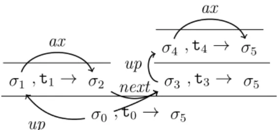
iii) rules 2, the rules with two inductive premises. Ax σ, t→ σ� R1 σ1, t1 → σ� 1 σ, t→ σ� R2 σ1, t1 → σ� 1 σ2, t2 → σ2� σ, t→ σ� FIGURE1.7 – Types of rules for a Pretty-Big-Step semantics
In Pretty-Big-Step, rules may take as input a memory and zero, one, or several values and they may either return a memory or a memory and also several value. To account for this in a uniform way, we define a state σ ∈ State as a pair of a memory and a list of values, called an extra. We write extra(σ) to refer to the list of values in a state σ. As often as possible, we will denote state with the letter σ (σ1, σ�, . . .) and memories with the letter M (M1, M�, . . .).
To simplify notations, if the extra is an empty list, we omit the extra and we only write the memory ; and if the extra is a singleton then we denote the state as a pair of a memory and the value in the extra.
A rule is entirely defined by the following components. — Axioms
— t : term, the term on which the axiom can be applied ;
— ax : State → State, a function that give the resulting state given the initial state.
— Rule 1
— t : term, the term on which the rule 1 can be applied ;
— t1 : term, a term to evaluate in order to continue the derivation ;
— up : State → State, a function that returns the new state in which t1
will be evaluated. — Rule 2
— t : term, the term on which the rule 2 can be applied ;
— t1, t2 : term, the terms to derive in order to get the result for t ;
— up : State → State, a function returning the state in which the term t1 has to be derived ;
— next : State ∗ State → State, a function giving the state in which t2
had to be derived depending on the initial state and the result of the derivation of t1.
σ1 , t1 → σ2 σ4 , t4 → σ5 σ3 , t3 → σ5 σ0 , t0 → σ5 ax ax up up next
The functions ax, up, and next are partial functions because the rules may not be defined for every state. For example, the rule IFTRUE above is defined
only when the state has a single extra that is the boolean value true.
Figure 1.8 shows again the three types of rules but with their explicit com-ponents. Ax σ, t→ ax(σ) R1 up(σ), t1 → σ � σ, t→ σ� R2 up(σ), t1 → σ � 1 next(σ, σ � 1), t2 → σ � σ, t→ σ�
FIGURE1.8 – Types of rules for a Pretty-Big-Step semantics (bis)
When describing a derivation σ, t → σ� (or a rule with this derivation as
conclusion), we will refer to σ as the semantic context of the derivation (or the rule) and to σ� as the result of the derivation (or the rule).
The intuition behind the Pretty-Big-Step rules is the following.
— If the evaluation is immediate, we can directly give the results (e.g., the evaluation of a skip statement or a constant). This behavior cor-responds to an axiom.
— If the evaluation needs to branch depending on a previously compu-ted value, stored as an extra, then a rule 1 is used for each possible branching. This is used for instance after evaluating the condition in a conditional statement.
— If the evaluation first needs to compute an intermediate result, then a rule 2 is used. The intermediate result is used to compute the next state with which the evaluation continues. This is how the conditional
statement works : first evaluate the guard and then compute another term in a state containing the result of the evaluation.
As an example, Figure 1.9 shows the derivation of the program
if x then0 else 1 in a state for which the stored value of x is true.
M, x→ (M, true)
M,0 → (M, 0)
(M, true), If1 (0) (1) → (M, 0)
M, if x then0 else 1 → (M, 0)
FIGURE 1.9 – Derivation of a simple program
1.3.2 Advantages
Modularity
The first advantage of Pretty-Big-Step is that it is very modular : extending the language can be done by adding new rules and without modifying previous ones. For instance, let us suppose we have a C-like for loop :
for(initialization, condition, step){body}
and see the differences in Big-Step and Pretty-Big-Step when adding the notion of errors. As shown in Figure 1.10, in Big-Step style, there are two rules to write to handle the for loop : one for each evaluation of the condition. In the first case, we start the loop by initializing, then we test for the condition, if the result is true we continue by evaluating the body, we proceed by doing the step for the next loop and finally we go back to the beginning of the loop ignoring the initialization phase. The second case also starts with the initialization and the evaluation of the condition, but if the evaluation returns false, the execution stops here.
FORTRUE
M0, init→ M1 M1, cond→ (M2, true) M2, body → M3
M3, step→ M4 M4, for(skip, cond, step){body} → M5
M0, for(init, cond, step){body} → M5
FORFALSE M0, init→ M1 M1, cond → (M2, f alse)
M0, for(init, cond, step){body} → M2
FIGURE1.10 – Rules of the for loop in Big-Step
Conversely, Figure 1.11 shows the 6 rules needed to handle the for loop in Pretty-Big-Step style. They introduce intermediate terms for1, for2 and for3.
They do not have the parameter init since these new terms corresponds to the loop phases.
FOR M, init→ σ σ, for1(cond, step){body} → σ �
M, for(init, cond, step){body} → σ�
FOR1 M, cond→ σ
σ, for2(cond, step){body} → σ� M, for1(cond, step){body} → σ
�
FOR2TRUE M, body → σ
σ, for3(cond, step){body} → σ� (M, true), for2(cond, step){body} → σ
�
FOR2FALSE
(M, f alse), for2(cond, step){body} → M
FOR3 M, step→ σ σ, for1(cond, step){body} → σ �
M, for3(cond, step){body} → σ
�
FIGURE1.11 – Rules of the for loop in Pretty-Big-Step
To derive the rule FOR, one needs to first evaluate the initialization init
and then for1 as the continuation. This first extended term is evaluated with
the rule FOR1 which evaluates the condition and then lets the term for2
decide to take the loop or not depending on the value calculated. The term for2 has then 2 ways to be evaluated : either the extra is true and in that
applies. In the first case, the program enters in the loop evaluating body and letting for3 taking care of ending the loop. In the second case there is no
computation left and the loop ends here. Once the body is executed, the rule FOR3 proceeds to evaluate the step statement and continues with the same
continuation as after the initialization : for1.
It is important to note that, despite the increasing number of rules, the number of inductive premises stays approximately the same : 7 premises in Big-Step and 8 in Pretty-Big-Step.
Let us extend the language with an error exception and commands to throw and catch this error and compare the changes to operate in Big-Step and in Pretty-Big-Step.
Error handling in Big-Step
In the Big-Step version, we suppose we have the rules of Figure 1.12 to throw and catch errors.
THROW M, throw→ (M, err) TRYCATCH M, body → (M � , err) M�, serror → σ �
M, try body catch serror → σ�
TRYNOCATCH M, body → σ �
σ� �= (M�, err) M, try body catch serror→ σ
�
FIGURE1.12 – Rules of throw and catch Big-Step style
To handle the interaction of errors with loops, one needs to add the 5 rules of Figure 1.13. Each rule corresponds to a step that could throw an error during the evaluation : the initialization, the condition, the body, the step and the next loops. We added 5 rules with a total of 15 premises.
Error handling in Pretty-Big-Step
In Pretty-Big-Step, it is way simpler because the structure allows to propagate the errors between each intermediate step thanks to the extra. First let us give the rules to throw and catch errors in Figure 1.14
FORERR1 M0, init→ (M1, err)
M0, for(init, cond, step){body} → (M1, err)
FORERR2 M0, init→ M1 M1, cond→ (M2, err)
M0, for(init, cond, step){body} → (M2, err)
FORERR3
M0, init→ M1
M1, cond→ (M2, true) M2, body → (M3, err)
M0, for(init, cond, step){body} → (M3, err)
FORERR4
M0, init→ M1 M1, cond→ (M2, true)
M2, body → M3 M3, step → (M4, err)
M0, for(init, cond, step){body} → (M4, err)
FORERR5
M0, init→ M1
M1, cond → (M2, true) M2, body → M3 M3, step → M4
M4, for(skip, cond, step){body} → (M5, err)
M0, for(init, cond, step){body} → (M5, err)
FIGURE1.13 – Extra rules about for/catch interaction (BS)
THROW
M, throw→ (M, err) TRY
M, body → σ σ, catch serror → σ� M, try body catch serror → σ
�
CATCH M, serror → σ �
(M, err), catch serror → σ �
NOCATCH lextra �= [err]
(M, lextra), catch serror → M
FIGURE1.14 – Rules of throw and catch Pretty-Big-Step style
Now to handle the interactions of errors with other terms, we need to add the rule of Figure 1.15 for every rule 2 over a term t and with t1 as term for
the first subderivation, excepted for the rule TRY.
In any rule 2, when an error occurs in the left branch, the rule ERR
ERR up(σ), t1 → (M, err)
σ, t→ (M, err)
FIGURE1.15 – Extra rules about for/catch interaction (PBS)
an error appears in the subderivation of a rule 1, the error is naturally trans-mitted to the result. In the case of the loop it corresponds to a total of 4 additional rules and only 4 premises.
On one hand, the adding of the new rules in Pretty-Big-Step is way simpler since it matches the total number of rules 2 whereas in Big-Step many rules need to be added to manage errors in a rule with more than two premises. On the other hand, the additional rules in PBS are fewer and smaller in terms of premises because there is no redundant subderivation in different rules.
Abstraction
The second advantage is that Pretty-Big-Step is really easy to abstract. Our formalization is stricter than Charguéraud initial version of Pretty-Big-Step. The extra part, which Charguéraud included in the subterm to evaluate, is now in the state. It allows to fully define each rule by a strict scheme depen-ding on which kind of rule it is (axiom, Rule1 or Rule2). We will see in Chapter 2 that we can work with a Pretty-Big-Step language without concretizing the terms of the language, only considering the structure of the rules. This is an important property since it allow any language to fit in our work at the only condition that it is written in Pretty-Big-Step form.
1.3.3 A While language in PBS
To illustrate our approach, we introduce a small WHILE language suitable for non-interference. It is a classical WHILE language with input/output com-mands to receive and send data. We first give the syntax of the language and then its semantics in Pretty-Big-Step form.
Memory model We propose to model non-interference by making explicit the inputs of a program and its outputs. We do not consider interactive
pro-grams, so each input is a constant single value, for instance an argument of the program. Outputs, however, consist of lists of values, as we allow a program to send several values to a given output.
Formally, we consider given a set of values Val, a set of variables Var, a set of inputs Inputs and a set of outputs Outputs. We define the memory as a triplet (Ei, Ex, Eo), where Ei ∈ Envi represents the inputs of a program
as a read-only mapping from each input to a value, Ex ∈ Envx represents
run-time environment as a read-write mapping from each variable to a value, and Eo ∈ Envorepresents the outputs of a program, as a write-only mapping
of each output to a list of values, accumulated in the output. To simplify, we consider inputs and outputs to be indexed by an integer.
Envi := Inputs �→ Val
Envx := Var �→ Val
Envo:= Outputs �→ List(Val)
Mem := Envi × Envx × Envo
Extra := List(Val) State := Mem × Extra
For the purpose of notation, when there is no ambiguity, memories and states may be seen has functions from Inputs, Var, or Outputs to Val or List(Val) to represent the part of the memory that should be used. For example, the value stored in the variable x in a memory M or a state σ may be written M(x) or σ(x).
Syntax In this language, we distinguish expressions and statements but they formally both are defined as terms. An expression is either a constant value, a variable, an input, or the addition of two expressions. A statement is either a no-op operation skip, a sequence of two statements, a conditional, a while loop, an assignment of an expression into a variable, or an assignment of an expression into an output.
�term� t : := Const n | Var x | Input i | Plus t t | Skip | Seq t t | If t t t | While t t | Assign x t | Output o t
We add to the language the extended terms required by the Pretty-Big-Step format.
�term� t : := . . . | Plus1 t | Plus2 | Seq1 t | If1 t t | While1 t t | While2 t t | Assign1 x | Output1 o
Semantics The difference between expressions and statements is at the semantic level where expressions always return a value, while statements may do so (the if statement for example) but it is not always the case.
To simplify the reading of the rules and the examples, we use some usual notations : cfor Const c xfor Var x e1+ e2 for Plus1 e2 +1e2 for Plus2 +2for Plus e1 e2 s1; s2 for Seq s1 s2 ;1s2 for Seq1 s2 x:= e for Assign x e x:=1for Assign1 x
if e then s1 else s2 for If e s1 s2
If1s1 s2 for If1 s1 s2
while e do s for While e s while1 e do s for While1 e s
while2 e do s for While2 e s
To evaluate a constant c the axiom CST requires the semantic context to
be a memory and an empty extra, and returns a result formed by the same memory and an extra containing the value c. The rule VAR looks up for the
value stored in x and returns a state made of the memory unmodified and the value found. The rule INPUTworks exactly the same way but in the input
environment.
The addition e1+ e2 of two expressions is managed by three rules PLUS,
PLUS1 and PLUS2. The first one is a rule 2 in which the first premise derives
the first expression e1 and the result of this derivation becomes the semantic
context of the second premise. This second premise is the derivation of +1e2
and requires the rule PLUS1. This rule is also a rule 2 : its first premise is
of the current rule (corresponding to the value of the first expression e1) is
added to the extra in the result of the derivation of e2 to form the semantic
context of the continuation. Finally, the axiom PLUS2 can add the two values
currently in the extra to produce the final sum.
To derive the skip, the rule SKIP needs a state with an empty extra and
returns the same state.
The sequence is derived with the rules SEQand SEQ1. The first rule is a
rule 2 that derives the first statement and passes the result to the continuation ;1. Then the second rule is a rule 1 simply deriving the second statement.
In the rule IF, the derivation of if e then s1 else s2 starts with the
deri-vation of the guarding condition e. The result is passed to the extended sta-tement If1 s1 s2. We then have two rules to evaluate If1 s1 s2, one for each
possible extra. The first one, IFTRUE, is a rule 1 in which the premise is the
derivation of the first branch granted that the value in the extra is true. The second one, IFFALSE, derives the second branch when the extra is false.
The rules to derive while e do s are similiar to those to derive an if sta-tement. First the rule WHILE derives the guarding condition. Then two cases
can appear. Either we have to derive while1 e do s in a state with an extra
containing false and in that case the axiom WHILEFALSE simply returns the
state without the extra. Or we have to derive the extended term in a state with truein the extra and then firstly the rule WHILETRUE1 derives the body of the
loop and lets the continuation while2 e do s decide the remaining derivations
to do, secondly the rule WHILETRUE2 branches back to the beginning of the
loop deriving again while e do s.
An assignment x := e is derived by the rule 2 ASG that derives the
ex-pression e and gives the result to the continuation x :=1. This extended term
can be derived by the rule ASG1 in an state containing a value v in the extra.
The resulting state is the same than the semantic context with v stored in x instead of the previous value.
The output Ouput o e of an expression e to an output o is similar : first the rule OUTPUT derives the expression to get its value and gives it to the
continuation, then the continuation is derived with the rule OUTPUT1 which
CST M, c → (M, c) VAR M(x) = v M, x→ (M, v) INPUT M(i) = v M, Input i → (M, v) PLUS M, e1 → (M � , v1) (M�, v1), +1e2 → (M��, v) M, e1+ e2 → (M��, v) PLUS1 M, e2 → (M � , v2) (M�,[v1, v2]), +2 → M �� , v (M, v1), +1e2 → M �� , v PLUS2 v = v1+ v2 (M, [v1, v2])), +2 → (M, v) SKIP M, skip → M SEQ M, s1 → M � M�,;1s2 → M �� M, s1; s2 → M �� SEQ1 M, s→ M� M,;1s → M � IF M, e→ (M � , v) (M�, v), If1s1 s2 → M �� M, if e then s1 else s2 → M�� IFTRUE M, s1 → M � (M, true), If1 s1 s2 → M� IFFALSE M, s2 → M � (M, f alse), If1 s1 s2 → M�
WHILE M, e→ (M � , v) (M�, v), while1 e do s→ M �� M, while e do s→ M�� WHILEFALSE (M, f alse), while1 e do s→ M WHILETRUE1 M, s→ M � M�, while2e do s→ M �� (M, true), while1 e do s→ M ��
WHILETRUE2 M, while e do s→ M � M, while2 e do s→ M � ASG M, e→ (M � , v) (M�, v), x :=1→ M �� M, x:= e → M�� ASG1 M� = M [x �→ v] (M, v), x :=1→ M � OUTPUT M, e→ (M � , v) (M�, v), Ouput1 o→ M �� M, Ouput o e→ M�� OUTPUT1 M � = M [o �→ v :: M (o)] (M, v), Ouput1 o→ M �
G
ENERIC FORMAT OF SEMANTICS
2.1 Motivation
As we stated before, we want our framework to work on a large variety of languages. The only constraints we enforce is that the languages semantics must be written in PBS form. It allows our framework to be independent of any language.
In order to be able to fit any PBS semantic in this work, we developed a formal PBS structure in which the three types of rules are formally defined. It gives the possibility to think of any language only in terms of axioms, rules 1 and rules 2 ; and to totally abstract the proofs from any particular language.
One other main reason to this choice is that JavaScript is widely used in browser and web application (which are uses for which non-interference makes sense to study) and already has a PBS semantics called JScert [13]. This semantics is a huge inductive definition with more than 800 rules and hinders formal proofs as Coq runs out of memory when performing an inver-sion or an induction.
Moreover, given a PBS semantic of any language in this formalism, we want to automatically derive the associated multisemantics that we will build in section 3.
2.2 Formal Pretty-Big-Step
2.2.1 Abstract PBS
We first define what a syntax is. It simply consists of terms and values. Such a syntax can be assumed by the use of type classes.
Class AbstractSyntax := {
Term : Type;
Value : Type
}.
Context {Syntax : AbstractSyntax}.
Now that we have some terms and values, we can define variables as strings and then describe our memory model as in subsection 1.3.3. A State is made of 4 parts : a memory for the inputs, one for the variables, a last one for the outputs, and the extra.
Definition variable : Type := string.
Definition input : Type := string.
Definition output : Type := string.
Record State :=
mkState
{
Envi : input -> Value; (* input environment *)
Envx : variable -> option value; (* variable environment *)
Envo : output -> list value; (* output environment *)
extra : list value (* extra *) }
.
Once the memory model is defined, we have the ability to formally define the PBS rules. There are three kinds of rules :
1. To entirely define an axiom, we exactly need the term t on which it applies and the function ax returning the resulting state ; for the purpose of capturing non-interference by the multisemantics we also add four sets and a boolean value : 2 sets for the inputs and variables read by the axiom, 2 sets for the variables and outputs written by the axiom and a boolean value to specify if the axiom produces an extra or if it returns an empty one. These parameters are not mandatory for a PBS but they will be used and explained in a more detailed way in chapter 4.
2. A Rule 1 is defined by the term t on which it applies, the term t1 needed
to derive, and the function up returning the semantic context in which t1
must be derived.
3. And a Rule 2 is defined by the term t on which it applies, the terms t1
and t2 that need to be derived, the function up returning the semantic
context in which t1 must be derived and the function next returning the
semantic context in which t2 must be derived.
Inductive rule :=
| Ax : Term (*t*)
-> (State -> option State) (*ax*)
-> fset input (*Inputs read*) -> fset variable (*Variables read*) -> fset variable (*Variables written*) -> fset output (*Outputs written*)
-> bool (*extra produced*)
-> rule
| R1 : Term (*t*)
-> Term (*t1*)
-> (State -> option State) (*up*) -> rule
| R2 : Term (*t*)
-> Term (*t1*)
-> Term (*t2*)
-> (State -> option State) (*up*) -> (State -> State -> option State) (*next*) -> rule
.
Now that we gave a structure to our rule format we can formally define a semantics, i.e. a function giving, for each term, a list of rules that can be applied to the term. As for syntax, let us assume we have a semantics.
Class AbstractSemantics := {
}.
Context {Semantics : AbstractSemantics}.
The definition of a derivation is now possible. A derivation of term t from the semantic context σ to the result out is defined inductively with these 3 cases :
Inductive deriv (t:Term) (sigma:State) (out:State) : Prop :=
1. if there is axiom R in the semantics such that ax(σ) = Some out
| deriv_Ax R ax ri rx wx wo pe
(eqR : R = Ax t ax ri rx wx wo pe) (isRule : List.In R (Rules t)) (eqAx : ax sigma = Some out) : (* ======== *)
deriv t sigma out
2. if there is a rule 1 R in the semantics and a state σ1, such that up(σ) =
Some σ1 and there is a derivation of t1 from σ1 to out. | deriv_R1 R t1 up sigma1
(eqR : R = R1 t t1 up)
(isRule : List.In R (Rules t)) (eqUp : up sigma = Some sigma1) (STEP : deriv t1 sigma1 out) : (* ======== *)
deriv t sigma out
3. if there is a rule 2 R in the semantics and three states σ�, out� and σ��
such that up(σ) = Some σ�, there is a derivation of t
1 from σ� to out�,
next(σ, out�) = Some σ��and there is a derivation of t2 from σ��to out. | deriv_R2 R t1 t2 up next sigma’ out’ sigma’’
(eqR : R = R2 t t1 t2 up next) (isRule : List.In R (Rules t)) (eqUp : up sigma = Some sigma’) (STEP1 : deriv t1 sigma’ out’)
(STEP2 : deriv t2 sigma’’ out) : (* ======== *)
deriv t sigma out
.
2.2.2 Concretization of the WHILE language
To illustrate a concretization of a pbs language, we formalize the while language described in subsection 1.3.3. Values and Terms are defined in-ductively. Values are either integer or boolean.
Inductive Concr_value : Type := | Num (z:Z)
| Bool (b:bool) .
Inductive Concr_Term: Type := (*Statements*)
| Skip : Concr_Term
| Seq : Concr_Term -> Concr_Term -> Concr_Term
| Seq1 : Concr_Term -> Concr_Term
| If : Concr_Term -> Concr_Term -> Concr_Term -> Concr_Term
| If1 : Concr_Term -> Concr_Term -> Concr_Term
| While : Concr_Term -> Concr_Term -> Concr_Term
| While1 : Concr_Term -> Concr_Term -> Concr_Term
| While2 : Concr_Term -> Concr_Term -> Concr_Term
| Assign : variable -> Concr_Term -> Concr_Term
| Assign1 : variable -> Concr_Term
| Out : output -> Concr_Term -> Concr_Term
| Out1 : output -> Concr_Term
(*Expressions*)
| Var : variable -> Concr_Term
| Cons : Concr_value -> Concr_Term
| Plus1 : Concr_Term -> Concr_Term
| Plus2 : Concr_Term
| In : input -> Concr_Term
.
These values and terms form our syntax :
Instance Concr_Syntax : AbstractSyntax:= {
Value := Concr_value;
Term := Concr_Term
}.
We only describe here the rules for the Skip, If, Out, Var, Plus and In terms. The complete Coq code can be found in Appendix A. The appendix also shows 3 functions to change the extra of a state (update_extra), to modify the value of a variable (update_var) or an output (update_output). The rules are given by a function returning, for each term, a list of rules that can be applied to it.
Definition Concr_Rules (t:Concr_Term): list rule :=
match t with
The only rule for the term Skip is an axiom : the term it applies on is of course Skip. The ax function is a partial function defined only if the extra is empty : if it is empty, ax returns the semantic context as the result and if it is not ax returns None to illustrate that there is no possible derivation. All of the sets are empty since the rule does not read or write any input, variable or output. Additionally, this rule does not produce an extra therefore the boolean value is false.
| Skip => (Ax Skip
(fun sc => match extra sc with
| nil => Some sc
| _ => None end)
empty empty empty empty
false) :: nil
The term If e s_1 s_2 cannot be directly derived with an axiom and needs other derivations. The rule for the if statement is a rule 2 in which the first term to derive is the guard e and the second one is the extended term if1 s1 s2. The partial function up is defined only if the extra of the
seman-tic context is empty and in that case, it returns the same semanseman-tic context for the guard. On the other hand, next is defined only if up is defined and if the extra of the first derivation’s result is a singleton containing a boolean value. In that case next returns the result of the first derivation as semantic context for the If1 statement. Note that this mechanism allows the presence of side
effects to the memory during the derivation of the guard.
| If e s1 s2 => (R2 (If e s1 s2) (e)
(If1 s1 s2)
(fun sc => match extra sc with
| nil => Some sc
| _ => None end)
(fun sc res => match extra sc, extra res with
| nil, (Bool _) :: nil => Some res
| _,_ => None end)) :: nil
Once the guard has been evaluated and stored in the extra, the term if1 s1 s2 can be derived in two possible ways depending on the value stored.
Therefore, there are two rules for this term. Both rules are rule 1 and they can only be applied when the extra of the semantic context contains nothing more than a boolean value. If the boolean is true, the first rule applies and it considers s1 for the inductive derivation. In the other case, the second rule
applies and it considers s2. Both up functions keep the memories unchanged
and replace the extra by an empty list.
| If1 s1 s2 => (R1 (If1 s1 s2) (s1)
(fun sc => (match extra sc with
| (Bool true) :: nil =>
| _ => None end))) ::
(R1 (If1 s1 s2) (s2)
(fun sc => (match extra sc with
| (Bool false) :: nil =>
Some (update_extra sc nil) | _ => None end)))
:: nil
To output an expression e on o, a rule 2 applies : first derive e and then Out1o. The up partial function requires an empty extra in the semantic context
and returns the same state. The next function additionally requires that the extra of the first derivation’s result is a singleton and returns the result of the first derivation.
| Out o e=> (R2 (Out o e) (e)
(Out1 o)
(fun sc => match extra sc with
| nil => Some sc
| _ => None end)
(fun sc res => match extra sc, extra res with
| nil, v :: nil => Some res
| _,_ => None end)) :: nil
Then to derive the extended term Out1 othe rule to apply is the following
axiom. The ax partial function is defined provided that the extra in the seman-tic context contains only one value v and it returns the same state but with v added to the output o and an empty extra. In that case, the axiom does not read any input or variable and neither it writes into a variable ; but it writes into the output o thus the fourth set is the singleton {o}. Since this axiom only sends the value in the output o, it does not produce a value in the extra. therefore the boolean value is set to false.