The California Current System: A multiscale overview and the development of a feature-oriented regional modeling system (FORMS)

The California Current System: A multiscale

overview and the development of a

feature-oriented regional modeling system (FORMS)

Citation Gangopadhyay, Avijit; Lermusiaux, Pierre F.J.; Rosenfeld, Leslie; Robinson, Allan R.; Calado, Leandro; Kim, Hyun Sook; Leslie, Wayne G. and Haley, Patrick J.“The California Current System: A Multiscale Overview and the Development of a Feature-Oriented Regional Modeling System (FORMS).” Dynamics of Atmospheres and Oceans 52, no. 1–2 (September 2011): 131–169 © 2011 Elsevier B.V.

As Published http://dx.doi.org/10.1016/j.dynatmoce.2011.04.003

Publisher Elsevier

Version Original manuscript

Citable link http://hdl.handle.net/1721.1/110434

Terms of Use Creative Commons Attribution-NonCommercial-NoDerivs License

The California Current System: A Multiscale Overview and the Development

of a Feature-Oriented Regional Modeling System (FORMS)

Avijit Gangopadhyay

School for Marine Science and Technology, University of Massachusetts at Dartmouth, MA

P.F.J. Lermusiaux

Department of Mechanical Engineering, Massachusetts Institute of Technology, Cambridge, MA

Leslie Rosenfeld

Naval Postgraduate School, Monterey, CA

A.R. Robinson

Division of Applied Sciences, Harvard University, Cambridge, MA

Leandro Calado Marinha do Brasil

Instituto de Estudos do Mar Almirante Paulo Moreira - IEAPM Rua Kioto, 253 - Praia dos Anjos, Arraial do Cabo, RJ – Brasil 28930-000

H.S.Kim

National Center for Environmental Prediction (NCEP), Silver Springs, MD

W.G. Leslie, P.J. Haley, Jr.

Department of Mechanical Engineering, Massachusetts Institute of Technology, Cambridge, MA

Submitted to Dynamics of Atmospheres and Oceans

*Corresponding author. Dr. Avijit Gangopadhyay, SMAST, University of Massachusetts Dartmouth, Suite 325, 200 Mill Road, Fairhaven, MA 02719.

Telephone: (508) 910-6330 Fax: (508) 910-6374; E-mail: [email protected]

Manuscript

Report Documentation Page OMB No. 0704-0188Form Approved

Public reporting burden for the collection of information is estimated to average 1 hour per response, including the time for reviewing instructions, searching existing data sources, gathering and maintaining the data needed, and completing and reviewing the collection of information. Send comments regarding this burden estimate or any other aspect of this collection of information, including suggestions for reducing this burden, to Washington Headquarters Services, Directorate for Information Operations and Reports, 1215 Jefferson Davis Highway, Suite 1204, Arlington VA 22202-4302. Respondents should be aware that notwithstanding any other provision of law, no person shall be subject to a penalty for failing to comply with a collection of information if it does not display a currently valid OMB control number.

1. REPORT DATE

2010 2. REPORT TYPE

3. DATES COVERED

00-00-2010 to 00-00-2010

4. TITLE AND SUBTITLE

The California Current System: A Multiscale Overview and the

Development of a Feature-Oriented Regional Modeling System (FORMS)

5a. CONTRACT NUMBER 5b. GRANT NUMBER

5c. PROGRAM ELEMENT NUMBER

6. AUTHOR(S) 5d. PROJECT NUMBER

5e. TASK NUMBER 5f. WORK UNIT NUMBER 7. PERFORMING ORGANIZATION NAME(S) AND ADDRESS(ES)

Naval Postgraduate School,Monterey,CA,93943

8. PERFORMING ORGANIZATION REPORT NUMBER

9. SPONSORING/MONITORING AGENCY NAME(S) AND ADDRESS(ES) 10. SPONSOR/MONITOR’S ACRONYM(S) 11. SPONSOR/MONITOR’S REPORT NUMBER(S)

12. DISTRIBUTION/AVAILABILITY STATEMENT

Approved for public release; distribution unlimited

13. SUPPLEMENTARY NOTES

14. ABSTRACT

Every littoral or regional ocean has both coastal circulation components and influences from offshore regions. Over the past decade, the feature-oriented regional modeling approach has evolved to become operational in some of these regions (western North Atlantic, tropical North Atlantic). This methodology is model-independent and can be applied with or without satellite and/or in situ observations, especially in coastal regions. In applying this methodology for the subtropical North Pacific, we first present an overview of the synoptic nature of the different features that comprise the multiscale and complex

circulation in the California Current system (CCS). This description is a prerequisite to feature modeling and is based on our present understanding of the features and their dominant space and time scales of variability. The region of interest is from 36?N to 48?N ? essentially most of the eastern boundary current region of the subtropical North Pacific. We present a synergistic configuration of synoptic features

interacting with one another on multiple and sometimes overlapping space and time scales as a

meandereddy- upwelling system. The second step is to define the feature-oriented regional modeling system (FORMS) for this system. The major multiscale synoptic circulation features include the mean flow and southeastward meandering jet(s) of the California Current, the poleward flowing California Undercurrent, and six upwelling regions along the western coast of the U.S. We first identify the typical synoptic width, location, vertical extent, and core characteristics of these features and their dominant spatial and temporal scales of variability from past observational theoretical and modeling studies. These synoptic features are then melded with available climatology of the region for initialization and assimilation. Finally, dynamical simulations are run as nowcasts and short-term (4-6 weeks) forecasts using these feature models as initial fields and the Princeton Ocean Model (POM) for dynamics. The set of simulations over a 40-day period illustrate the applicability of FORMS to a transient eastern boundary current region such as the CCS. The success of the dynamical simulations were realized in (i) maintenance of the low-salinity pool in the core of the CC; (ii) representation of eddy activity inshore of the coastal transition zone; (iii) realistic eddy kinetic energy evolution (iv) subsurface (intermediate depth) mesoscale feature evolution; and (v) deep poleward flow evolution.

15. SUBJECT TERMS

16. SECURITY CLASSIFICATION OF: 17. LIMITATION OF ABSTRACT Same as Report (SAR) 18. NUMBER OF PAGES 63 19a. NAME OF RESPONSIBLE PERSON a. REPORT unclassified b. ABSTRACT unclassified c. THIS PAGE unclassified

Standard Form 298 (Rev. 8-98) Prescribed by ANSI Std Z39-18

Abstract

Every littoral or regional ocean has both coastal circulation components and influences from offshore regions. Over the past decade, the feature-oriented regional modeling approach has evolved to become operational in some of these regions (western North Atlantic, tropical North Atlantic). This methodology is model-independent and can be applied with or without satellite and/or in situ observations, especially in coastal regions. In applying this methodology for the subtropical North Pacific, we first present an overview of the synoptic nature of the different features that comprise the multiscale and complex circulation in the California Current system (CCS). This description is a prerequisite to feature modeling and is based on our present understanding of the features and their dominant space and time scales of variability. The region of interest is from 36°N to 48°N – essentially most of the eastern boundary current region of the subtropical North Pacific. We present a synergistic configuration of synoptic features interacting with one another on multiple and sometimes overlapping space and time scales as a meander-eddy-upwelling system. The second step is to define the feature-oriented regional modeling system (FORMS) for this system. The major multiscale synoptic circulation features include the mean flow and southeastward meandering jet(s) of the California Current, the poleward flowing California Undercurrent, and six upwelling regions along the western coast of the U.S. We first identify the typical synoptic width, location, vertical extent, and core characteristics of these features and their dominant spatial and temporal scales of variability from past observational, theoretical and modeling studies. These synoptic features are then melded with available climatology of the region for initialization and assimilation.

The set of simulations over a 40-day period illustrate the applicability of FORMS to a transient eastern boundary current region such as the CCS. The success of the dynamical simulations were realized in (i) maintenance of the low-salinity pool in the core of the CC; (ii) representation of eddy activity inshore of the coastal transition zone; (iii) realistic eddy kinetic energy evolution; (iv) subsurface (intermediate depth) mesoscale feature evolution; and (v) deep poleward flow evolution. (Keywords: California Current System; Feature Models; FORMS; Upwelling)

1.

Introduction

The California Current system (CCS) is at the eastern boundary of the wind-driven subtropical gyre in the North Pacific. The region of interest for this multiscale (in space and time) overview is from 36°N to 48°N and from 145°W to the North American west coast. In short, large-scale gyres and mean southeastward flow are prevalent in climatological averages, while mesoscale eddies and submesoscale filaments are abundant in its synoptic state and are transient in nature. The regional ecosystem is well known for its productivity and the seasonal and inter-annual variability resulting from large-scale wind-driven upwelling around its multiple capes and their interactions with the irregular occurrences of the El Niňo – La Niňa phenomenon. The typical summer circulation is drastically different from that in the winter, and a synoptic description at any one time has been a challenge.

This region has been studied systematically from the early 1950s by the CALCOFI (California Cooperative Oceanic Fisheries Investigation; Wyllie, 1966) monitoring program. However, as in many other regions, the richness of mesoscale variability was recognized first in satellite SST images for this region, and then in color images now available from MODIS and other satellite sensors. Figure 1 shows the difference in features, their appearance, and prevalent scales as available from an SST image from those of a typical climatology. Clearly, the

averaging of data at larger scales masks the presence of many of the important mesoscale and submesoscale features of circulation.

This region of interest -- i.e., the western coast of the U.S. -- includes both a larger-scale dynamic offshore region and a finer-scale dynamic coastal region. The offshore region is

primarily dominated by the large-scale California Current, the California Undercurrent and parts of subtropical and sub-polar gyre circulations in the eastern Pacific. The coastal region includes features such as upwelling fronts, cold pools inshore of these fronts, filaments, squirts,

mushroom-head vortices, mesoscale and sub-mesoscale eddies, and meanders.

One of the approaches for regional modeling of such regions in the world oceans is the use of ―knowledge-based feature models.‖ This approach is distinctly different from the basin-scale approach that requires models to develop the inertia fields in a so-called ``spin-up'' period, which could be anywhere from one to ten years. Our goal is to develop a system for short-term synoptic forecasting for use where we cannot afford to run models for a long period of time for spin-up or if model biases could build up when numerical codes are run for long periods. This feature-oriented approach has been used for regional simulations and operational forecasting for the past two decades. It originated and was very successful in weather prediction when sufficient data were not available for a complete initialization of features (e.g. Bennett, 1992; Bennett, 2002). In the ocean, specific examples include the studies by Robinson et al. (1989), Hurlburt et

al. (1990, 1996), Fox et al. (1992), Glenn and Robinson (1995), Cummings et al. (1997),

Gangopadhyay et al. (1997), Lermusiaux (1999a), and Robinson and Glenn (1999) that have applied the feature modeling technique for use in nowcasting, forecasting and assimilation of various in situ (XBT, CTD) and satellite (SST, SSH [GEOSAT, TOPEX/Poseidon] and SSC

Gangopadhyay and Robinson (2002) have generalized the feature-oriented approach for strategic application to any regional ocean. A feature-oriented regional modeling system

(FORMS) for the Gulf of Maine and Georges Bank region has been developed for real-time applications for medium-range (7-10 days) and mesoscale to sub-mesoscale forecasting (Gangopadhyay et al., 2003; Brown et al. 2007a,b). This feature-oriented methodology is also model-independent and can be applied in lieu of either satellite or in situ observations, or both, especially in coastal regions. It has been applied in many real-time simulations, including the recent IOOS efforts (Schofield et al, 2010).

Feature-oriented methodology requires developing a synoptic circulation template for the region, called the ―basis template.‖ This template is designed from a feature-based synthesis of the regional circulation patterns. From this ―basis template,‖ a map of strategic sampling locations for placing feature model profiles is produced. These profiles provide ―synthetic synoptic expressions‖ for fronts, jets, eddies, gyres, and other circulation structures and water masses at the initialization or updating phases. Features are represented by both analytical structures and by synoptic sections and profiles. The feature model profiles for a typical feature are developed by analyzing past synoptic high-resolution observations for that feature.

Gangopadhyay and Robinson (2002) described the generalized mathematical forms for some of the typical feature models developed so far (see their Appendix A). Gangopadhyay et al. (2003) described a number of applications for coastal regions such as a coastal current, a tidal mixing front, eddies and gyres.

For any oceanic region such as the California Current system, such structures and parameterized forms can be implemented to characterize the relevant circulation entities. Such implementation requires careful and detailed scientific analyses to identify the spatial and

temporal scales and variability that define and distinguish these features from one another while preserving the particular characteristics and dynamic balances of each feature. After major features are identified and individually represented, they are used in the initialization of a basic dynamical model (e.g., POM). Dynamical adjustment accomplishes two important tasks: i) a consistent dynamical interaction of the features, and ii) the generation of smaller-scale features, such as squirts and sub-mesoscale eddies.

In this study, we build on the experience and knowledge from the above studies to develop FORMS for the California Current system. The application of FORMS for nowcasting and forecasting is of interest to the US Navy, CeNCOOS, SCCOOS and similar entities. In Section 2, we first provide an overview of the synopticity of the CCS circulation. In Section 3, we then present a synopsis of the CCS features and their variability, which is the prerequisite first step of a feature-oriented regional modeling perspective. The individual feature models are described in Section 4. The FORMS protocol for initialization for this region is then illustrated in Section 5. Dynamical simulations using climatology and selected feature models are discussed in Section 6. Section 7 summarizes the results, and also outlines the future directions for

maintaining longer-term synoptic forecasts.

2.

A Brief Overview of the Synoptic Nature of the CCS

Moores and Robinson (1984) first described the instantaneous California Current (CC) as an energetic meandering jet, interacting with mesoscale eddies and coastal upwelling regions. During the OPTOMA (Ocean Prediction through Observation, Modeling and Analysis) exercises in the summers of 1983 and 1984, Robinson et al. (1984, 1986) designed the first, real-time

dynamical forecasting experiment in the CCS region and found that the time-scales of eddy-meander/ eddy-eddy interactions are on the order of 1-2 weeks in this region.

Brink et al. (1991) defined a coastal transition zone (CTZ) along the California coast as the demarcation between the faster, more energetic, shallow and narrow coastal upwelling-dominated flow system and the large-scale, broad mean southward flow in the deep offshore region. The transition zone was thought to be an area where mesoscale eddies and filaments would dominate. Strub et al. (1991) proposed a synoptic strong surface jet as the CC core meandering through a field of associated cyclonic and anticyclonic eddies. They also found evidence of some subsurface eddies which had no identifiable surface signatures. Hickey (1998) provided an end-of-the-century overview of the CCS, its seasonality and inter-annual variability. Hickey identified the core of the current as a freshwater signature, different from the coastal upwelling water masses.

A compilation of the physical, chemical and biological studies of the CCS in the past century was organized by Chavez and Collins (2000) in a special issue of DEEP SEA

RESEARCH. The mean structure of the poleward California Undercurrent (CUC) was described by Collins et al. (2000) along Pt. Sur. Pierce et al. (2000) showed the existence and continuation of this flow along the California coast, while Noble and Ramp (2000) analyzed the spatial and temporal variability in the CUC. The latter study showed how and where the poleward flow is surface-intensified and how the variability is related to the surface wind stress. Barth et al. (2000) described how the surface upwelling jets separate from the cape-like coast and become a conduit for transferring fluxes across the shelf.

Strub and James (2000) investigated the seasonality of the mesoscale evolution of the CCS based on altimeter-derived surface velocity fields. Eddy statistics such as eddy kinetic

energy (EKE), wavelengths of meanders and jets and their spatial extents were, for the first time, quantified. Strub and James (2000) raised two very important questions: one related to the formation and westward migration of the seasonal jet and another related to the source of freshwater within the CC core. They hypothesized that the seasonal jet begins as one or more local upwelling-front jets which move offshore by Rossby waves. These jets unite offshore (to about 130W) to become a free, open-ocean jet that maintains its identity as the CC core during spring and summer. Based on previous observation and models, Strub and James (2000) also hypothesized that the source of the fresh water in the core of the CCS has multiple contributions from the North Pacific Current, coastal inputs from the Columbia River, the Strait of Juan da Fuca and the British Columbia coast (sub-arctic origin).

In a high-resolution analysis of hydrographic data along line 67 during 1988-2002, Collins et al. (2003) observed the California Current jet at about 100-200 km offshore near Monterey Bay. Their analysis suggests that the ―mean‖ CC jet is at the inshore edge of the broader mean seasonal equatorward flow of the California Current. The mean jet's maximum velocity (6-10 cm/sec) is much weaker than that of the baroclinic jet (50-100 cm/sec) identified by Brink et al. (1991). One interpretation is that the average currents over the 50 km or so mean CC jet width are on the order of 10 cm/sec, but that much higher velocities are found in the narrow frontal regions within the CCS (Chavez, personal communication).

More recently, Belkin et al. (2009) carried out a frontal mapping characterization of the CCS based on available SST. Their frontal mapping for July 1985 and December 1985 (see their Figure 14) showed a dramatic change of scale (an order of magnitude) from summer to winter. The near-chaotic (disorganized and almost homogeneous) distribution of fronts in the summer

winter. This pattern is also observed in other eastern boundary current regions and is indicative of the prevalence of transitional and short-lived fronts associated with swift dynamical processes with time-scales of 1-10 days. This idea supports the Mooers and Robinson (1984) construct of meandering jets and filaments interacting with eddies and upwelling regions forced by short-period atmospheric winds. A more recent overview of the processes in the California Current System is presented by Barth and Chekley (2009).

Modeling and assimilation in the larger California Current region for understanding the complex processes have been a major focus of many investigators, including McWilliams et al. (1985), Miller et al. (1999), Mercheseilo et al. (2003), Penven et al. (2006), Caput et al. (2008 a,b), Moore et al. (2009) and others listed in these papers. During 2003 and 2006, major experiments occurred in the coastal region of Monterey Bay (around the middle of our coastal zone), revealing some of the faster upwelling dynamics processes and their interactions with larger-scale features including offshore eddies, the CUC and coastal trapped waves (e.g. Ramp et al, 2008; Chao et al, 2008; Haley et al, 2009; Shulman et al, 2009; Ramp et al, 2010- this-issue). It is clear from the above overview that this region is dynamically complex and rich with short-term energetic phenomena. Thus it is important to (i) develop a synoptic description of the system elements and (ii) characterize and document the scales and variability for possible use in modeling, initializing, validating and assimilating in a numerical prediction system.

3. Features, Scales and Variability in the CCS

Based on the above overview, we identified the following key points to be considered for a synoptic synthesis of features: (i) a synoptic state that can sustain a frontal jet of higher

these southward-flowing synoptic coastal jets mixing with the mean equatorward flow system (which is part of the large-scale subtropical gyre); (iii) offshore of Monterey Bay at around 37.5N, the synoptic jet (of Strub et al., 1991) and the mean current (of Collins et al., 2003) are within one degree of each other; (iv) the addition of a number of eddies might provide a more stable configuration.

We present below various aspects of the synoptic variability of the prevalent circulation features in the CCS, focusing on the summer (July-August) season. Some of these features can be seen in Figure 3 of Strub et al. (1991) which depicts surface pigment concentration from the CZCS satellite data from June 15, 1981. The characteristic CCS surface features can be seen in similar SST and color images (Strub and James, 2000). The features that we study and

characterize are: (i) the California Current (mean and its core jets); (ii) the California

Undercurrent; (iii) the Inshore Countercurrent (Davidson Current); (iv) the coastal transition zone that separates the shelf circulation from the offshore flows; (v) the eddies; (vi) the anomalous pools; (vii) the baroclinic jets along upwelling fronts; (viii) the filaments; (ix) the squirts and (x) the mushroom heads.

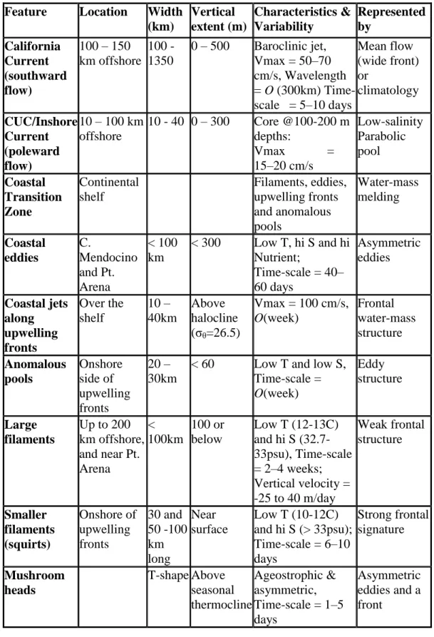
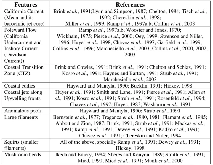
In particular, we provide a comprehensive synthesis of the typical synoptic widths, locations (distance from the coast), vertical extents, and core characteristics of these features. The dominant spatial and temporal scales of variability of each of these features are identified from past observational, theoretical and modeling analyses. They are indicated in Table 1. We discuss some of these features.

3.1 The California Current

surface. This frontal jet also meanders and develops eddies as it progresses southward and interacts with the onshore upwelling regions and their filaments. The low salinity core was probably first described by Lynn and Simpson (1987). They defined three cross-shore zones based on seasonal signal in dynamic height field from the CALCOFI data. Minimum in the dynamic height field was obtained in the winter in the offshore region due to cooling. Maximum in the dynamic height was observed in the winter caused by currents. Eddies dominated the transition zone in between, where the standard deviation of the dynamic height was high,

although its seasonal signal was relatively small. The core of the CC lies in this band. This is also consistent with the Strub et al. (1991) description of the jet flowing through the field of eddies (See Fig. 15 of LS87).

A synergistic set of three simple model alternatives for the flow structure of cold filaments proposed by Strub et al. (1991) (their Figure 1) is shown here in Figure 2. They proposed that the idealized squirt is generated by nearshore convergences, such as those caused by local wind relaxations around capes, so the squirts have an onshore energy source.

Alternatively, the field of mesoscale eddies could draw recently upwelled water away from the coast, which is an offshore energy source. The third alternative was to imagine a continuous southward jet meandering offshore and onshore. This jet may entrain coastally upwelled water and pull it offshore. While all of the preceding hypotheses may contribute to squirt formation, the last hypothesis of the meander-eddy-upwelling is becoming the prevailing view of the CCS in spring/summer (see also Ramp et al., 2009, Pringle and Dever, 2009).

In a larger context, the meander-eddy-upwelling system as initially proposed by Mooers and Robinson (1984) and adapted here in Figure 3 as a synoptic basis for synthesis of multiscale elements should be able to reproduce realistic jets, eddies and squirts in a dynamical modeling

framework. The schematic in Figure 3 shows the complexity in the meander-eddy-upwelling system of the California Current off Oregon and California in the spring/summer. The coastal jet coming from the north moves offshore as the season progresses (denoted by the March, May, and July lines), and contributes downstream to the low-salinity core of the California Current. This core delineates the higher variability region nearshore from the less active regions offshore. The offshore region consists of the mean southeastward flow of the wind-driven subtropical gyre. The inshore region is populated by upwelling centers concentrated near the capes. Eddies generated by the meandering jet are found in both regions, and may exhibit either cyclonic or anticyclonic rotation. Temporally transient eddies of various sizes have been observed.

3.2 The California Undercurrent (CUC)

The availability of synoptic data for the CUC is sparse. Differences in periods of analysis, geographical coverage, and lack of high-resolution synoptic surveys are the challenges of

pinpointing the location and behavior of this feature. Notably, Collins et al. (1996) showed that the path of the CUC during summer 1993 was close to the continental slope between San Francisco (37.8N) and St. George Reef (41.8N). Pierce et al. (2000) analyzed in detail a follow-up survey of 105 shipboard ADCP velocity sections during July to August 1995. They found that, on monthly average, the CUC has a core speed of >10 cm/sec between 200-275 m depth at 20-25 km off the shelf break. These sections and the core path are available from the website http://diana.oce.orst.edu.

3.3 The Coastal Upwelling Regions

Seasonal variations in the wind direction provides for different regimes along the coast of California. From March through September, prevailing northwesterly winds combined with the effect of the earth‘s rotation, drive surface waters offshore, leading to consistent upwelling region around the many capes (e.g. Fratantoni and Haddock, 2009). These deep, cold nutrient-rich waters are responsible for high productivity of California‘s near-shore region (DSR v53, 25-26, 2006). The upwelling activity subsides in September, when the northwesterlies die down, which leads to downwelling in October. The relaxation of the upwelling in August is described by Ramp et al. (2005) and in Rosenfeld et al. (1994). Haley et al. (2009) reported

four-dimensional simulation studies of dynamical processes in the Monterey Region, while Ramp et

al. (2010) compare different simulations of such dynamics, pointing to the importance of model

resolution and of longer coastal waves. The wintertime change in the atmospheric pressure leads to southwesterlies along the coast. The response along the coast is generally seen as a northward flow reversal at the surface, called the Inshore countercurrent, or the Davidson Current.

The inshore region of the CTZ is complicated by the poleward flow being interrupted by the summer upwelling jets flowing equatorward near the mouth of Monterey Bay (Collins et al., 2003). The water-mass characteristics of the Monterey Bay during the upwelling and relaxation periods were described in detail by Warn-Varnas et al. (2007). For the development of the FORMS for the CCS region during summer, we focus our study to the six upwelling regions around the six capes: Cape Blanco, Cape Mendocino, Pt. Arena, Pt. Reyes, Pt. Año Nuevo and Pt. Sur.

3.4 Other Mesoscale Features in the CCS Region

According to Collins et al. (2003), during fall and winter, when the upwelling is not present, the Inshore Countercurrent (Davidson Current) has two distinct cores, one on the coast and one 50 km offshore. Since our focus is on the development of CCS-FORMS for the

summertime, we defer to the development of this feature. Apart from these three currents, there are very energetic and important shallow water features in the CTZ around the coastal region of Monterey Bay and the California Current System. The filaments, coastal eddies, anomalous pools, jets along the upwelling fronts and mushroom-like vortices are critical to reproduce for accurate forecasting. The scales and variability of these features have been identified in Table 1, with relevant references cited in Table 2.

These features such as filaments, jets, and mushroom-vortices are related to specific dynamical processes, including instability, upwelling and wind-driving. It has been proposed by Brink et al. (1991) that subduction plays a very important role inside the filaments, forcing these cold filaments downwards, below the ambient warm surface waters. The mushroom vortices are generated only if certain conditions of the flow field are met (Mied et al., 1991).

For this first implementation of FORMS for the CCS, we have excluded such complications. However, as will be shown later, once the primary features are in place, the ensuing model integration generates mesoscale and submesoscale features such as filaments and mushroom vortices. Examples of such realistic simulations were given recently for the

4.

Feature Models for Different Features in the CCS

A prerequisite synthesis of the prevalent features in the CCS was presented in Section 3 and their spatial and temporal scales are summarized in Table 1. In particular, we have

investigated the typical synoptic width, location (distance from the coast), vertical extent, and core characteristics of these features. For the CCS-FORMS, we restrict ourselves to a

combination of the CC, CUC and upwelling feature models in a climatological background for initialization. Eddies can be added in a synoptic forecasting system, and multiple examples of such eddy feature models can be found in the studies by Gangopadhyay and Robinson (2002), Calado et al. (2006), Calado et al. (2008) and others. In this section we present the feature models that were developed based on previous synoptic studies for a subset of those features for this first application to numerical modeling.

4.1 Feature Models for the California Current and its Low Salinity Core

The schematic in Figure 3 shows the setup of different features in the CCS region. From a synoptic viewpoint, the California Current mean flow has a meandering jet structure at its core. We chose the low-salinity pool in the core of the CC as the primary characteristic and developed a feature model for this structure. Low salinity is a reasonable descriptor of the path of the CC (see Figures 9 and 11 of Lynn and Simpson, 1987). The salinity minimum is offshore of the velocity maximum. Lynn and Simpson (1987) suggested that this is due to more mixing with inshore waters than with offshore waters.

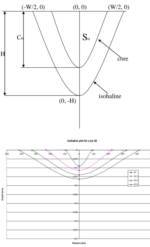
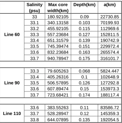
Figure 4 shows the CalCOFI station locations and the vertical sections of mean salinity for July along CalCOFI stations 60, 90 and 110. The low-salinity pool is visible in these sections as a distinct core. We choose to model the isohalines in the low-salinity core using a series of

parabolas having their foci on the same vertical (see Figure 5a). This vertical line passes through the center of the core, is the axis of all the parabolic isohalines and is perpendicular to the

directrix of the set of parabolas.

The parabolic formulation for the low salinity pool for a point (x, z) (Fig. 5a) is given by:

) ( 4 2 H z a x   (1)

where H is the depth of the isohaline core, and the parabolic isohaline has vertex at (0, -H) in the X-Z plane (Fig. 5a).

At the surface, where z = 0, we can use the salinity data obtained by Lynn et al. (1982) and presented by (Lynn and Simpson, 1987) for evaluating the ―a‖ values of the parabolic isohalines.

Specifically, for the surface points of each parabolic isohaline, one can write a simple

relationship between the maximum width (W) of the pool and the depth (H) of the isohaline as: (W/2)2 = 4aH; which leads to a = (1/H)(W/4)2. Using the observed width and depth of each of the isohalines for each of the sections in Figure 4, the ―a‖ values of these parabolas were obtained. These data have been tabulated in Table 3. The modeled parabolic isohalines corresponding to Line 60 are shown in Figure 5b, and they compare reasonably well with the observed isohalines shown in Figure 4b.

We next distinguish between the ―core‖ area of the pool and the parabolic isohalines outside the core. The salinity in the core area is assumed to be constant, S0, from surface to the

core depth (C0) bounded by the parabolic isohaline of S0 in the x-z vertical section. Thus, from a

feature model perspective, given a specific set of S0, C0, we now need to find the salinity at each

As we have seen above, the parabolic assumption allows one to compute the ―a‖ value for different ―H‖ and once these are plotted, it was noted that, for increasing value of H, ―a‖ increases almost linearly, which led us to relate ‗H‘ and ‗a‘ by the following equation

0 ) (a C a H H           (2)

where C0 is the core depth.

Plugging the value of H in equation 1 we have

                 _{1 0} 2 1 4 (a) C a H z a x .

Rearranging terms, a quadratic in ―a‖ can be formed

0 4 ) )( ( ) ( 2 1 0 1 2 _                  x a C z a a H

whose real solution is given by:

                            a H x a H C z C z a 2 ) ( ) ( ) ( 2 / 1 2 1 2 0 1 0 1 (3)

Thus, once we get an ‗a‘, we can use equation 2 to find out the depth, H, of the isohaline. In this way the isohaline gets defined. Analysis of the observed core (from Figure 4) at several lines

yielded an almost constant value of         a S

. Thus, similar to H of an isohaline, point-wise salinity

can now be obtained using the equation

0 ) (a S a S S           (4)

where S0 is the salinity of the core of the pool. So, it turns out that we can express S as a

function of S0, C0, and . Given these four parameters, we can now determine the

salinity (using Table 3, Equations 3 and 4) at any point in the low-salinity pool.

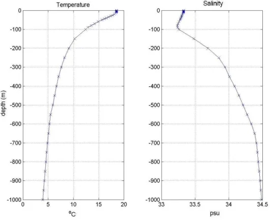
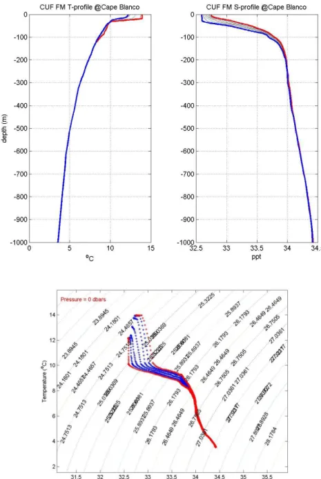
Figure 6a-b shows the temperature and salinity profiles for this core, which were adapted from Lynn and Simpson‘s (1987) analysis of the data obtained through the long-term monitoring program CalCOFI . From such a typical salinity profile, one can extract the parameters S0 and C0

for the feature model. The salinity and depth variation with ―a‖ are given by the numbers in Table 3. For the implemented feature model, the initial path of the CC is a representative one, and would have to be obtained on the basis of SST or color signatures. It is suggested that the core of the CC is better identified from color images (such as those from MODIS) as the chlorophyll boundary. In the future, when Sea surface salinity fields will be available from NASA‘s Aquarius mission, one would expect to identify this core of the CCS.

4.2 Feature Models for the California Undercurrent (CUC)

The scarcity of data for the CUC was highlighted in the overview section. The only complete and continuous profiling was done by Pierce et al. (2000), which is shown in Figure 7. It is, however, worthwhile to note that the location of the CUC offshore of the Monterey Bay region (the focus of AOSN-II during summer 2003) was highly variable. Early observations of the CUC in this region (36N to 37N) by Wickham (1975) indicated a complex alongshore flow near the coast, in both poleward and equatorward directions in the upper 500 m offshore close to 123W. In particular, he observed a poleward flow being subdivided into two parts by a strong (60 cm/sec) equatorward jet down to 500 meters (Fig. 11 of Wickham, 1975). The recent NMFS

a S   a H  

at 36.47N and at 36.8N, while flowing very close to the coast north of 37N (see Fig. 4b of Pierce

et al., 2000). A section at 35.97N shows a clear equatorward jet in the middle of the weak

poleward flow.

In fact, Rischmiller (1993) found that the area of poleward flow off of Point Sur extended well beyond the upper continental slope up to a distance of 200 km from the coast and to a depth of 750-1000 m or greater (Garfield et al., 1999). Based on Lagrangian drifters during 1992-95, Garfield et al. (1999) plotted the ensemble and individual spaghetti diagrams (Figs. 5 and 6 of their paper), which clearly show that the CUC flow is further offshore across the Monterey Bay region than it is to the north of this region.

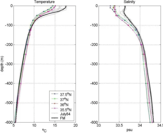
With this background, we have identified the July 1984 CalCOFI data set (analyzed by Pierce et al. 2000) as a candidate analysis data set for the basis of a CUC template. A first-order feature model for the CUC will be implemented on the basis of this data set from July 1984, and other supporting temperature-salinity observations. These feature model profiles are shown in Figure 8. Preliminary analysis suggests that a warm and saline water mass can be traced at 200-300 m depth. Curiously, the path of this water mass follows the 2500 m isobath in the latitudinal range of 34-37.5N. This offshore trajectory resembles the single drifter trajectory of Garfield et

al. (1999), as was shown in their Figure 6.

At depth, the CUC is observed to shed eddies. Garfield et al. (1999, 2001) tracked 38 approximately isobaric RAFOS floats ballasted at 300m in the CUC. They found 2 size-classes of eddies: small (radius < 35 km) rapidly anticyclonically rotating submesoscale coherent vortices (that they called ―cuddies‖), and larger (radius >50 km) eddies formed due to other processes such as baroclinic instability. They found that the cuddies propagate westward into the

interior with speeds of 1-2 cm/s (see their Figure 5). We will show later that the feature-modeled CUC develop eddies similar to these at subsurface depths during the dynamical simulations.

4.3 Coastal Upwelling Front Feature Model

This subsection documents the feature models of the coastal upwelling fronts. Six locations are chosen for the upwelling sites – Cape Blanco, Cape Mendocino, Pt. Arena, Pt. Reyes, Pt. Año Nuevo and Pt. Sur. For the estimate of the upwelling front feature model, two temperature profiles are required: one for inshore and the other for offshore. Base data were obtained from various sources and various cruises listed in Table 1 of Kim et al. (2007).

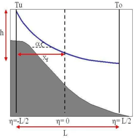
The upwelling feature models for each cape follow the methodology of Shaji and Gangopadhyay (2007). An upwelling feature model requires the specification of two T and S profiles – an inshore profile and an offshore profile, which are dynamically interpolated with a

tanh function (see Shaji and Gangopadhyay (2007) and Calado et al. (2008) for details).

The upwelling region‘s temperature is given by,

T(η; z) = To(z) + [Tu(z) - To(z)] m(η, z) (5)

where

m(η, z) = ½ + ½ tanh [(η – θz )/λ]

is a melding function, η is the cross-frontal distance from the axis of the front, and z is positive vertically upward. T(η, z) is the upwelling regional temperature distribution, Tu(z) is the

upwelling nearshore temperature profile, and To(z) is the offshore temperature profile. θz is the

slope of the front, and λ is the e-folding half-width of the front (= L/2) (see Figure 9).

offshore T and S (red) and derived FM T/S profiles (blue) are compared to show the range captured by the feature model.The resulting upwelling section at initialization is shown in Figure 11. Clearly such initialization would have significant impact on the predictive capability of a forecast system in the shallow coastal region of the CCS. Similar constructs of the upwelling FMs were derived and implemented for the other five Capes.

5. Synoptic Initialization, Model Domain and Numerical Parameters

As indicated in Section 1, feature-oriented methodology requires the development of a synoptic circulation template for the region. This template is designed from a feature-based synthesis of the regional circulation pattern. From it, a map of strategic sampling locations for placing feature model profiles is produced; it provides ''synthetic synoptic expressions'' for fronts, eddies, gyres, and other circulation structures and water masses at the initialization or model-updating phase. A suitable climatology is then selected to provide the background of the synoptic features. Further, a multiscale objective analysis (OA; Lermusiaux, 1999a,b) is

performed to meld the synoptic and large-scale fields, which results in a three-dimensional field for initializing a numerical model grid. In this section, we describe the initialization procedure, followed by the details of the selected model domain and its parameters.

5.1. Construction of Synoptic Initialization Using the Feature-based Multi-scale

Synthesis

Figure 12 shows an example of the synoptic circulation template for the CCS region. The major advantage in using such a template is the ability to resolve synoptic structures on the basis of past oceanographic knowledge of the region, even when there is a lack of observations for the synoptic features. The red, black and blue stars in Figure 12 represent the high-resolution

sampled stations where the feature model (FM) temperature and salinity profiles are provided to resolve three individual synoptic features. In this region, the CCS (red stars), the CUC (black stars) and the upwelling regions (blue stars) are the primary synoptic features that are represented in the circulation template. The axis of the core of the CC is determined as a line parallel to a smoother version of the coastline at about 500km offshore. The locations of the perimeter of the upwelling regions are all based on historical observations around the capes. Note that only a limited number (~100) of stations are needed to describe the synoptic behavior of this region. These are again placed based on a handful of FM parameters described in Section 4.

Once the feature models are developed (as described in Section 4), an initialization field is then generated by objectively analyzing the synthetic FMs on the synoptic template in a selected background climatology for a multi-scale synthesis. The green stars in the circulation template in Figure 12 are the locations of the Boyer et al. (2005) ¼ -degree climatology data. The multiscale OA is, in fact, done in two stages. In the first stage, the largest dynamical scales are resolved at each level, using estimated large-scale e-folding spatial decays, zero-crossings and temporal decay. The background for the first stage OA is the horizontal average of the climatological data. In the second stage of the OA, the synoptic mesoscale phenomena are resolved using their estimated space-time scales. The background for this OA is the first stage OA. Once the initialization field is available as a result of the multi-scale synthesis, any numerical model can then be used for nowcasting, forecasting and dynamical process studies with such initialization fields.

We use Boyer et al.‘s (2005) temperature and salinity fields objectively analyzed for August with ¼ degree of spatial resolution. The method of objectively analyzing the data is the

technique necessitated by the different scales of the analysis. In the one-degree analysis, the radius of influence is 250 km; in the quarter-degree analysis, the radius of influence is 40 km.

5.2. The POM Parameters and Domain Setup

Initialization of any dynamical model requires the specification of each prognostic variable at each grid point of the three-dimensional model domain. In this work we chose the terrain-following coordinate system for this implementation of the Princeton Ocean Model – POM (Ezer and Mellor, 1994; Blumberg and Mellor, 1987 and Ezer and Mellor, 1997). The domain consists of 150 x150 grid points in the horizontal with 8 km resolution and 31 vertical levels. The model is limited geographically by 34.38N, 48.82N and -138.22E, -118.68E.

The model bathymetry is based on the ETOPO5 data set. The depth range is 5 to 6000 m. On the north, south and west we used open boundary conditions. Along these boundaries the model's thermohaline structure was held to initial temperature and salinity values via partially-clamped boundary conditions (Blumberg and Kantha, 1985). Also, a radiation condition based on Summerfield's equation was applied to the baroclinic velocities on the open boundaries. Flather radiation condition (Palma and Matano, 1998) was applied to the barotropic velocities, and a non-gradient condition for the free sea surface elevation was employed as well.

As a consequence of the relaxation in the temperature-salinity fields, we imposed a geostrophic flow at the model's open boundaries through the inclination of the isopycnal

surfaces. In other words, the climatological signal, rendered by the inclinations of the isothermal and isohaline surfaces, contains the signal of both the velocity component generated by wind forcing and the component associated with the thermohaline circulation. The wind forcing was generated from the mean August field extracted from QuikScat data (Graf et al., 1988). We also

included the deep CUC, underlying the CC, in the regional modeling, as well as the influence of the thermohaline circulation component on the mesoscale activity in the region of interest.

5.3 Initialization Strategy for Short-term Forecasting with POM

Synoptic short-term simulations require three-dimensional specifications of initial fields of T, S, u and v. However, the standard practice for basin-scale numerical modeling exercises is to specify T and S only, with zero velocity (Ezer and Mellor, 1994; Ezer and Mellor, 1997; Mathew and McClean, 2005). The basin-scale approach requires models to develop the inertia fields in a one-to-ten years long "spin-up'' period. As mentioned earlier, our goal is to develop a system for short-term synoptic forecasting where we cannot afford to run models over a long spin-up period. Thus, specifying the best possible velocity field in addition to the mass (T and S) field becomes mandatory for synoptic short-term simulations. Adjustments to wind forcing and baroclinic internal adjustment are also necessary for synoptic forecasting.

Previous work on such adjustment procedures included the Harvard Ocean Prediction System (HOPS) in the studies of Gangopadhyay et al. (1997, 2003) and Brown et al. (2007 a, b), the Regional Ocean Modeling System (ROMS) by Shaji and Gangopadhyay (2007) and Kim et

al. (2007), and a first application with POM by Calado et al. (2008). The strategy for setting up

POM in the CCS region was carried out using climatological temperature and salinity initial fields following Ezer and Mellor‘s (1997) methodology, with the additional implementation of geostrophic velocity as initial condition for the baroclinic velocities, balanced with initial T-S field. Specifically, we held the T and S fields fixed over the first five days of simulation in the diagnostic mode, an approach described by Ezer and Mellor (1997). These authors used this

underlying mass field and to the topography. A similar technique for initializing POM with geostrophic velocities was used by Castelao et al. (2004) to study shelf break upwelling in the region of southeastern Brazil. The initial geostrophic velocity was computed from the

temperature and salinity by the OA methodology described by Lozano et al. (1996). A

representative initial field of temperature, salinity and velocity can be seen for day 1 in Figure 13 (left-top) and Figure 14 (left-top).

6. Dynamical Simulations with Feature Models

The long-term goal of this study is to develop the capability of nowcasting and forecasting using the FORMS technique in the CCS region. So far, we have discussed the development of a set of appropriate feature models for this region and their incorporation into a multiscale objectively analyzed initialization. In this section we describe the results of a 40-day simulation with such initialization using the POM setup described above.

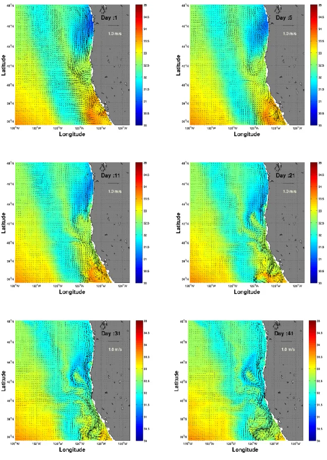
6.1 The Surface Temperature and Salinity Evolution

Figures 13 and 14 show the evolution of the CCS-FORMS initialization for a typical summer synoptic realization. Temperature fields (with current vectors superposed) for days 1, 5, 11, 21, 31 and 41 are shown in the six panels in Fig. 13 as marked. The initial field shows the upwelling around the capes and the southward-flowing current with the low-salinity pool (Figure 14a) identified as the CC core. A continuous southward-flowing current develops along the coast by day 11. Additionally, a narrow region similar to the coastal transition zone develops during the third week.

at 42N and at 38N. Based on CTZ satellite and field data analyses during May-July 1987 and 1988, Strub et al. (1991) determined the existence of a surface meandering jet surrounded by a field of eddies between 36 and 42N. Large dynamic height ranges corresponding to more well-developed eddies were found. The authors maintained that the eddies occurred mostly inshore of the jet north of 39N, and were both inshore and offshore of the jet south of 39N. In our simulations, starting with the jet and upwelling regions in the FORMS setting, a large eddy inshore of the jet is formed around 42N. A number of additional eddies (both cyclonic and anti-cyclonic) were also generated during the simulation (Fig. 13d, e, f). On the larger scale, it is interesting to note that the dynamical evolution of the temperature field is similar to the synoptic SST shown in Figure 1a, indicating the robustness of the model simulations.

The salinity evolution is shown in Figure 14. Note how the low-salinity core of the CCS is initialized as a jet feature model and how it dynamically adjusts and evolves during the simulation while interacting with the surrounding waters. The high salinity signature of the eddy development at 42N is clearly seen within the spread of the low-salinity coastal waters. The boundary of the coastal transition zone is probably best designated by the dynamic narrow band of high-salinity between the low-salinity core of the CC and upwelling regions along the coast. The mesoscale eddy evolution during the first month of simulation at the surface is presented in Figure 15 (a-f) in terms of eddy kinetic energy. Figure 16 shows the evolution of this mesoscale field in a near coastal focused region.

Several realistic features are observed during the 5-30 days of simulation as presented in Figure 16. First, an anticyclone off Monterey Bay is seen by day 5 at 37N. This is accompanied by a small paired cyclone at 38N. The cyclone continues to grow and maintain itself through day

part anticyclone-cyclone-anticyclone system by day 20, which persists through day 30. In the northern part of the domain, a cyclone at 42-43N, 126-127W is apparent by day 10, which moves NW continuously through day 30. This eddy is originally connected with the upwelling at Cape Mendocino (41.5N). A quick succession of cyclones and anticyclones are observed near 40N. This region near 40N, 126W can be identified as the most variable region in the simulation.

Specifically, the series of cyclones and anticyclones developed by day 20 (Figure 16, left-bottom) warrants further discussion. This evolution resembles the schematic in Figure 2: the middle as well as the 3rd panel indicates that the dynamical evolution of the CCS is a combination of the series of eddies and the jet-meander-eddy system. The simulated convergent shelf flow near Cape Mendocino was observed and described by Magnell et al. (2003). An anticyclonic eddy similar (albeit smaller) to the observed seasonally recurring giant eddy recently described by Crawford et al (2009) is simulated near 39N, 125W.

Next section describes the evolution of the undercurrent and its associated eddies which are shown in Figures 17 through 19. Figure 20 shows a Chlorophyll image (for September 2004) along with the model evolution on day 20. Interestingly, there are distinct resemblances in the eddy activity in a number of sub-regions between the independent image and the simulated temperature field which was evolved by POM starting from the feature-based initialization without any eddy field (See Figure caption for details). Such comparisons will be quantified in a hindcast mode in future for multiple hindcasts to help develop an operational forecasting system for the CCS.

6.2 Subsurface Evolution (300 m and 1000 m)

temperature salinity and velocity fields at 300 m. The subsurface eddies are visible in both temperature and salinity fields. Since the low-salinity pool of the CC core was feature-modeled to be restricted vertically above 160 m, it does not penetrate to the intermediate depths. The subsurface signature of the surface eddies at 42N and 38N is visible in Figs. 17a-b. Figure 18 shows the mesoscale evolution near the coast inshore of 130W during the first four weeks of the simulation. The subsurface signature of the surface eddies at 36N (the ACE-CE-ACE triad) is evident on day 20. By day 30 this evolves into a CE-ACE pair similar to that at the surface.

The 1000 m flow evolution is presented in Figure 19 for days 1, 5, 10, 20, 30 and 40. It is clear from the simulation that, in addition to forming subsurface eddies, there is a natural

tendency of poleward flow development along the California coast. Note that this coastal undercurrent is the natural pathway for the low-oxygen, nutrient-rich water, which originates in the eastern tropical Pacific. Thus, the FORMS-CCS could be useful for predicting the

biogeochemistry of the California Current System in the future.

A series of anticyclonic eddies developed near the coast inshore of the poleward flow during the simulation. By day 5, an ACE develops first near the coast at 37N. A poleward continuous flow develops at 1000m by day 10. The ACE at 37N grows between day 10 and day 40. By day 20, a second ACE is formed inshore of poleward flow at around 40-41N, which grows in size by day 30. A third inshore ACE is seen to develop at 44N around day 40. In addition to the ACEs, an ACE-CE pair was observed between 36 and 38N (similar to the surface pair) on day 20. The smaller CE signature dissipated by day 30. Table 4 summarizes the sizes and nature of the simulated eddies discussed above along with some observational evidence of these eddies in past studies.

7. Conclusion

This study described the development of a first-order feature-oriented regional modeling system (FORMS) for the California Current system. The synoptic circulation features include the mean flow and southeastward meandering jet(s) of the California Current, the poleward California Undercurrent and six upwelling regions along the western coast of the U.S. (Figure 3). We identified the typical synoptic width, location, vertical extent, and core characteristics of these features and their dominant spatial and temporal scales of variability from past observational, theoretical and modeling studies, which are listed in Table 1. These synoptic features were then melded with available climatology of the region for initialization.

Dynamical simulations over a 40-day period using POM illustrate the applicability of FORMS to a transient eastern boundary current region such as the CCS. The simulations initialized with FORMS realistically evolved various interactions among the low salinity pool, the background climatology and the upwelling regions. A number of anticyclones and cyclones appeared at places where observational evidences of such eddies were documented in previous studies. These are listed in Table 4. In addition, a countercurrent develops in the intermediate to deep waters along the coast, which sheds realistic eddies (―cuddies‖) near a number of capes.

This physical phenomenological validation is the first step towards building a FORMS-based prediction system for this region. The next step would be to statistically validate such simulations (initialized with low-salinity pool, coastal upwelling, CUC, CC, eddies and background climatology) following the works of Robinson and Gangopadhyay (1997) for the western North Atlantic. Calibration of such a system for MB03 and MB06 and other hindcast studies will lead to a robust implementation of an operational system for the CCS in the near future.

Acknowledgement

This work was funded by the Office of Naval Research grants 03-1-0411 and N00014-03-1-0206 at the University of Massachusetts at Dartmouth. Leslie Rosenfeld‘s participation was supported by ONR grant N00014-03-WR-20009. Our special thanks to Dr. Jim Bellingham and his group at MBARI for numerous informative discussions and making the data available from the MUSE and AOSN2 experiments. We are grateful to all who contributed to this effort by providing datasets. We would, especially like to acknowledge Drs. Ken Brink, Tommy Dickey, Francisco Chavez, Toby Garfield, Alex Warn-Varnas, Shaun Johnston, Curt Collins, Margaret McManus, Libe Washburn, and Erika McPhee-Shaw for their help and support in procuring the datasets from various sources. We appreciate the editorial assistance provided by Mr. Frank Smith and graphics help of Ms Carolina Nobre at SMAST. This is our final AOSN Contribution.

References

Abbott, M.R., and P.M. Zion, 1987. Spatial and temporal variability of phytoplankton pigment off Northern California during CODE-1. J. Geophy. Res. 92, 1745-1756. Abbott, M.R., and B. Barksdale, 1991. Phytoplankton Pigment Patterns and Wind Forcing

off Central California. J. Geophys. Res., 96, 14,649-14,667.

Allen, J. S., L.J. Walstad, and P.A. Newberger, 1991. Dynamics of the Coastal Transition Zone Jet, 2. Nonlinear finite amplitude behavior, J. Geophys. Res., 96, 14,995-15,016.

Barth, J.A. and D.M. Checkley, 2009. Patterns and processes in the California Current System, Progress in Oceanography, 83, 49-64.

Barth, J.A., S.D. Pierce and R.L. Smith, 2000. A separating coastal upwelling jet at Cape Blanco, Oregon and its connection to the California Current System. Deep Sea

Research II, 47, 783 – 810.

Belkin, I.M., P.C. Cornillon and K.Sherman, 2009. Fronts in Large Marine Ecosystems. Progress In Oceanography, 81(1-4), 223-236.

Bennett, A. F., 1992. Inverse Methods in Physical Oceanography. Cambridge Un. Press, Cambridge, 346 pp.

Bennett, A. F., 2002. Inverse Modeling of the Ocean and Atmosphere. Cambridge Un. Press, Cambridge, 234 pp.

Bernstein, R.L., L. Breaker, and R. Whitner, 1977. California Current eddy formation: Ship, air and satellite results. Science, 195, 353-359.

Blumberg, A.F. and L.H. Kantha, 1985. Open boundary condition for circulation models. J.

Hydarul. Eng. – ASCE 111 (2), 237–255.

Blumberg, A.F. and G.L. Mellor, 1987. A Description of a Three Dimensional Coastal Ocean Circulation Model. In: N.S. Heaps, Editor,Three-dimensional coastal ocean models, American Geophysical Union, Washington (1987),1–16.

Boyer, T., S. Levitus, H. Garcia, R.A. Locarnini, C. Stephens and J. Antonov, 2005. Objective analyses of annual, seasonal, and monthly temperature and salinity for the World Ocean on a 0.25° grid. International Journal of Climatology, 25(7), 931–945.

Brown, W. S., A. Gangopadhyay, F. L. Bub, Z. Yu and G. Strout, and A. R. Robinson, 2007a. An Operational Circulation Modeling System for the Gulf of Maine/Georges Bank Region, Part 1: The Basic Elements. IEEE J. Oceanic

Engineering, 32 (4), 807-822.

Brown, W. S., A. Gangopadhyay, and Z. Yu, 2007b. An Operational Circulation Modeling System for the Gulf of Maine/Georges Bank Region, Part 2: Applications. IEEE

J. Oceanic Engineering, 32 (4), 807-822.

Brink, K.H., R.C. Beardsley, P.P. Niiler, M. Abbott, A. Huyer, S. Ramp, T. Stanton, and D. Stuart, 1991. Statistical properties of near-surface flow in the California coastal transition zone. J. Geophys. Res., 96, 14,693-14,706.

Brink, K.H. and T.J. Cowles, 1991. The coastal transition zone program. J. Geophys. Res.,

96, 14,637-14,647.

Brink, K. H., R. C. Beardsley, J. Paduan, R. Limeburner, M. Caruso, and J. G. Sires, 2000. A view of the 1993-1994 California Current based on surface drifters, floats, and remotely sensed data. Journal of Geophysical Research, 105(C4), 8575-8604. Bucklin, A., 1991. Population Genetic Responses of the Planktonic Copepod Metridia

pacifica to a Coastal Eddy in the California Current, J. Geophys. Res., 96,

14,799-14,808.

Calado, L, A. Gangopadhyay and I.C. daSilveira, 2008: Feature-Oriented Regional Modeling and Simulations (FORMS) For the Western South Atlantic, Southeastern Brazil Region. Ocean Modeling (25), 48-64.

Calado, L., A. Gangopadhyay, and I. C. A. da Silveira, 2006. A parametric model for the Brazil Current meanders and eddies off southeastern Brazil, Geophys. Res. Lett.,

33, L12602, doi:10.1029/2006GL026092.

Capet, X., J. C. McWilliams, M. J. Molemaker, A. F. Shchepetkin, 2008: Mesoscale to Submesoscale Transition in the California Current System. Part I: Flow Structure, Eddy Flux, and Observational Tests. J. Phys. Oceanogr., 38, 29–43.

Capet, X., J. C. McWilliams, M. J. Molemaker, A. F. Shchepetkin, 2008: Mesoscale to Submesoscale Transition in the California Current System. Part II: Frontal Processes. J. Phys. Oceanogr., 38, 44–64.

Castelao, R.M., E.J.D. Campos and J.L. Miller, 2004. A Modelling Study of Coastal Upwelling Driven by Wind and Meanders of the Brazil Current. Journal of

Coastal Research, (July 2004), 662 – 671.

Chao, Y., Z. Li, J. Farrara, J. C. McWilliams, J. Bellingham, X. Capet, F. Chavez, J.-K. Choi, R. Davis, J. Doyle, D. Fratantoni, P. Li, P. Marchesiello, M. A. Moline, J. Paduan, and S. Ramp, 2008. Development, implementation, and evaluation of a data-assimilative ocean forecasting system off the central California coast. Deep-Sea

Research II, doi:10.1016/j.dsr2.2008.08.011.

Chavez, F.P. and C. Collins,eds, 2000. Studies of the California Current System Part 2,

Deep-Sea Research II, 47, 5-6.

Chavez, F.P. and C.A. Collins, 2000. Studies of the California Current System: present, past and future. Deep-Sea Research II, 47, 761-763.

Chelton, D. B., 1984. Seasonal variability of alongshore geostrophic velocity off central California. J. Geophys. Res., 89, 3473–3486.

Chavez, F. P., T.J. Pennington, R. Herlien, H.W. Jannasch, G. Thurmond and G. Friederich, 1997. Moorings and drifters for real-time interdisciplinary oceanography, J.

Atmos. and Ocean. Tech., 14, 1199-1211.

Chavez, F.P., R.T. Barber, P.M. Kosro, A. Huyer, S.R. Ramp, T.P. Stanton, and B. Rojas de Mendiola, 1991. Horizontal transport and the distribution of nutrients in the

Chelton, D. and M. Schlax, 1991. Estimation of time averages from irregularly spaced observations: With application to Coastal Zone Color Scanner estimates of chlorophyll concentration. J. Geophys. Res., 96, 14,669-14,692.

Chereskin, T.K. and P.P. Niiler, 1994. Circulation in the Ensenada Front—September 1988.

Deep Sea Research Part I: Oceanographic Research Papers, 41, 1251-1287.

Collins, C.A., J.T. Pennington, C.G. Castro, T.A. Rago and F.P. Chavez, 2003. The California Current system off Monterey, California: physical and biological coupling. Deep-Sea Research 11 50 (2003) 2389-2404

Collins, C.A., C.G. Castro, H. Asanuma, T.A. Rago, H.-K. Han, R. Durazo, and F.P. Chavez, 2002. Changes in the hydrography of Central California waters associated with the 1997-98 El Niño. Progr. in Oceanog., 54, 184-204.

Collins, C.A., N. Garfield, T.A. Rago, F.W. Rischmiller, and E. Carter, 2000. Mean Structure of the Inshore Countercurrent and California Undercurrent off Point Sur,

California. Deep Sea Res., 47, 765-782.

Collins, C. A., N. Garfield, R.G. Paquette, and E. Carter, 1996. Lagrangian Measurement of subsurface poleward Flow between 380N and 430N along the West Coast of the United States during Summer, 1993. Geophys. Res. Letters, September 1, 1996,

23, No. 18, 2461-2464.

Cornuelle, B.D., T.K. Chereskin, P.P. Niiler, M.Y. Morris, and D.L. Musgrave, 2000. Observations and Modeling of a CA, Undercurrent Eddy,‖ J. Geophys. Res., C 105, 1227-1243.

Crawford G. and S. Stone, 2008. COCMP Surface Current Mapping Reveals. Eddy and Upwelling Jet off Cape Mendocino. American Geophysical Union, Fall Meeting 2008, abstract #OS41B-1216.

Cummings, J.A., C. Szczechowski and M. Carnes, 1997. Global and regional ocean thermal analysis systems. Marine Tech. Soc. J., 31, 63-75.

Dewey, R.K., J.N. Moum, C.A. Paulson, D.R. Caldwell, and S.D. Pierce, 1991. Structure and dynamics of a coastal filament, J. Geophys. Res., 96, 14,885-14,907.

Ezer, T and G.L. Mellor, 1994. Diagnostic ands prognostic calculations of the North Atlantic circulation and sea level using a sigma coordinate ocean model. J. Geophy. Res.,

99, 14,159 – 14,171.

Ezer T. and G.L. Mellor, 1997. Data assimilation experiments in the Gulf Stream region: how useful are satellite-derived surface data for nowcasting the subsurface fields? J Atmos Ocean Tech, 16(6), 1379–1391.

Flament, P., L. Armi, and L. Washburn, 1985. The evolving structure of an upwelling filament. J. Geophys. Res., 90:1765-1985.

Fox D.N., M.R. Carnes and J.L. Mitchell, 1992. Characterizing Major Frontal Systems: A Nowcast /Forecast System for Northwest Atlantic. Oceanography, 5, 49-53. Fratantoni, D.M. and S. H. D. Haddock, 2009. Introduction to the Autonomous Ocean