From light edges to strong edge-colouring of 1-planar graphs

HAL Id: hal-02112188

https://hal.archives-ouvertes.fr/hal-02112188v3

Submitted on 17 Dec 2019

HAL is a multi-disciplinary open access

archive for the deposit and dissemination of

sci-entific research documents, whether they are

pub-lished or not. The documents may come from

teaching and research institutions in France or

abroad, or from public or private research centers.

L’archive ouverte pluridisciplinaire HAL, est

destinée au dépôt et à la diffusion de documents

scientifiques de niveau recherche, publiés ou non,

émanant des établissements d’enseignement et de

recherche français ou étrangers, des laboratoires

publics ou privés.

From light edges to strong edge-colouring of 1-planar

graphs

Julien Bensmail, François Dross, Hervé Hocquard, Eric Sopena

To cite this version:

Julien Bensmail, François Dross, Hervé Hocquard, Eric Sopena. From light edges to strong

edge-colouring of 1-planar graphs. Discrete Mathematics and Theoretical Computer Science, DMTCS,

2020, vol. 22 no. 1 (2). �hal-02112188v3�

From light edges to strong edge-colouring of

1-planar graphs

Julien Bensmail

François Dross

Hervé Hocquard

Éric Sopena

1

Université Côte d’Azur, CNRS, Inria, I3S, France

2

Univ. Bordeaux, CNRS, Bordeaux INP, LaBRI, UMR 5800, F-33400, Talence, France

received 26th_{Apr. 2019, revised 29}th_{Nov. 2019, accepted 29}th_{Nov. 2019.}

A strong edge-colouring of an undirected graph G is an edge-colouring where every two edges at distance at most 2 receive distinct colours. The strong chromatic index of G is the least number of colours in a strong edge-colouring of G. A conjecture of Erd˝os and Nešetˇril, stated back in the 80’s, asserts that every graph with maximum degree ∆ should have strong chromatic index at most roughly 1.25∆2. Several works in the last decades have confirmed this conjecture for various graph classes. In particular, lots of attention have been dedicated to planar graphs, for which the strong chromatic index decreases to roughly 4∆, and even to smaller values under additional structural requirements. In this work, we initiate the study of the strong chromatic index of 1-planar graphs, which are those graphs that can be drawn on the plane in such a way that every edge is crossed at most once. We provide constructions of 1-planar graphs with maximum degree ∆ and strong chromatic index roughly 6∆. As an upper bound, we prove that the strong chromatic index of a 1-planar graph with maximum degree ∆ is at most roughly 24∆ (thus linear in ∆). The proof of this result is based on the existence of light edges in 1-planar graphs with minimum degree at least 3.

Keywords: strong edge-colouring, strong chromatic index, 1-planar graphs, light edges.

1

Introduction

Planar graphsare those graphs which can be drawn in the plane in such a way that no two edges cross. Colouring planar graphs has been one of the most active fields of graph theory, due in particular to the investigations that led to the well-known Four-Colour Theorem [1, 2]. Since then, whenever considering new graph problems, it generally makes sense wondering what happens for planar graphs. These graphs, however, are far from catching the structure of real-world graphs; for a given problem, one possible next direction can thus be to consider graph families that enclose planar ones.

One of the most natural generalizations of planar graphs is that of 1-planar graphs, which are those graphs that can be drawn on the plane in such a way that every edge is crossed at most once. These graphs were first considered by Ringel [22], as he was investigating a possible generalization of the Four-Colour Theorem. Since then, many aspects of 1-planar graphs have been considered in the literature, including structural aspects, colouring aspects, topological aspects, and so on. We refer the interested reader to the recent survey by Kobourov, Liotta and Montecchiani on this topic [18].

Our goal in this work is to initiate the study of the strong chromatic index of 1-planar graphs. For a graph G, a strong edge-colouring of G is an edge-colouring where no two edges at distance at most 2 are assigned the same colour. To make it more precise, let us recall that two edges e, f are at distance 1 if they share an end, while e and f are at distance 2 if they are not at distance 1 and an end of e is adjacent to an end of f . A strong edge-colouring of G can thus also be regarded as an edge-partition of G into induced matchings, or as a proper vertex-colouring of the square of the line graph of G. The strong chromatic index of G, denoted χ0_s(G), is the least number of distinct colours assigned by a strong edge-colouring of G.

The notion of strong edge-colouring was first introduced by Fouquet and Jolivet [12]. One of the leading conjectures in this field is that of Erd˝os and Nešetˇril [9], stated back in the 1980’s (when no confusion is possible, we here and further denote by ∆ the maximum degree of a given graph):

2 J. Bensmail, F. Dross, H. Hocquard, É. Sopena

Conjecture 1.1 (Erd˝os, Nešetˇril [9]). For every graph G, we have χ0_s(G) ≤ (₅ 4∆ 2 _{if ∆ is even,} 1 4(5∆ 2_{− 2∆ + 1) if ∆ is odd.}

Conjecture 1.1 is still wide open in general. It was verified for graphs with maximum degree ∆ = 3 by Andersen [3] and Horák, Qing and Trotter [16], while, already for every ∆ ≥ 4, it is not known whether the conjecture is true or not. To date, certainly the most investigated class of graphs is that of planar graphs, which were first considered by Faudree, Gyárfás, Schelp and Tuza [11]. Using a nice combination (to be described in Section 3) of the Four-Colour Theorem and Vizing’s Theorem, they proved that every planar graph G has strong chromatic index at most 4∆ + 4, while, for every ∆ ≥ 2, there exist planar graphs with maximum degree ∆ and strong chromatic index 4∆ − 4. Thus, roughly speaking, the maximum value of the strong chromatic index of a planar graph with maximum degree ∆ is of order 4∆.

Theorem 1.2 (Faudree et al. [11]). For every ∆ ≥ 2, the maximum strong chromatic index over all planar graphs with maximum degree∆ lies in between 4∆ − 4 and 4∆ + 4.

Many works aimed at investigating conditions for the strong chromatic index of planar graphs to drop to roughly 3∆ and even 2∆. Such conditions notably involve the value of ∆, of the girth (i.e., length of a smallest cycle), and of the maximum average degree (i.e., density of a densest subgraph). See [5, 7, 13, 15, 19] for several works in that line.

In this work, we give first results towards understanding how the strong chromatic index of 1-planar graphs behaves. In Section 3, we establish that the maximum value of the strong chromatic index over all planar graphs is of order at most roughly 24∆ (Corollary 3.4), while, for every ∆ ≥ 5, there exist 1-planar graphs with maximum degree ∆ and strong chromatic index roughly 6∆ (Proposition 3.1). Although our upper bound is probably far from tight, it indicates that 1-planar graphs is yet another class of graphs for which the maximum strong chromatic index is linear in ∆, and not quadratic in ∆ as stated in the Erd˝os-Nešetˇril bound from Conjecture 1.1.

The proof of our upper bound makes use of the presence, under some circumstances, of light edges in 1-planar graphs, which are edges whose ends’ degree sum is somewhat small (i.e., bounded by a constant), in the following sense. By a k-vertex of a graph, we mean a vertex with degree k. By an (x, y)-edge of a graph, we mean an edge one of whose ends is an x-vertex and the other is a y-vertex. Light edges in 1-planar graphs were first studied by Fabrici and Madaras, who notably proved that 1-planar graphs are 7-degenerate, and 3-connected 1-planar graphs have (≤ 20, ≤ 20)-edges [10]. Later on, Hudák and Šugerek [17] proved that every 1-planar graph G with δ(G) ≥ 4 has a (4, ≤ 13)-, (5, ≤ 9)-, (6, ≤ 8)- or (7, 7)-edge. In the latter work, the authors also provided an optimal result regarding the existence of light edges in 1-planar graphs G with δ(G) ≥ 5. Some other results of this sort exist, see e.g. those in [18]. However, by the time where the results of the current work were obtained, no such result on light edges in 1-planar graphs G with δ(G) ≥ 3 was known. To fill in this gap, we originally proved that 1-planar graphs with minimum degree at least 3 have (≤ 29, ≤ 29)-edges. Independently, however, other comparable and even stronger results of this sort have appeared in the literature. We explain this situation in Section 2.

2

Light edges in 1-planar graphs with minimum degree 3

As an indication of what light edges one should expect to find in 1-planar graphs with minimum degree at least 3, let us mention the following conjecture of Hudák and Šugerek:

Conjecture 2.1 (Hudák, Šugerek [17]). Let G be a 1-planar graph of minimum degree 3. Then G contains a (3, ≤ 20)-, (4, ≤ 13)-, (5, ≤ 9)-, (6, ≤ 8)-, or (7, 7)-edge.

Towards that conjecture, a result we proved is the following:

Theorem 2.2. Every 1-planar graph G with δ(G) ≥ 3 has a (≤ 29, ≤ 29)-edge.

After a round of the review process the current paper has been through, we were notified by an anonymous referee of the existence of two papers, namely [20] by Li, Hu, Wang and Wang, and [21] by Niu and Zhang, in which are provided results that are quite comparable to, and even much better than, Theorem 2.2. Namely, in [20] the authors proved that every 1-planar graph G with δ(G) ≥ 2 has an (x, y)-edge with x + y ≤ 29 or a 2-alternating cycle (i.e., a cycle v0, . . . , v2m−1v0where v0, v2, . . . , v2m−2are 2-vertices), while in [21]

u1 u2

u3

u4

u5 u6

Figure 1: A 1-planar graph K_∆∗ with maximum degree ∆ ≥ 5 and strong chromatic index 6∆ − 12. the authors proved that every 1-planar graph G with δ(G) ≥ 3 has a (3, ≤ 23)-, (4, ≤ 11)-, (5, ≤ 9)-, (6, ≤ 8)-, or (7, 7)-edge.

Looking at the publication history of [20] and [21], it seems that our Theorem 2.2 was actually the first result of this sort to be publicly available online, in a previous version of the current paper [4]. This is the main reason why we keep using Theorem 2.2 in the current paper, instead of using the better results. We however omit its proof, which the interested reader can still find in [4].

Let us finally mention that using the better results from [20] and [21] in place of Theorem 2.2 in the proof of Theorem 3.3 (and thus of Corollary 3.4) would improve the obtained bounds, but by a constant additive term only.

3

Application to strong edge-colouring of 1-planar graphs

Using, in particular, Theorem 2.2, we study in this section strong edge-colourings of 1-planar graphs.

3.1

Lower bounds

Let ∆ ≥ 5, and let K_∆0 be the graph obtained from K6by attaching ∆ − 5 new pendant vertices to every

vertex. It can be observed that every two edges of K_∆0 are at distance at most 2 apart. Furthermore, K_∆0 is clearly 1-planar since K6is the biggest 1-planar complete graph (see e.g. [8]). Thus, for every ∆ ≥ 5 there

are 1-planar graphs with maximum degree ∆ and strong chromatic index 6∆ − 15.

Actually, 1-planar graphs with maximum degree ∆ ≥ 5 and slightly larger strong chromatic index exist, as attested by the following construction, depicted in Figure 1. Start from a K6on vertex set {u1, . . . , u6},

and replace each of the edges u1u2, u3u4 and u5u6by a complete bipartite graph K2,∆−4. Denote the

resulting graph by K_∆∗.

By construction of K_∆∗, all ui’s have degree ∆ (while the other vertices have degree 2), and K∆∗ is

1-planar, as attested by the fact that K6 is 1-planar (see Figure 1). Its strong chromatic index is deduced in

the following proposition.

Proposition 3.1. Every graph K_∆∗ has strong chromatic index6∆ − 12. Consequently, for every ∆ ≥ 5, there exist1-planar graphs with maximum degree ∆ and strong chromatic index 6∆ − 12.

Proof: Every edge of K∆∗ is incident to at least one of the ui’s, while the ui’s, with the exception of the

4 J. Bensmail, F. Dross, H. Hocquard, É. Sopena

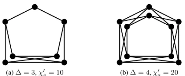
(a) ∆ = 3, χ0s= 10 (b) ∆ = 4, χ0s= 20

Figure 2: Examples of 1-planar graphs with maximum degree ∆ ∈ {3, 4} and large strong chromatic index. distance at most 2 from each other. Consequently, no two edges of K_∆∗ can receive the same colour by a strong edge-colouring, and thus χ0_s(K_∆∗) = |E(K_∆∗)| = 6∆ − 12.

For smaller values of ∆, i.e., ∆ ∈ {3, 4}, some blown-up C5’s are examples of 1-planar graphs with

larger strong chromatic index (see Figure 2). The blown-up C5with maximum degree 3 is an example of

a 1-planar graph with maximum degree 3 and strong chromatic index 10, which is the maximum possible value for the strong chromatic index of a graph with maximum degree 3 (as proved in [3, 16]). The blown-up C5with maximum degree 4 is an example of a 1-planar graph with maximum degree 4 and strong chromatic

index 20. While Erd˝os and Nešetˇril have conjectured that this is the maximum strong chromatic index of a graph with maximum degree 4 (recall Conjecture 1.1), this has not been proved yet. We however know that the strong chromatic index of a graph with maximum degree 4 is at most 21, as recently proved by Huang, Santana and Yu [14]. Thus, it might be that there exist 1-planar graphs with maximum degree 4 and strong chromatic index 21, in case the Erd˝os-Nešetˇril Conjecture turned out to be false.

3.2

Upper bounds

The upper bound on the strong chromatic index of planar graphs with maximum degree ∆ in Theorem 1.2 relies on a nice combination of Vizing’s Theorem and the Four-Colour Theorem. Let us recall that Vizing’s Theorem [23] states that every graph with maximum degree ∆ has a proper ∆- or (∆ + 1)-edge-colouring, i.e., a colouring (with ∆ or ∆ + 1 colours) of the edges where no two adjacent edges are assigned the same colour. The Four-Colour Theorem [1, 2] states that every planar graph has a proper 4-vertex-colouring, i.e., a colouring of the vertices with four colours where no two adjacent vertices are assigned the same colour.

The proof of the upper bound in Theorem 1.2 goes as follows. Let G be a planar graph. By Vizing’s Theorem, G admits a proper (∆ + 1)-edge-colouring φ. For every colour i assigned by φ, let us consider the i-graph Mi being the graph of the i-coloured edges being at distance exactly 2 in G. More precisely,

the vertices veof Miare those edges e of G with colour i by φ, and two such vertices veand vf are joined

by an edge in Miif the edges e and f are at distance exactly 2 in G. Translating a planar drawing of G to

one of Mi, it is not complicated to convince oneself that each Mi is planar. By the Four-Colour Theorem,

each Mithus admits a proper 4-vertex-colouring ψi. This yields a strong (4∆ + 4)-edge-colouring of G,

where each edge e gets colour (φ(e), ψφ(e)(ve)).

Unfortunately, mimicking the exact same proof for 1-planar graphs is not immediate. While Vizing’s Theorem can of course be applied on a 1-planar graph and there does exist a 1-planar analogue of the Four-Colour Theorem, namely the Six-Colour Theorem (stating that every 1-planar graph has a proper 6-vertex-colouring, as proved by Borodin [6]), it can however be noted that, when G is 1-planar, an i-graph Mimight not be 1-planar itself. To overcome this issue and get our upper bound, we will instead consider

proper edge-colourings avoiding certain patterns, that will ensure 1-planarity of every resulting i-graph Mi.

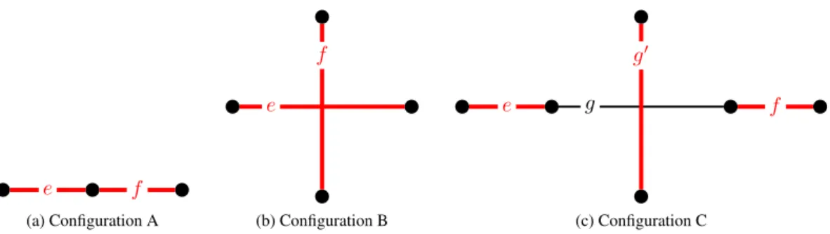
In what follows, for a 1-planar graph G, a good edge-colouring will refer to an edge-colouring φ such that none of the following three configurations appears (see Figure 3).

1. Two adjacent edges e and f receiving the same colour by φ (Configuration A). 2. Two crossing edges e and f receiving the same colour by φ (Configuration B).

3. Three edges e, f and g0receiving the same colour by φ, where e and f are at distance 2, joined by an edge g crossing g0(Configuration C).

The fact that Configuration A is forbidden implies that a good edge-colouring is always proper. It also implies that, for every colour i assigned by φ, the i-graph Mi is well defined. We now prove that the fact

e f (a) Configuration A e f (b) Configuration B e g f g0 (c) Configuration C

Figure 3: Fordibben patterns in good edge-colourings. Red thick edges represent sets of edges that cannot all receive the same colour.

Lemma 3.2. Let G be a 1-planar graph, and φ be a good edge-colouring of G. For every colour i assigned byφ, the i-graph Miis1-planar.

Proof: Consider a 1-planar embedding of G in the plane, and let us focus on the i-graph Midefined by φ

for some assigned colour i. From the embedding of G, we can directly derive a corresponding embedding of Mi, where each vertex of Mi is “shaped” just as the associated edge in G, and every edge of Mi,

which results from any corresponding edge of G, is drawn in Mi the same way as in G. Note that the

fact that Configurations A and B are forbidden implies that, in the resulting embedding, no two vertices of Mi overlap. The fact that Configuration C is forbidden implies that, in the embedding, no edge of Mi

goes “through” a vertex. Thus, vertices of Miare drawn in well separate locations, and the only crossing

elements of Miare edges.

Now, by the embedding above, we get that the edges of Micorrespond to actual edges of G, embedded

in the similar way in the plane. From this we directly get that Mi cannot have an edge crossed more than

once, as otherwise G would have one as well, a contradiction to the choice of its embedding.

We now prove an upper bound on the minimum number of colours in a good edge-colouring of a 1-planar graph.

Theorem 3.3. Every 1-planar graph G admits a good µ-edge-colouring, where µ = max{3∆+55, 4∆−1}. Proof: To make our arguments work, we need to prove a stronger statement dealing with missing edges that could be involved in crossings. More precisely, we define a ghost triplet as an ordered triplet (u, v, xy) where:

• u, v, x, y are four pairwise distinct vertices; • uv 6∈ E(G) and xy ∈ E(G);

• xy is not crossed;

• the embedding of G can be extended directly to a 1-planar embedding of G + uv (i.e., all vertices and edges (different from uv) remain drawn the same) in such a way that uv and xy cross.

In what follows, to prove the existence of good edge-colourings of G, we focus on even more restricted edge-colourings. Namely, given a set T of ghost triplets of G where each edge xy is involved in only one triplet (u, v, xy) ∈ T , we prove that G admits what we call a µ-T -edge-colouring φ, which is a good µ-edge-colouring where the following bad configuration also does not appear.

4. A ghost triplet (u, v, xy) ∈ T where an edge incident to u, an edge incident to v, and xy receive the same colour by φ (Configuration D).

The proof is by induction on the number of vertices and edges of a 1-planar graph G. We also prove it by looking at G as a graph being a subgraph of a graph with maximum degree ∆. This notion of ∆ is important to keep track of the number of ghost triplets (u, v, xy) involving a given vertex u. In particular, below, the number of ghost triplets involving u will never exceed ∆ − d(u). The number of colours we use

6 J. Bensmail, F. Dross, H. Hocquard, É. Sopena

is with respect to ∆ (not the actual ∆(G)) which is favourable, since ∆(G) ≤ ∆ and there are thus more colours available (compared to what the real maximum degree of G would allow).

Since the claim is obviously true when G is small, we focus on the general case. Let Γ be a fixed 1-planar embedding of G in the plane, T be a set of ghost triplets, and consider any edge uv of G. To use induction, we will consider the smaller graph G0= G − uv, with T0being defined from T as follows:

• If uv is crossed by an edge xy, then T0_{= T ∪ (u, v, xy);}

• Otherwise, i.e., uv is not crossed in G, then T0_{= T .}

An important point, to make the notion of ghost triplets usable, is that we consider G0 embedded in the plane following Γ, i.e., the 1-planar embedding of G0is directly inherited from the 1-planar embedding of G. Note also that ∆(G0) ≤ ∆(G) ≤ ∆. Since G0is smaller than G, it has a µ-T0-edge-colouring φ by the induction hypothesis, which we wish to extend to G with T , i.e., to uv. To that aim, we need to assign a colour α to uv that does not create any of the Configurations A, B, C, or D. Let us describe why forbidding Configuration D is important: assume that, in G, edge uv is crossed by an edge xy. If, in G0, one edge incident to u, one edge incident to v, and xy all receive the same colour by φ, then note that Configuration C would be created in G no matter what colour is assigned to uv.

Let us now describe the constraints applying to α.

• To avoid creating Configuration A, α must be different from all colours assigned by φ to the edges incident to u and v. This is a set of nA≤ nA,u+nA,vforbidden colours, with nA,u= dG0(u) ≤ ∆−1

and nA,v= dG0(v) ≤ ∆ − 1.

• To avoid creating Configuration B, α must be different from the colour of the unique edge crossing uv, if it exists. This is a set of nB≤ 1 forbidden colours.

• To avoid creating Configuration C, α must be different from:

– the colours assigned to the nC,x= dG0(x) − 1 ≤ ∆ − 1 edges incident to x in G0, if xy is the

(unique) edge crossing uv;

– the colours assigned to the nC,u≤ dG0(u) ≤ ∆ − 1 edges crossing an edge incident to u;

– the colours assigned to the nC,v ≤ dG0(v) ≤ ∆ − 1 edges crossing an edge incident to v.

This is a set of nC≤ nC,x+ nC,u+ nC,vforbidden colours.

• To avoid creating Configuration D, α must be different from:

– the colours assigned to the nD,x = dG0(x) − 1 ≤ ∆ − 1 edges incident to x in G0, if uv is

involved in a (unique) ghost triplet (x, y, uv);

– the colours assigned to the at most nD,u≤ ∆ − dG0(u) edges xy such that (u, a, xy) is a ghost

triplet;

– the colours assigned to the at most nD,v≤ ∆ − dG0(v) edges xy such that (a, v, xy) is a ghost

triplet.

This is a set of nD≤ nD,x+ nD,u+ nD,vforbidden colours.

We note that each edge distinct from uv and incident to u can forbid at most two colours for uv, namely because of Configurations A and C (the case where that edge is crossed). This is because, on the other hand, if an edge incident to u is missing, we only have to deal with Configuration D, which yields only one constraint. Also, the case bringing the most constraints is when uv is crossed, in which case there are at most ∆ constraints because of Configurations B and C, compared, when uv is not crossed, to the worst case which is when uv is in a ghost triplet (in which case there are at most ∆ − 1 constraints because of Configuration D). From these arguments, in general the case bringing the most constraints is when u, v have degree ∆, and all their incident edges are crossed.

To prove our claim, we apply these arguments by considering light structures in G. We distinguish the following three cases.

1. Assume δ(G) ≥ 3. Since G is 1-planar, according to Theorem 2.2, it has a (≤ 29, ≤ 29)-edge uv. We here consider G0 = G − uv, and T0 defined as mentioned earlier. In particular, we retain the 1-planar embedding Γ of G for G0. Since G0is smaller than G, it has a µ-T0-edge-colouring φ by the induction hypothesis, which we wish extend to G and T , i.e., to uv. According to the arguments above, the worst-case scenario is when u and v have degree precisely 29 in G (or 28 in G0) and are each involved in ∆ − 29 ghost triplets, and uv is crossed by an edge xy where dG0(x) = d_G0(y) = ∆.

In that case, we have nA,u = nA,v = nC,u = nC,v = 28, nB = 1, nC,x = ∆ − 1, nD,x = 0, and

nD,u= nD,v= ∆ − 29. There are thus at most 3∆ + 54 colours forbidden for uv, and we can thus

extend φ with an available colour.

2. Assume G has a 1-vertex u with unique neighbour v. We again consider G0 = G−uv, and T0defined as previously. Let us consider a µ-T0-edge-colouring φ of G0. This time, because dG(u) = 1, we

have nA,u = nC,u = 0. Then, the most constraints is when u is involved in ∆ − 1 ghost triplets,

and when uv is crossed and v has degree ∆. In that very case, nA,u= nCu = nD,x = nD,v = 0,

nA,v = nC,v = nC,x = nD,u = ∆ − 1, and nB = 1. Thus, there are at most 4∆ − 3 colours

forbidden for uv by φ, and we can thus extend φ with an available colour.

3. Assume G has a 2-vertex u, and let v be any neighbour of u. Consider G0, T0 and φ as before. Because dG(u) = 2, we have nA,u = nC,u = 1. Then, the most constraints is when u is involved

in ∆ − 2 ghost triplets, and when uv is crossed and v has degree ∆. In such a case, we have nA,u = nB = nC,u = 1, nA,v = nC,v = nC,x = ∆ − 1, nD,u = ∆ − 2, and nD,x = nD,v = 0.

Thus, there are at most 4∆ − 2 colours forbidden for uv by φ, and we can thus extend φ with an available colour.

In all cases, we can thus extend φ to uv because we have a pool of µ colours while there are at most µ − 1 constraints around. This concludes the proof of Theorem 3.3.

Corollary 3.4. For every 1-planar graph G, χ0_s(G) ≤ 6 · max{3∆ + 55, 4∆ − 1}.

Proof: By Theorem 3.3, G has a good (max{3∆ + 55, 4∆ − 1})-edge-colouring φ. Now, by Lemma 3.2, for every colour i assigned by φ, the graph Miis 1-planar, and thus admits a proper 6-vertex-colouring ψi.

Every two adjacent edges of G are assigned different colours by φ, while, for every two edges at distance 2 being assigned colour i by φ, the two corresponding vertices in Mireceive different colours by ψi. Thus φ

and the ψi’s yield a strong (6 · max{3∆ + 55, 4∆ − 1})-edge-colouring of G.

References

[1] K. Appel, W. Haken. Every Planar Map is Four Colorable. I. Discharging. Illinois Journal of Mathe-matics, 21(3):429–490, 1977.

[2] K. Appel, W. Haken, J. Koch. Every Planar Map is Four Colorable. II. Reducibility. Illinois Journal of Mathematics, 21(3):491–567, 1977.

[3] L.D. Andersen. The strong chromatic index of a cubic graph is at most 10. Discrete Mathematics, 108:231-252, 1992.

[4] J. Bensmail, F. Dross, H. Hocquard, É. Sopena. From light edges to strong edge-colouring of 1-planar graphs. Preprint, 2019. Available online at https://hal.archives-ouvertes.fr/ hal-02112188v1.

[5] J. Bensmail, A. Harutyunyan, H. Hocquard, P. Valicov. Strong edge-colouring of sparse planar graphs. Discrete Applied Mathematics, 179:229-234, 2014.

[6] O.V. Borodin. Solution of the Ringel problem on vertex-face coloring of planar graphs and coloring of 1-planar graphs. Metody Diskretnogo Analiza, 42:12-26, 108, 1984.

[7] G.J. Chang, M. Montassier, A. Pêcher, A. Raspaud. Strong chromatic index of planar graphs with large girth. Discussiones Mathematicae Graph Theory, 34(4):723-733, 2014.

8 J. Bensmail, F. Dross, H. Hocquard, É. Sopena

[8] J. Czap, D. Hudák. 1-planarity of complete multipartite graphs. Discrete Applied Mathematics, 160(4-5):505-512, 2012.

[9] P. Erd˝os, J. Nešetˇril. Irregularities of partitions. G. Halász, V.T. Sós, Eds., [Problem], 162–163, 1989. [10] I. Fabrici, T. Madaras. The structure of 1-planar graphs. Discrete Mathematics, 307(7–8):854–865,

2007.

[11] R.J. Faudree, A. Gyárfás, R.H. Schelp, Zs. Tuza. The strong chromatic index of graphs. Ars Combina-toria, 29B:205-211, 1990.

[12] J.L. Fouquet, J.L. Jolivet. Strong edge-colorings of graphs and applications to multi-k-gons. Ars Com-binatoria, 16A:141-150, 1983.

[13] H. Hocquard, M. Montassier, A. Raspaud, P. Valicov. On strong edge-colouring of subcubic graphs. Discrete Applied Mathematics161(16-17):2467-2479, 2013.

[14] M. Huang, M. Santana, G. Yu. Strong. Electronic Journal of Combinatorics, 25(3):P3.31, 2018. [15] H. Hudák, B. Lužar, R. Soták, R. Škrekovski. Strong edge coloring of planar graphs. Discrete

Mathe-matics, 324:41-49, 2014.

[16] P. Horák, H. Qing, W.T. Trotter. Induced matchings in cubic graphs. Journal of Graph Theory, 17:151-160, 1993.

[17] D. Hudák, P. Šugerek. Light edges in 1-planar graphs with prescribed minimum degree. Discussiones Mathematicae Graph Theory, 32(3):545–556, 2012

[18] S.G. Kobourov, G. Liotta, F. Montecchiani. An annotated bibliography on 1-planarity. Computer Sci-ence Review, 25:49-67, 2017.

[19] A.V. Kostochka, X. Li, W. Ruksasakchai, M. Santana, T. Wang, G. Yu. Strong chromatic index of subcubic planar multigraphs. European Journal of Combinatorics, 51:380-397, 2016.

[20] J. Li, X. Hu, W. Wang, Y. Wang. Light structures in 1-planar graphs with an application to linear 2-arboricity. Discrete Applied Mathematics, 267:120-130, 2019.

[21] B. Niu, X. Zhang. Light edges in 1-planar graphs of minimum degree 3. Discrete Mathematics, in press.

[22] G. Ringel. Ein Sechsfarbenproblem auf der kugel. Abhandlungen aus dem Mathematischen Seminar der Universitaet Hamburg, 29(1–2):107–117, 1965.