HAL Id: hal-01840559
https://hal.umontpellier.fr/hal-01840559
Submitted on 14 Apr 2021
HAL is a multi-disciplinary open access
archive for the deposit and dissemination of sci-entific research documents, whether they are pub-lished or not. The documents may come from teaching and research institutions in France or abroad, or from public or private research centers.
L’archive ouverte pluridisciplinaire HAL, est destinée au dépôt et à la diffusion de documents scientifiques de niveau recherche, publiés ou non, émanant des établissements d’enseignement et de recherche français ou étrangers, des laboratoires publics ou privés.
across a series of marine ecosystems
Caihong Fu, Scott Large, Ben Knight, Anthony Richardson, Alida Bundy,
Gabriel Reygondeau, Jennifer Boldt, Gro van der Meeren, María Torres,
Ignacio Sobrino, et al.
To cite this version:
Caihong Fu, Scott Large, Ben Knight, Anthony Richardson, Alida Bundy, et al.. Relation-ships among fisheries exploitation, environmental conditions, and ecological indicators across a series of marine ecosystems. Journal of Marine Systems, Elsevier, 2015, 148, pp.101 - 111. �10.1016/j.jmarsys.2015.01.004�. �hal-01840559�
August 2015, Volume 148, Pages 101-111
http://dx.doi.org/10.1016/j.jmarsys.2015.01.004 http://archimer.ifremer.fr/doc/00250/36155/
© 2015 Published by Elsevier B.V. All rights reserved.
rchimer
http://archimer.ifremer.frRelationships among fisheries exploitation, environmental
conditions, and ecological indicators across a series of
marine ecosystems
Fu Caihong 1, * , Large Scott 2, Knight Ben 3, Richardson Anthony J. 4, 5, Bundy Alida 6,
Reygondeau Gabriel 7, Boldt Jennifer 1, Van Der Meeren Gro I. 8, Torres Maria A. 9, 10, Sobrino Ignacio 9, Auber Arnaud 11, Travers-Trolet Morgane 11, Piroddi Chiara 12, Diallo Ibrahima 13, Jouffre Didier 14, Mendes Hugo 15, Borges Maria Fatima 15, Lynam Christopher P. 16, Coll Marta 17, Shannon Lynne J. 18,
Shin Yunne-Jai 17, 18
1
Fisheries and Ocean Canada, Pacific Biological Station, Nanaimo, BC, V9T 6N7, Canada
2
NOAA-Fisheries, 166 Water Street, Woods Hole, MA 02543, USA
3
Cawthron Institute,98 Halifax Street East Nelson 7010, Private Bag 2 Nelson 7042, New Zealand
4
Ocean and Atmosphere Flagship, CSIRO Marine and Atmospheric Research, Ecosciences Precinct, Dutton Park, Queensland 4102, Australia
5
Centre for Applications in Natural Resource Mathematics (CARM), School of Mathematics and Physics, University of Queensland, St Lucia, Qld 4072, Australia
6
Bedford Institute of Oceanography, Fisheries and Oceans Canada, 1 Challenger Drive, Dartmouth, NS, Canada B2Y 4A2
7 Sorbonne Universités, UPMC Université Paris 06, Laboratoire d’Océanographie de Villefranche sur
mer(LOV),UMR 7093, 57 chemin du Lazaret, 06234 Villefranche-sur-MerCedex, France
8
Institute of Marine Research, the Hjort Center for Marine Ecosystem Dynamics, PB 1870 Nordnes, NO-5817 Bergen, Norway
9
Instituto Español de Oceanografía (IEO), Centro Oceanográfico de Cádiz, Puerto Pesquero, Muelle de Levante, s/n, PO Box 2609, E-11006 Cádiz, Spain
10
Swedish University of Agricultural Sciences, Department of Aquatic Resources, Institute of Coastal Research, Skolgatan 6, SE-742 42 Öregrund, Sweden
11
IFREMER, Fisheries Laboratory, 150 quai Gambetta, BP 699, 62321 Boulogne sur mer, France
12
Joint Research Centre, European Commission Via E.Fermi 2749, 21027 Ispra, Italy
13
CNSHB, 814 Rue MA500, Corniche sud Boussoura, BP.3738, Conakry, R.Guinée
14
Institut de Recherche pour le Développement (IRD), Labep-AO (IRD-IFAN), BP 1386 Dakar, Senegal
15
Instituto Português do Mar e da Atmosfera (IPMA), Av. Brasília, 1449-006, Lisboa, Portugal
16
Centre for Environment, Fisheries and Aquaculture Science (Cefas), Lowestoft Laboratory, Pakefield Road, Lowestoft, Suffolk NR33 0HT, UK
17
Institut de Recherche pour le Développement (IRD), CRH, Research Units EME (UMR 212) and MARBEC (UMR 9190), Avenue Jean Monnet, CS 30171, 34203 Sète cedex, France
18
University of Cape Town, Department of Biological Sciences, Ma-Re Marine Research Institute, Private Bag X3, Rondebosch, Cape Town 7701, South Africa
* Corresponding author : Cailhong Fu, Tel.: + 1 250 7298373; fax: + 1 250 7567053 ; email address :
Abstract :
Understanding how external pressures impact ecosystem structure and functioning is essential for ecosystem-based approaches to fisheries management. We quantified the relative effects of fisheries exploitation and environmental conditions on ecological indicators derived from two different data sources, fisheries catch data (catch-based) and fisheries independent survey data (survey-based) for 12 marine ecosystems using a partial least squares path modeling approach (PLS-PM). We linked these ecological indicators to the total biomass of the ecosystem. Although the effects of exploitation and environmental conditions differed across the ecosystems, some general results can be drawn from the comparative approach. Interestingly, the PLS-PM analyses showed that survey-based indicators were less tightly associated with each other than the catch-based ones. The analyses also showed that the effects of environmental conditions on the ecological indicators were predominantly significant, and tended to be negative, suggesting that in the recent period, indicators accounted for changes in environmental conditions and the changes were more likely to be adverse. Total biomass was associated with fisheries exploitation and environmental conditions; however its association with the ecological indicators was weak across the ecosystems. Knowledge of the relative influence of exploitation and environmental pressures on the dynamics within exploited ecosystems will help us to move towards ecosystem-based approaches to fisheries management. PLS-PM proved to be a useful approach to quantify the relative effects of fisheries exploitation and environmental conditions and suggest it could be used more widely in fisheries oceanography.
Highlights
► We quantified the effects of fishing and environment on two groups of indicators. ► There were consistencies across 12 ecosystems in the association among indicators. ► We derived commonalities in the links among indicators, fishing and environment.
Keywords : ecological indicators, environmental conditions, fisheries exploitation, marine ecosystems,
ACCEPTED MANUSCRIPT
1. IntroductionThere are two main mechanisms controlling the trophodynamics of marine ecosystems:
(1) bottom-up control from plankton species that are directly influenced by ocean climate (e.g.,
Richardson & Schoeman, 2004; Ware and Thomson, 2005; Conti and Scardi, 2010); and (2)
top-down control from upper-level predators and fisheries exploitation (e.g., Jennings et al., 2001)
that directly impact fisheries production. In the past few decades, ecosystems globally have
witnessed climate regime shifts (e.g., Gedalof and Smith, 2001) and boom-bust fisheries
exploitation (e.g., Jennings et al., 2001). The difficulty of disentangling cumulative effects of
fishing from ocean climate processes poses problems in the management of marine living
resources (Kirby et al., 2009; Conti and Scardi, 2010). Analyzing patterns of community and
ecosystem variations across a number of ecosystems with contrasting anthropogenic pressures
and environmental conditions should provide new insights into how these factors interact and
influence the structure and functioning of marine ecosystems (Rouyer et al., 2008; Link et al.,
2010). This will help inform ecosystem-based approaches to fisheries management (Sissenwine
and Murawski, 2004; de Young et al., 2008; Link, 2011).
Ecosystem indicators are quantitative physical, chemical, biological, social, or economic
measurements that serve as proxies for ecosystem attributes and are increasingly used to inform
ecosystem status (e.g., Rochet and Trenkel, 2003; Cury and Christensen, 2005; Shannon et al.,
2010; Shin et al., 2010b; Shin and Shannon, 2010). Multiple indicators are needed to reflect the
complexity of ecosystems, effects of different drivers, and management objectives (Jennings
2005; Fulton et al., 2005; Rochet and Trenkel, 2009). Hundreds of ecosystem indicators have
ACCEPTED MANUSCRIPT
indicators (Rochet and Trenkel, 2003; Fulton et al., 2004, 2005; Cury and Christensen, 2005;
Shin et al., 2010b).
However, the application of multiple indicators presents two major challenges: (1)
interpreting different or even conflicting signals from different ecosystem indicators; and (2)
understanding potential correlations among indicators either through functional or sampling
dependencies (Cotter et al., 2009; Petitgas and Poulard, 2009). Principal component analysis
(PCA), dynamic factor analysis (DFA), and partial least squares regression (PLSR) approaches
have been used to combine different ecosystem indicators (Cotter et al., 2009; Petitgas and
Poulard, 2009; Fu et al., 2012). These approaches are useful when indicators refer to a single
dimension, such as one facet of the ecosystem functioning, which has been termed the latent
concept (Trinchera and Russolillo, 2010). When indicators cover different dimensions, each
referring to a different latent concept, then single dimension approaches are difficult to interpret.
The framework of partial least squares path modeling (PLS-PM, Esposito Vinzi et al., 2010) is
more suited to these problems and allows investigation of relationships among latent concepts
and their relationships with their corresponding indicators.
The basic idea behind PLS-PM (Fig. 1) is that the complexity inside a system can be
addressed through a relational network among latent concepts, called Latent Variables (LVs),
each measured by several observed variables defined as Manifest Variables (MVs) (Wold, 1980;
Esposito Vinzi et al., 2010; Sanchez, 2013). Here we defined external pressure LVs for fisheries
exploitation and environmental conditions. We explored how these LVs are related to the
ecological LVs represented by various ecological indicators.
Each ecological indicator responds differently to fishing and environmental pressures
ACCEPTED MANUSCRIPT
divided into two groups (catch-based and survey-based indicators) to represent two LVs,
reflecting trophic and community structure of landed fish and of surveyed fish, respectively. We
investigated how the two ecological LVs were connected with fishing and environmental
variables. As a further step, we explored how these two ecological LVs were related to the
resource potential reflected by total system biomass. While we do not claim to achieve causal
relationships, we quantified trelationships among the LVs through correlations (i.e., path
coefficients) provided by PLS-PM.
Here we analyze 12 exploited marine ecosystems using the PLS-PM approach. These
data form part of the IndiSeas collaborative program (Shin et al., 2012; www.indiseas.org)
developed under the auspices of EUROCEANS and IOC/UNESCO. The aim of IndiSeas is to
perform comparative analyses of ecosystem indicators for quantifying the impact of fishing on
marine ecosystems and providing useful information in the context of decision support for
ecosystem-based approaches to fisheries management. The aim of the comparative analysis was
to contribute to an improved understanding of fishing and climate impacts on the structure and
functioning of exploited marine ecosystems.
2. Methodology
2.1 Ecosystems and indicators
The 12 marine ecosystems that we explored were the Barents Sea, Gulf of Cadiz, eastern
English Channel, Guinean EEZ, Ionian Sea Archipelago, New Zealand Chatham, North Sea,
Portuguese EEZ, eastern Scotian Shelf, western Scotian Shelf, Northeast USA and West Coast
Canada. These ecosystems have different species compositions, fishery exploitation histories,
ACCEPTED MANUSCRIPT
data for each ecosystem was listed in Table 1. They all have the complete set of indicator time
series (>10 years duration) described below. An example of the data time series is provided in
Table A.1 of Appendix A to show how data were structured. Environmental variables both at
local (e.g., sea surface temperature) and basin scales (e.g., Pacific Decadal Oscillation (PDO),
Atlantic Multidecadal Oscillation (AMO)) can be important drivers of ecosystem dynamics (e.g.,
Hare and Mantua, 2000; Wells et al., 2008; Link et al., 2010; Molinero et al., 2013; Alheit et al.,
2014). For each ecosystem, regional experts were asked to provide two global and up to three
local environmental indices that were considered important to biological production and
ecosystem processes, based on published and unpublished information. These local- and
basin-scale environmental indices (Table 1) were used for the environmental latent variable (LV),
provided that there was at least 10 years of data that overlapped with the ecological indicator
data. Total landings and exploitation rate (defined as the ratio of total landings to biomass of all
landed species) were used for the exploitation LV.
A list of indicators was selected during the first phase of the IndiSeas project (Shin and
Shannon. 2010) based on a set of criteria adapted from Rice and Rochet (2005). These indicators
included annual time series of mean length of fish in the community, trophic level of landings,
proportion of predatory fish biomass, and mean life span in the community (Shin et al., 2010b).
During the second phase of the IndiSeas project, additional indicators were selected, relating to
biodiversity and conservation, including annual time series of intrinsic vulnerability index of the
catch, marine trophic index, trophic level in the community (Shin et al. 2012). These ecological
indicators are assumed to decrease under increased fishing pressure (Rochet and Trenkel, 2003;
Shin et al., 2010b). However, these theoretical reference directions of change depend strongly on
ACCEPTED MANUSCRIPT
histories (Shannon et al., 2014). We explored annual time series of these ecological indicators
(Fig.C.1 in Appendix C) and categorized them into two groups: catch-based and survey-based.
Catch-based indicators (marine trophic index (MTI), mean trophic level of landings (TLc), and
intrinsic vulnerability index of landed fish (IVI)) contributed to the LV fisheryS that reflects the
trophic structure and vulnerability of landed fish. Survey-based indicators (mean length
(MLength), mean life span (MLife), trophic level of the surveyed fish community (TLco), and
the proportion of predatory fish (%pred)) contributed to the LV communityS for the surveyed
fish community that reflects the trophic and size-based structure and the species composition of
the surveyed fish community. Our focus was on exploring the relationship between fisheries
exploitation and environmental LVs with fisheryS and communityS. We then further explored
how fisheryS and communityS were associated with the LV of the system resource potential
(denoted as resourceP) measured by total system biomass.
We used lagged variables as covariates to include the temporal dependence within the
times series of fisheries exploitation, environmental conditions, and ecological indicators (Zuur
et al., 2010). Comparisons among 12 exploited Northern Hemisphere ecosystems revealed that
the time lag of the environmental variables was usually <3 to 4 years (Bundy et al., 2012).
Therefore, time lagged data were produced by lagging time series by 1 to 3 years. As a
consequence, we defined four LVs for external pressures LVs: Env0L for environmental
conditions, Exp0L for fisheries exploitation, and their associated time lagged variables, EnvLag
and ExpLag, respectively. Applying an appropriate transformation in PLS-PM analyses is
essential for improving their performance (Sanchez, 2013). In this study, time series data were
transformed using the cumulative sum (Cusum) transformation, by summing deviations over
ACCEPTED MANUSCRIPT
series, but preserves consecutive temporal changes. Consequently, the method preferentially
identifies correlations between time series with similar temporal trends. For comparative
purposes, we also produced results from the non-Cusum transformed data.
2.2 Partial Least Squares Path Modeling framework
Partial Least Squares Path Models (PLS-PM) have two sub-models: the structural (inner)
model, showing relationships among LVs, and the measurement (outer) model, showing
relationships between MVs and the corresponding LV.
Following Esposito Vinzi et al. (2010), the structural model is:
q j q qj j j 0 ,where
j is the generic endogeneous (dependent) LV, 0j is the intercept term,
qj is the generic path coefficient interrelating the qth exogenous (independent) LV(q) to the jth dependent one, and
j is the error in the inner relation.There are two main types of measurement model formulation, depending on the direction
of relationships between the LV and the corresponding MVs: the reflective (or outwards directed
model) and the formative model (or inwards directed model). In a reflective model, each MV
reflects the underlying LV, playing the role of an endogenous variable, and all MVs should
co-vary. For example, ecological indicators should reflect their underlying LV and co-variation
among these is an important characteristic. By contrast, in a formative model, each MV is an
exogenous variable and may have a different effect on the underlying LV and the MVs do not
need to co-vary. For instance, environmental indices (such as wind stress and river discharge
measured in North East USA, Table 1) often have different effects on the underlying
ACCEPTED MANUSCRIPT
through an iterative algorithm that separately estimates the various measurement models, and
then in a second step estimates the path coefficients in the structural model (Fig. 1).
2.3 Scenarios of the structural model
Outcomes of PLS-PM depend on how we construct the structural model. As a first step,
we defined a PLS-PM structural model (denoted as Scenario 1) that consisted of four formative
LVs (Exp0L, ExpLag, Env0L, EnvLag) and two reflective LVs (fisheryS and communityS). An
example of the structural model is shown in Fig.A.1 of Appendix A for the purpose of
investigating the relationships among fisheries exploitation, environmental conditions and
ecological indicators.
Ecological indicators include ecosystem attributes such as system productivity (e.g.,
Samhouri et al., 2009; Shin et al., 2010a). We thus expanded the PLS-PM structural model to
include a third reflective LV resourceP for investigating its connections with the ecological LVs.
Two possible pathways were explored: i) assuming no direct connections between resourceP and
the LVs of fisheries exploitation and environmental conditions in the structural model (Scenario
2; refer to Fig. A. 3i as an example of the path diagram); ii) assuming direct connections existed
(Scenario 3; refer to Fig. A. 3ii as an example of the path diagram). Essentially, in Scenario 2,
the LVs fisheryS and CommunityS had a direct effect on resourceP; the LVs of fisheries
exploitation and environmental conditions (EnvLag, Env0L, ExpLag, and Exp0L) had an indirect
effect on resourceP through fisheryS and communityS. In Scenario 3, on the other hand, the LVs
EnvLag, Env0L, ExpLag, and Exp0L not only had an indirect effect on resourceP through
fisheryS and communityS, as in Scenario 2, but also a direct effect on resourceP, an assumption
that would be closer to reality.
ACCEPTED MANUSCRIPT
We assessed three aspects of the robustness of the PLS-PM model: (1) the quality of the
measurement model; (2) the quality of the structural model; and (3) the validation of the
PLS-PM (Esposito Vinzi et al., 2010). The measurement model specifies the relationship between
MVs and the underlying LV. To determine the quality of the measurement model, the
determination of suitable reflective MVs for each underlying LV is an important step. This step
is achieved through theoretical considerations and correlation analyses. Each MV should only be
strongly related to its own LV, but not to other LVs, implying correlations of each MV to its
intended LV (i.e., loadings) should be sufficiently large (> 0.7, Götz et al., 2010) and should
always be larger than those with all other LVs (i.e., cross loadings). Validity is examined using
the average variance extracted, with a value > 0.5 deemed acceptable (Sanchez, 2013); implying
more than half of the variance is explained by the MVs. The quality of the measurement model
can also be assessed by average communality ( ) that measures how much of the variability in MVs is explained by its LV scores, and is calculated as the average of all squared correlations
between each MV and its underlying LV scores (Esposito Vinzi et al., 2010).
The quality of the structural model is primarily evaluated based on the predictive power
of the model, the 2
R , which depicts the amount of variance in the endogenous LV explained by
its independent LVs (Götz et al., 2010). Overall model performance is measured by the goodness
of fit (GoF) value that is obtained as the geometric mean of and the average 2
R value:
(Esposito Vinzi et al., 2010). GoF value > 0.7 is considered very good (Sanchez, 2013).
The quality of the structural model is also evaluated based on path coefficients, and their
directions (i.e., negative or positive) and significance levels. The path coefficient measures the
ACCEPTED MANUSCRIPT
addition to path coefficients, PLS-PM also estimates the indirect effect (e.g., the indirect effect of
Env0L on resourceP through either fisheryS or communityS). The total effect of an independent
LV on its dependent LV is the sum of all indirect and direct effects.
Model validation and assessment of statistical significance of important parameters such
as path coefficients were carried out by a non-parametric bootstrap procedure (Sanchez, 2013).
The bootstrap 95% confidence interval was generated to evaluate if the parameters were
significantly different from zero. All analyses were conducted using R version 3.0.1 (R
Development Core Team, 2013) and the PLSR-PM package (Sanchez, 2013). For those who
want to find out more about the PLS-PM approach, the Appendix (A) provides more detail on
the approach through application to the West Coast of Canada, and addresses sensitivity of the
results to different model formulations.
3. Results
3.1 Model evaluations
Under Scenario 1 of the PLS-PM structural model, we compared the goodness of fit
values between data with or without Cusum-transformation and with different time lags for the
fisheries exploitation and environmental condition MVs for the 12 ecosystems. When the data
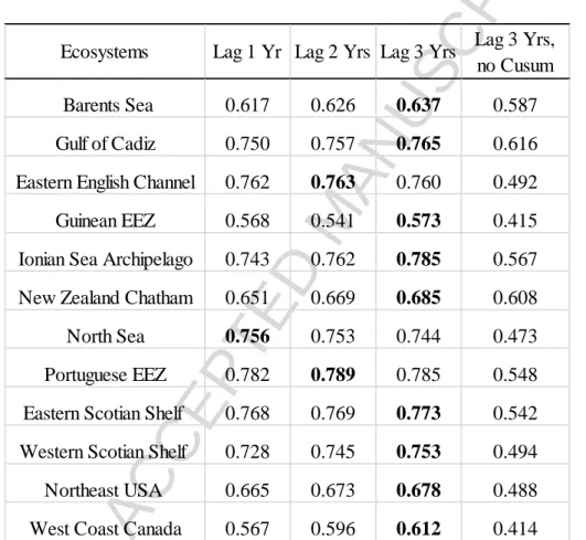
were Cusum-transformed, most ecosystems had GoF values > 0.7, indicating very good model
performances (Table 2). By contrast, non-Cusum transformed data resulted in much lower GoF
values, with only two ecosystems (Gulf of Cadiz and New Zealand Chatham) having GoF > 0.6.
Cusum-transformation thus produces a model more sensitive to consecutive temporal changes,
and more robust to random variations. Hereafter we only present results based on
ACCEPTED MANUSCRIPT
the number of years lagged in the time series did not play a critical role in determining model
performances. We chose a three-year time lag for the rest of analyses, as this produced highest
GoF values for 9 of the 12 ecosystems (Table 2).
With the Cusum-transformed data and three-year time lag for the fisheries exploitation
and environmental condition MVs, we assessed the measurement models for the LVs of fisheryS
and communityS using loadings (correlations between MVs and their underlying LV) and
cross-loadings. Loadings of the seven MVs for the two ecological LVs (fisheryS and communityS)
were generally higher than the cross loadings (Tables D.1, D.2 in Appendix D). This indicated
that the LV fisheryS, consisting of the three catch-based indicators, was inherently different from
the LV communityS, based on the four survey-based indicators. Loadings of fisheryS on its MVs
were generally > 0.7 (seeTables D.1). Three loadings were < 0.7, but still > 0.4.This indicated
that the variances of the catch-based MVs were well explained by fisheryS. While most loadings
of communityS on its MVs were > 0.7, there were five loadings < 0.4 (Table D.2). The MVs
associated with the low loadings included MLife in Guinean EEZ, MLength in North Sea,
MLength in Portuguese EEZ, and MLength and %pred in Northeast USA. Removing these five
MVs improved the GoF by about 3 – 5% in each of the four ecosystems; on the other hand, the
estimates of path coefficients only changed slightly (Table D.3). Values of the average variance
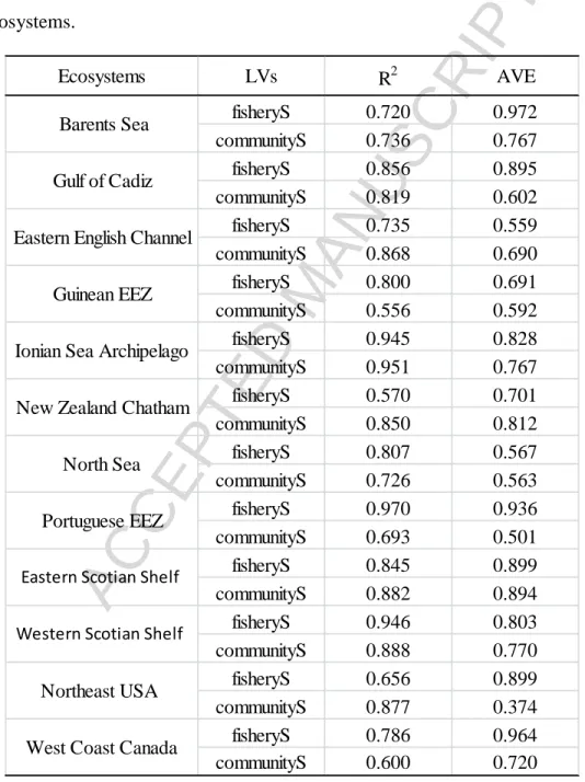
extracted were generally > 0.5 (Table 3), implying that more than half of the variances in MVs
were explained by their corresponding LVs. The R values were generally > 0.7 (Table 3), 2
suggesting that all models had high predictive power.
The addition of the third latent variable resourceP under the structural model Scenario 2
(assuming no direct links with the LVs of fisheries exploitation and environmental conditions)
ACCEPTED MANUSCRIPT
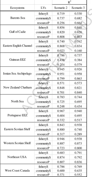
(results not shown) for fisheryS and communityS. However, the R values for resourceP were < 2
0.5 in seven ecosystems, which indicated that the amount of variance in resourceP was not well
explained by fisheryS and communityS in these ecosystems. However, by assuming that direct
links existed between resourceP and the LVs EnvLag, Env0L, ExpLag, and Exp0L in Scenario 3,
we obtained higher R values for 11 ecosystems (Table 4). The assumption of direct links 2
between resourceP and the LVs of fisheries exploitation and environmental conditions allowed
more variance in resourceP to be explained by its independent LVs and thus produced higher
predictive power. This may imply that it is important to account for direct connections when
these direct connections exist. The GoF values were higher for 10 ecosystems under Scenario 3,
although differences were small (Table 5).
3.2 Direct linkages among the LVs
Under the structural model Scenario 1, we examined the relationships between the
independent LVs (EnvLag, Env0L, ExpLag, Exp0L) and the two dependent LVs (fisheryS and
communityS). We focused on the significant correlations. Correlations between fisheryS and the
fisheries exploitation LVs (ExpLag and Exp0L) were either positive (five ecosystems) or
negative (six ecosystems) (Fig. 2, left panel). Positive correlations may imply that periods of
higher fisheries exploitation coincided with periods of fishing at higher trophic levels. In the
eastern Scotian Shelf, exploitation lagged by three-years negatively impacted fisheryS. This
result implied that the higher exploitation three years prior to the indicator response could have
resulted in a shift in fisheries to target species of lower trophic levels or lower vulnerability. In
five ecosystems (Barents Sea, Gulf of Cadiz, Ionian Sea Archipelago, western Scotian Shelf and
West Coast Canada), Exp0L was negatively correlated with fisheryS. These negative correlations
ACCEPTED MANUSCRIPT
species of lower trophic level or less vulnerable species. Effects of environmental conditions on
fisheryS were more likely to be negative (seven ecosystems) than positive (four ecosystems). In
the eastern English Channel and West Coast Canada, both Env0L and EnvLag were negatively
associated with fisheryS; in Northeast USA, both Env0L and EnvLag were positively correlated
with fisheryS.
Significant effects of fisheries exploitation on communityS were caused predominantly
by ExpLag and primarily negative (Fig. 2, right panel). This implies that the negative fishing
effects on the trophic structure and species composition of the surveyed fish community takes
three years to be tracked by ecological indicators. Effects of environmental conditions on
communityS were negative in the Ionian Sea Archipelago, North Sea, eastern Scotian Shelf,
western Scotian Shelf and West Coast Canada. This result suggests that environmental
conditions in these five ecosystems had either negatively affected the whole community,
especially the high trophic level and/or vulnerable species, or had favored species at lower
trophic levels in the past few decades. On the other hand, effects of environmental conditions on
communityS were positive in the Barents Sea, eastern English Channel, New Zealand Chatham,
western and eastern Scotian Shelf.
As we extended the structural model to include the third LV resource in Scenario 2 and
Scenario3, we focused comparisons on path coefficients without considering significant levels
for clearer presentation. Under Scenario 2, previous model diagnoses have indicated that the R2
values were barely changed for fisheryS and communityS compared with Scenario 1 (Table 4 vs.
Table 3). The estimated path coefficients for fisheryS between Scenario 1 and 2 were identical in
terms of direction (i.e., negative or positive) with the exception of Guinean EEZ where the effect
ACCEPTED MANUSCRIPT
changed from positive to negative (Fig. 3). All other differences were minor in the strengths of
the correlations (Fig. 3). Similarly, the direction (i.e., negative or positive) of the estimated path
coefficients for communityS between Scenario 1 and 2 were only different in Northeast USA,
where the effect of Exp0L changed from negative in Scenario 1 to positive in Scenario 2 (Fig. 4).
All other differences between Scenario 1 and 2 were minor in the strengths of the correlations.
Under Scenario 3 assuming direct links between resourceP and the LVs of fisheries
exploitation and environmental conditions, estimated path coefficients were different for some
ecosystems compared to Scenario 2 (Fig. 3). The effect of Exp0L changed from positive in
Scenario 2 to negative in Scenario 3 in Northeast USA; the effect of ExpLag changed from
negative to positive in western Scotian Shelf and it changed from positive to negative in Barents
Sea. Similarly, the estimated path coefficients for communityS were different for some
ecosystems between Scenario 2 and 3. Nevertheless, the general patterns of the path coefficients
remained consistent (Fig. 4).
3.3 Indirect linkages among the LVs
In addition to path coefficients measuring the direct effects of independent LVs on their
dependent LV, PLS-PM also estimates the indirect effect (e.g., the indirect effect of Env0L on
resourceP through either fisheryS or communityS). Fig. A. 4 in Appendix A shows the dissected
total effects EnvLag, Env0L, ExpLag, and Exp0L on resourceP for both Scenario 2 (Fig. A.4i)
and Scenario 3 (Fig. A.4ii) from where a better understanding of the total effects can be
obtained. Fig. 5 shows the total effects of all independent LVs on resourceP for Scenario 2 (left
panel) and Scenario 3 (right penal) for the 12 ecosystems. While the total effects of the fisheries
exploitation LVs (ExpLag and Exp0L) were accounted for as indirect in Scenario 2, they were
ACCEPTED MANUSCRIPT
of both direct and indirect effects in Scenario 3; they became more prominent for all ecosystems.
Similarly, effects of the environmental conditions LVs (EnvLag and Env0L) were more
outstanding in Scenario 3 compared to those in Scenario 2 for most ecosystems (Fig. 5). This
implies that it is important to account for direct effects when there are direct connections
between the independent and dependent LVs, and the indirect effects may not be sufficient to
measure the overall connections. As a result of accounting for the direct connections between
resourceP and the LVs of fisheries exploitation and environmental conditions, the estimated
direct effects of fisheryS or communityS on resourceP in Scenario 3 were smaller than those in
Scenario 2 for most ecosystems (Fig. 5), which suggested weak direct linkages between
resourceP and the ecological LVs of fisheryS and communityS in most ecosystems. Based on
Scenario 3, we found that resourceP was more likely to be associated with communityS than
with fisheryS (Fig. 5, right panel), and the correlations tended to be negative (in eight
ecosystems).
4. Discussion
4.1 Structural model configurations
In this study we have presented a novel application of the Partial Least Squares Path
Modeling approach (PLS-PM) to compare 12 exploited marine ecosystems. This approach
enabled us to quantify the relative effects of fisheries exploitation and environmental and
conditions on ecological indicator responses and explore relationships between indicators and
biomass (i.e., system resource potential).
We investigated three configurations of the structural model: Scenario 1 only including
ACCEPTED MANUSCRIPT
LVs (fisheryS and communityS); Scenario 2 adding the LV of system resource potential
(resourceP) to relate to fisheryS and communityS but assuming no direct effects from the LVs of
fisheries exploitation and environmental conditions on resourceP; and Scenario 3, as an
alternative to Scenario 2, assuming the existence of direct effects of the fisheries exploitation and
environmental conditions on resourceP.
Estimated effects of fisheries exploitation and environmental conditions on fisheryS and
communityS in Scenario 1 barely changed with the addition of resourceP in Scenario 2 where
there were no direct paths from fisheries exploitation and environmental conditions to resourceP.
However, the R values for resourceP were poor (< 0.5) for seven ecosystems, suggesting the 2
variance in resourceP was not well explained by its independent LVs. Allowing resourceP to be
directly influenced by the LVs of fisheries exploitation and environmental conditions in Scenario
3 resulted in higher R values in 11 ecosystems. This indicated that the direct effects of fisheries 2
exploitation and environmental conditions on resourceP were common across the ecosystems
and they should be explicitly modeled if resourceP was to be included in the PLS-PM structural
model. By accounting for these direct connections with fisheries exploitation and environmental
conditions, the direct effects of fisheryS or communityS on resourceP became smaller, which
suggested weaker direct linkages between resourceP and the ecological LVs of fisheryS and
communityS than what were perceived in Scenario 2. In addition, the result also suggested that
the variance in resourceP was better explained by the LVs of fisheries exploitation and
environmental conditions.
In general, comparisons of the estimated effects of fisheries exploitation and
environmental conditions on fisheryS and communityS across the three scenarios revealed that
ACCEPTED MANUSCRIPT
the structural model. As more dependent LVs were added to the structural model for deriving
relationships on a higher order (e.g., resourceP in this case), the estimates of these higher-order
relationships can become sensitive to the configuration of the structural model. Ideally, all
potential configurations of the structural model should be considered and diagnosed in terms of
their predictive power, and the resultant estimates of path coefficients should be compared.
4.2 Grouping ecological indicators
While ecosystem indicators are generally accepted tools for evaluating ecosystem status
and trends (e.g., Shin and Shannon 2010; Shin et al., 2010b; ICES, 2012), it is still unclear how
they can be collectively used for management purposes. With hundreds of ecosystem indicators
having been proposed (Cury and Christensen, 2005; Rochet and Trenkel, 2003; Piet et al., 2008),
the emphasis more recently has been to develop approaches to evaluate and select the most
useful indicators to characterize and monitor ecosystem status in a context of increasing
anthropogenic pressure and climate change (Shannon et al., 2014). Previous work by Shin et al.
(2010b), based on data quality and availability, public awareness and theoretical rationale,
identified the suite of ecological indicators we analyzed here. Shin et al. (2012) recognized that
important selection criteria, such as sensitivity to fishing pressure, time of response, and
specificity of the response to fishing versus climate variability, needed further empirical and
modeling work to assess the usefulness of indicators for ecosystem-based fisheries management.
The current study brings new results to assess these three properties for a set of IndiSeas
indicators across a range of ecosystems.
An earlier study by Link et al. (2010) showed some significant correlations between
individual indicators and environmental and fishing drivers. Here, we used a more complete suite
ACCEPTED MANUSCRIPT
catch-based (fisheryS) or survey-based (communityS). The PLS-PM analysis has shown that
loadings from the seven indicators and their specific LVs were generally larger than cross
loadings for the other LVs, indicating that catch-based and survey-based indicators were
inherently different; and in some ecosystems these two groups of indicators changed in opposite
directions, which is consistent with Shannon et al. (2014). Therefore each group deserved
independent investigation, and both are complementary in terms of quantifying association of
environmental conditions and fisheries exploitation and their subsequent association with the
resource potential. Further, this result indicates that great care should be taken if relying upon a
set of ecological indicators that is derived from one data type only (either catch-based or
survey-based) to characterize ecosystem state.
The grouping of ecological indicators within the PLS-PM provided several valuable
insights: it highlighted associations between groups and relationships among indicators within
each group; it allowed easier interpretation of impacts from environmental and fishing pressures;
and it facilitated connections between indicators and ecosystem attributes, such as biomass (i.e.,
resource potential). This study highlights the utility of the PLS-PM approach in providing a
platform for integrating and simplifying a range of indicators from multiple sources. As
recognized by Murawski (2000), additional sources of indicators (e.g., social and economic) can
provide useful information to evaluate and modify management guidance for important fisheries.
While only two sources of indicators (landings and surveys) have been analyzed here, as a
greater number of indicators are recognized from new sources, additional groupings can be
explored to reflect additional ecosystem attributes.
ACCEPTED MANUSCRIPT
For the effects of fisheries exploitation and environmental conditions on fisheryS and
communityS, we based our comparisons of the 12 ecosystems on Scenario 1, paying special
attention to those that are statistically significant. These estimated effects varied among the
ecosystems both in terms of direction (i.e., negative or positive) and strength, suggesting no
overarching patterns across the ecosystems. Significant correlations between fisheries
exploitation and fisheryS were more common across ecosystems (9 of 12) than those between
fisheries exploitation and communityS. Positive relationships between fisheries exploitation and
fisheryS found in five ecosystems may be interpreted that periods of higher fisheries exploitation
coincided with periods of fishing at higher trophic levels and on more vulnerable species; as
ecosystems were fished down the cascade of trophic levels (Pauly et al., 1998), lower trophic
levels were targeted. Intensive fishing at lower trophic levels is detrimental to an ecosystem,
directly reducing the system biomass (Fu et al., 2013) and increasing ecosystem overexploitation
(Coll et al., 2008), although balanced harvesting, where moderate fishing effort is balanced
across trophic levels or size classes has been shown to maintain ecosystem structure and
productivity (Bundy et al. 2005; Garcia et al., 2012). Therefore, when combined with an
analysis of the historical fishing strategy in an ecosystem, the decreasing trends in these
catch-based indicators could provide warning signs of ecosystem deterioration. However, a keen
knowledge of fisheries management and food web interactions of an ecosystem must be present
before a true warning signal can be recognized since decreasing trends in fisheries exploitation
and FisheryS may also be due to other causes such as redistribution of fishing effort to a more
moderate levels across trophic levels, or to environmental impacts, such as periodically high
ACCEPTED MANUSCRIPT
and reduced allowable catch on higher trophic level fish species, as experienced in the Barents
Sea from 2002-2010 (Johannesen et al., 2012).
It should be noted that the three catch-based MVs were positively correlated only in half
of the 12 ecosystems (Table D.1 in Appendix D). In the other half, one of the three MVs was
negatively correlated with the other two. For instance, IVI was negatively correlated with MTI
and TLc in three ecosystems (eastern English Channel, Ionian Sea Archipelago, and eastern
Scotian Shelf); negative correlations were also observed for MTI in Guinean EEZ, and TLc in
North Sea and Northeast USA. Removing these negative MVs only resulted in slight changes in
estimates of path coefficients (results not shown), thus it would not change the interpretation of
the results. However, the inconsistent correlations between the catch-based indicators for half of
the ecosystems suggested that the assumption of increased fishing pressure resulting in declines
in ecological indicators (Rochet and Trenkel, 2003; Shin et al., 2010b) does not hold universally
(Shannon et al., 2014). How the ecological indicators would change in response to fisheries
exploitation depends on how fisheries operate over time, targeting high or low trophic levels. For
a more complete picture of fisheries exploitation on ecosystem structure and functioning, more
measurements of fishing pressure are needed, although there is no scientific consensus what
these measurements should be. While using component-specific fisheries drivers such as catch
and catch percentage of planktivores and zooplanktivores, Fu et al. (2012) found that these
drivers produced significant responses across all ecosystems and indicators studied. Travers et al.
(2006) also showed that because of indirect effects of fishing on different ecosystem
components, indicators may vary counterintuitively. This is exemplified in various studies
examining trophic level-based indicators, where seemingly unusual trajectories of these
ACCEPTED MANUSCRIPT
accordance with ecosystem type (Cury et al., 2005; Shannon et al., 2010; Shannon et al., 2014),
Therefore, we advocate that fishing configuration (species targeted as well as fishing intensity)
should be incorporated into the development and evaluation of ecological indicators.
Significant effects of fisheries exploitation on communityS were less prevalent in
comparison with fisheryS. It is worth noting that the survey-based MVs of communityS were not
as tightly associated with each other as the catch-based MVs of fisheryS. In particular, there
were five loadings < 0.4 (Table D. 2). This could be due to the survey-based indicators not only
being subject to fisheries exploitation and environmental conditions, but also sampling errors and
ecosystem-specific species composition. The ecosystem-specific species composition may result
in different fishing strategies and subsequently different responses to fisheries exploitation. This
also suggests that exploitation rate and total catch, as measures of fishing pressure, are
insufficient to understand fully the impacts of fisheries exploitation on the ecosystems. Again,
we assert that the fishing configuration should be incorporated into the development and
evaluation of ecological indicators.
Effects of environmental conditions on the ecological LVs were predominantly
significant, and tended to be negative, suggesting that in the recent period, indicators accounted
for changes in environmental conditions and the changes were more likely to be adverse.
However, results presented here might change if we were to apply the approach to different time
periods or to incorporate different environmental variables. In the future, it will be possible to
break down longer times series into periods of sufficient length so that the different impacts of
fisheries exploitation and environmental conditions can be examined and compared between
different time periods for a particular ecosystem.
ACCEPTED MANUSCRIPT
To support the implementation of ecosystem-based approach to fisheries management, it
is important to develop and monitor appropriate indicators of ecosystem status and the
effectiveness of management strategies (Cury and Christensen, 2005; Shin et al., 2010b). It is
challenging to apply traditional statistical approaches such as multiple linear regressions to the
multitude of indicators that are not independent and may contain different or even conflicting
signals and non-linear patterns (Cotter et al., 2009; Petitgas and Poulard, 2009). Our results
clearly show that catch-based and survey-based indicators were inherently different and
sometimes display opposite directions of change. Integrating these two groups of indicators
without careful differentiation will inevitably result in confusing messages when investigating
their responses to environmental changes and fisheries exploitation.
The - PLS-PM approach provides an effective way to separate a multitude of ecosystem
indicators into meaningful groups, each relating to a latent concept. This approach allows the
exploration of the relationships specified between the groups of LVs and their MVs, as well as
relationships among the LVs through an iterative algorithm (Trinchera and Russolillo, 2010). As
we separated ecological indicators into two groups and explored them via the PLS-PM, we were
able to observe relationships of each LV represented by each group of ecological indicators with
fisheries exploitation and environmental conditions. The separation of the catch-based and
survey-based indicators showed that each group related to the resource potential of the
ecosystem differently. Future applications of PLS-PM in fisheries could provide the possibility
of further relating these ecological LVs to management goals through the construction of
management LVs comprised of socio-economic indicators. The advantages and results derived
from our study illustrated the usefulness of PLS-PM for compartmentalizing the multitude of
ACCEPTED MANUSCRIPT
relationships among them. Information derived from these studies will improve our
understanding of ecosystem dynamics and support an ecosystem-based approach to fisheries
management.
Acknowledgements
This is a contribution to the IndiSeas Working Group, endorsed by IOC-UNESCO
(www.ioc-unesco.org) and the European Network of Excellence Euroceans
(www.eur-oceans.eu). The authors would like to thank IndiSeas participants for their contribution in
discussing ideas, objectives, assets and limits of our approach during annual meetings. CF, AB
and JLB were supported by Fisheries and Oceans Canada; YJS, AA and MTT were supported by
the French project EMIBIOS (FRB, contract no. APP-SCEN-2010-II). CPL was supported by
Defra MF1228 (From Physics to Fisheries) and DEVOTES (Development of innovative tools for
understanding marine biodiversity and assessing good Environmental Status) funded by EU FP7
(grant agreement no. 308392), www.devotes-project.eu. All other authors were supported by
their respective affiliations.
References
Alheit, J., Licandro P., Coombs S., Garcia A., Giráldez A., Santamaría M.T.G., Slotte A.,
Tsikliras A.C., 2014. Atlantic Multidecadal Oscillation (AMO) modulates dynamics of
small pelagic fishes and ecosystem regime shifts in the eastern North and Central Atlantic.
ACCEPTED MANUSCRIPT
Bundy, A., Fanning, P., Zwanenburg, K.C.T., 2005. Balancing exploitation and conservation of
the eastern Scotian Shelf ecosystem: application of a 4D ecosystem exploitation index.
ICES Journal of Marine Science 62, 503-510.
Bundy, A., Bohaboy, E.C., Hjermann, D.O., Mueter, F., Fu, C., Link, J.S., 2012. Common
patterns, common drivers: comparative analysis of aggregate surplus production across
ecosystems. Marine Ecology Progress Series 495, 203-218.
Coll M., Shannon L.J., Yemane D., Link J.S., Ojaveer H., Neira S., Jouffre D., Labrosse P.,
Heymans J.J., Fulton E.A., Shin Y.-J., 2010. Ranking the ecological relative status of
exploited marine ecosystems. ICES Journal of Marine Science 67,769–786.
Coll, M., Libralato, S., Tudela, S., Palomera, I. and Pranovi, F., 2008. Ecosystem Overfishing in
the Ocean. PLoS One 3, 1-10.
Conti, L. and Scardi, M., 2010. Fisheries yield and primary productivity in large marine
ecosystems. Marine Ecology Progress Series 410, 233-244.
Cotter, J., Petitgas, P., Abella, A., Apostolaki, P., Mesnil, B., Politou, C.-Y., Rivoirard, J.,
Rochet, M.-J., Spedicato, M.T., Trenkel, V.M., and Woillez, M., 2009. Towards an
ecosystem approach to fisheries management (EAFM) when trawl surveys provide the
main source of information. Aquatic Living Resources 22(02), 243-254.
Cury, P. M. and Christensen, V., 2005. Quantitative ecosystem indicators for fisheries
management. ICES Journal of Marine Science 62(3), 307-310,
doi:10.1016/j.icesjms.2005.02.003
Cury, P., Shannon, L., Roux, J., Daskalov, G., Jarre, A., Moloney, C. and Pauly, D., 2005.
Trophodynamic indicators for an ecosystem approach to fisheries. ICES Journal of Marine
ACCEPTED MANUSCRIPT
Esposito Vinzi, V., Trinchera, L. and Amato, S., 2010. PLS path modeling: from foundations to
recent developments and open issues for model assessment and improvement, in: Esposito
Vinzi, V., Chin, W.W., Henseler, J, Wang, H. (Eds.), Handbook of Partial Least Squares.
Springer: Heidelberg, pp. 47-82.
Fu, C., Gaichas, S., Link, J.S., Bundy, A., Boldt, J.L., Cook, A.M., Gamble, R., Utne, K. R., Liu,
H., Friedland, K.D., 2012. Relative importance of fishing, trophodynamic and
environmental drivers in a series of marine ecosystems. Marine Ecology Progress Series
459, 169-184.
Fu, C., Perry, R.I., Shin, Y.-J., Schweigert, J. and Liu, H., 2013. An ecosystem modelling
framework for incorporating climate regime shifts into fisheries management. Progress in
Oceanography 115, 53-64.
Fulton, E. A., Smith, A. D. M. and Punt, A. E., 2005. Which ecological indicators can robustly
detect effects of fishing? ICES Journal of Marine Science 62, 540-551.
Garcia, S.M., Kolding, J., Rice, J., Rochet, M-J., Zhou, S., Arimoto, T., Beyer, J.E., Borges, L.,
Bundy, A., Dunn, D., Fulton, E.A., Hall, M., Heino, M., Law, R., Makino, M., Rijnsdorp,
A.D., Simard, .F, Smith, A.D.M., 2012. Reconsidering the Consequences of Selective
Fisheries. Science 335, 1045-1047.
Gedalof, Z. and Smith, D.J., 2001. Interdecadal climate variability and regime-scale shifts in
Pacific North America. Geophysical Research Letters 28, 1515-1518.
Götz, O., Kerstin, L.-G. and Krafft, M., 2010. Evaluation of structural equation models using the
partial least squares (PLS) approach, in: Esposito Vinzi, V., Chin, W.W., Henseler, J,
ACCEPTED MANUSCRIPT
Hare, S. R. and Mantua, N. J., 2000. Empirical Evidence for North Pacific Regime Shifts in 1977
and 1989. Progress in Oceanography 47, 103-145.
Ibañez, F., Fromentin, J. M. and Castel, J., 1993. Application de la méthode des sommes
cumulées à l'analyse des séries chronologiques en océanographie. Comptes Rendus de
l'Académie des Sciences de Paris, Sciences de la Vie 316, 745-748.
ICES, 2012. Report of the Working Group on the Ecosystem Effects of Fishing Activities
(WGECO), 11–18 April 2012, Copenhagen, Denmark. ICES CM 2012/ACOM 26, 192 pp.
Jennings, S., 2005. Indicators to support an ecosystem approach to fisheries. Fish and Fisheries
6(3), 212-232.
Jennings, S., Kaiser, M. and Reynolds, J.D., 2001. Marine Fisheries Ecology. Blackwell Science
Ltd.
Johannesen, E. Ingvaldsen, R.B., Bogstad, B., Dalpadado, P., Eriksen, E., Gjøsæter, H., Knutsen,
T., Skern-Maurizten, M., Stiansen, J.E., 2012. Changes in Barents Sea ecosystem state,
1970-2009: climate fluctuations, human impact, and trophic interactions. ICES Journal of
Marine Sciences 69 (5), 880-889.
Kirby, R., Beaugrand, G. and Lindley, J., 2009. Synergistic effects of climate and fishing in a
marine ecosystem. Ecosystems 12(4), 548-561.
Link J.S., Yemane, D., Shannon, L.J., Coll, M., Shin, Y.-J., Hill, L. and Borges, M.F., 2010.
Relating marine ecosystem indicators to fishing and environmental drivers: an elucidation
of contrasting responses. ICES Journal of Marine Science 67, 787–795.
Link, J., 2011. Ecosystem-based fisheries Management: confronting tradeoffs. Cambridge
ACCEPTED MANUSCRIPT
Molinero, J. C., Reygondeau, G. and Bonnet, D., 2013. Climate variance influence on the
non-stationary plankton dynamics. Marine Environmental Research 89, 91-96.
Murawski, S. A., 2000. Definitions of overfishing from an ecosystem perspective. ICES Journal
of Marine Science 57(3), 649-658.
Pauly, D., Christensen, V., Dalsgaard, J., Froese, R. and Torres Jr., F., 1998. Fishing Down
Marine Food Webs. Science 279 (5352), 860-863.
Petitgas, P. and Poulard, J.-C., 2009. A multivariate indicator to monitor changes in spatial
patterns of age-structured fish populations. Aquatic Living Resources 22(02), 165-171.
Piet, G.J., Jansen, H.M. and Rochet, M.-J., 2008. Evaluating potential indicators for an
ecosystem approach to fishery management in European waters. ICES Journal of Marine
Science 65(8), 1449-1455.
R Development Core Team, 2013. R: A language and environment for statistical computing. R
Foundation for Statistical Computing, Vienna, Australia. WWW page,
http://www.R-project.org/ Latest access: 09 May 2014.
Rice J.C., Rochet M.-J., 2005. A framework for selecting a suite of indicators for fisheries
management. ICES Journal of Marine Science 62, 516–527.
Rochet, M.-J. and Trenkel, V. M., 2003. Which community indicators can measure the impact of
fishing? A review and proposals. Canadian Journal of Fisheries and Aquatic Sciences 60,
86-99.
Rochet, M.-J. and Trenkel, V., 2009. Why and How Could Indicators Be Used in an Ecosystem
Approach to Fisheries Management? Fish and Fisheries Series 31, 209-226.
Rouyer, T., Fromentin, J.-M., Ménard, F., Cazelles, B., Briand, K., Pianet, R., Planque, B. and
ACCEPTED MANUSCRIPT
forcing, and exploitation in fisheries. Proceedings of the National Academy of Sciences
105(14), 5420-5425.
Sanchez, G., 2013. PLS Path Modeling with R. WWW page,
http://www.gastonsanchez.com/PLS Path Modeling with R.pdf Downloaded on 02
November 2013.
Samhouri, J., Levin, P., and Harvey, C., 2009. Quantitative evaluation of marine ecosystem
indicator performance using food web models. Ecosystems 12(8), 1283-1298.
Shannon, L.J., Coll, M., Yemane, D., Jouffre, D., Neira, S., Bertrand, A., Diaz, E. & Shin, Y.-J.,
2010. Comparing data-based indicators across upwelling and comparable systems for
communicating ecosystem states and trends. ICES Journal of Marine Science 67, 807–832.
Shannon, J.L., Coll, M., Bundy, A., Gascuel, D., Heymans, J.J., Kleisner, K., Lynam, C.P.,
Piroddi, C., Tam, J., Travers-Trolet, M. & Shin, Y.J., 2014. Trophic level-based indicators
to track fishing impacts across marine ecosystems. Marine Ecology Progress Series 512,
115-140.
Shin, Y.-J. and Shannon, L. J., 2010. Using indicators for evaluating, comparing and
communicating the ecological status of exploited marine ecosystems. 1. The IndiSeas
project. ICES Journal of Marine Science 67, 686–691.
Shin, Y.-J., Shannon, L. J., Simier, M., Coll, M., Fulton, E. A., Link, J. S., Jouffre, D., Ojaveer,
H., Mackinson, S., Heymans, J. J., Raid, T. 2010a. Can simple be useful and reliable?
Using ecological indicators to represent and compare the states of marine ecosystems.
ICES Journal of Marine Science, 67:717–731.
Shin, Y.-J., Shannon, L. J., Bundy, A., Coll, M., Aydin, K., Bez, N., Blanchard, J. L., Borges, M.
ACCEPTED MANUSCRIPT
Labrosse, P., Link, J.S., Mackinson, S., Masski, H., Möllmann, C., Neira, S., Ojaveer, H.,
ould Mohammed Abdallahi, K., Perry, I., Thiao, D., Yemane, D. & Cury, P.M., 2010b.
Using indicators for evaluating, comparing, and communicating the ecological status of
exploited marine ecosystems. 2. Setting the scene. ICES Journal of Marine Science 67,
692-716.
Sissenwine, M. and Murawski, S., 2004. Moving beyond ‘intelligent thinking’: advancing an
ecosystem approach to fisheries. Marine Ecology Progress Series 274, 291-295.
Travers, M, Shin, Y-J, Shannon, L. and Cury, P., 2006. Simulating and testing the sensitivity of
ecosystem-based indicators to fishing in the southern Benguela ecosystem. Canadian Journal
of Fisheries and Aquatic Sciences 63, 943-956.
Trinchera, L. and Russolillo, G., 2010. On the use of Structural Equation Models and PLS Path
Modeling to build composite indicators. University of Macerata, Italy.
Ware, D.M. and Thomson, R.E., 2005. Bottom-up ecosystem trophic dynamics determine fish
production in the Northeast Pacific. Science 308, 1280-1284.
Wells, B., Field, J., Thayer, J., Grimes, C., Bograd, S., Sydeman W., Schwing F. & Hewitt, R.,
2008. Untangling the relationships among climate, prey and top predators in an ocean
ecosystem. Marine Ecology Progress Series 364, 15-29.
Wold, H., 1980. Model construction and evaluation when theoretical knowledge is scarce: On
the theory and application of Partial Least Squares, in: Kmenta, J., Ramsey, J. (Eds.),
Model Evaluation in Econometrics. Academic Press, New York, pp. 47-74.
Zuur, A.F., Ieno, E.N. and Elphick, C.S., 2010. A protocol for data exploration to avoid common
statistical problems. Methods in Ecology and Evolution 1(1), 3-14.
ACCEPTED MANUSCRIPT
Table 1. Local- and basin-scale environmental variables analyzed in the 12 ecosystems for the
given periods: NAO (North Atlantic Oscillation index), AMO (Atlantic Multidecadal
Oscillation index), EAP (East Atlantic Pattern), MOI (Mediterranean Oscillation Index),
SST (Sea Surface Temperature), SAM (Southern Annular Mode), SOI (Southern Oscillation
Index) and PDO (Pacific Decadal Oscillation).
Ecosystems Start year End year Local 1 Local 2 Local 3 Basin 1 Basin 2
Barents Sea 1983 2010 Ice cover
Average temperature at 50-200 m
- NAO AMO
Gulf of Cadiz 1993 2010 River
discharge - - NAO AMO
Eastern English Channel 1988 2010 SST - - NAO AMO
Guinean EEZ 1985 2009 SST - - NAO AMO
Ionian Sea Archipelago 1964 2007 SST - - MOI
-New Zealand Chatham 1993 2010 - - - PDO SAM
North Sea 1983 2010 SST - - NAO AMO
Portuguese EEZ 1980 2010 - - - NAO EAP
Eastern Scotian Shelf 1970 2010 SST Stratification index
Temperature
at 100m NAO
-Western Scotian Shelf 1970 2010 SST Stratification index
Temperature
at 100m NAO
-Northeast USA 1964 2010 Wind stress River
discharge - NAO AMO
West Coast Canada 1980 2010 Upwelling index
Transport
ACCEPTED MANUSCRIPT
Table 2. Goodness of fit values under four scenarios: time series were Cusum transformed and
the time lagged latent variables (LVs) of fisheries exploitation and environmental conditions
have lags of one to three years, as well as a fourth scenario without the Cusum
transformation and with a lag of three years. The highest goodness of fit value is in bold for
each ecosystem.
Ecosystems Lag 1 Yr Lag 2 Yrs Lag 3 Yrs Lag 3 Yrs,
no Cusum
Barents Sea 0.617 0.626 0.637 0.587
Gulf of Cadiz 0.750 0.757 0.765 0.616
Eastern English Channel 0.762 0.763 0.760 0.492
Guinean EEZ 0.568 0.541 0.573 0.415
Ionian Sea Archipelago 0.743 0.762 0.785 0.567
New Zealand Chatham 0.651 0.669 0.685 0.608
North Sea 0.756 0.753 0.744 0.473
Portuguese EEZ 0.782 0.789 0.785 0.548
Eastern Scotian Shelf 0.768 0.769 0.773 0.542
Western Scotian Shelf 0.728 0.745 0.753 0.494
Northeast USA 0.665 0.673 0.678 0.488
ACCEPTED MANUSCRIPT
Table 3. Values of R (representing predictive power of the model) and average variance 2
extracted (AVE) for the two latent variables (fisheryS: structure of landed fish, communityS:
structure of the surveyed fish community) under structural model Scenario 1 for the 12
ecosystems. Ecosystems LVs R2 AVE fisheryS 0.720 0.972 communityS 0.736 0.767 fisheryS 0.856 0.895 communityS 0.819 0.602 fisheryS 0.735 0.559 communityS 0.868 0.690 fisheryS 0.800 0.691 communityS 0.556 0.592 fisheryS 0.945 0.828 communityS 0.951 0.767 fisheryS 0.570 0.701 communityS 0.850 0.812 fisheryS 0.807 0.567 communityS 0.726 0.563 fisheryS 0.970 0.936 communityS 0.693 0.501 fisheryS 0.845 0.899 communityS 0.882 0.894 fisheryS 0.946 0.803 communityS 0.888 0.770 fisheryS 0.656 0.899 communityS 0.877 0.374 fisheryS 0.786 0.964 communityS 0.600 0.720 Northeast USA
West Coast Canada New Zealand Chatham
North Sea
Portuguese EEZ
Eastern Scotian Shelf
Western Scotian Shelf
Barents Sea
Gulf of Cadiz
Eastern English Channel
Guinean EEZ
ACCEPTED MANUSCRIPT
Table 4. Comparisons of R values (representing predictive power of the model) and average 2
variance extracted (AVE) for the three latent variables (fisheryS: structure of landed fish, communityS: structure of the surveyed fish community, and resourceP: resource potential reflected by total biomass) under Scenario 2 of the structural model (without direct link between resourceP and the LVs of fisheries exploitation and environmental conditions) and Scenario 3 (with direct link) for the 12 ecosystems.
Ecosystems LVs Scenario 2 Scenario 3
fisheryS 0.719 0.530 communityS 0.737 0.682 resourceP 0.256 0.664 fisheryS 0.856 0.840 communityS 0.820 0.820 resourceP 0.808 0.863 fisheryS 0.740 0.762 communityS 0.868 0.834 resourceP 0.023 0.160 fisheryS 0.786 0.737 communityS 0.438 0.384 resourceP 0.214 0.579 fisheryS 0.945 0.926 communityS 0.951 0.958 resourceP 0.799 0.863 fisheryS 0.571 0.573 communityS 0.848 0.821 resourceP 0.701 0.840 fisheryS 0.783 0.744 communityS 0.725 0.695 resourceP 0.248 0.434 fisheryS 0.967 0.940 communityS 0.604 0.695 resourceP 0.332 0.517 fisheryS 0.843 0.938 communityS 0.880 0.740 resourceP 0.317 0.289 fisheryS 0.946 0.938 communityS 0.887 0.873 resourceP 0.723 0.800 fisheryS 0.683 0.791 communityS 0.874 0.792 resourceP 0.807 0.836 fisheryS 0.786 0.769 communityS 0.600 0.635 resourceP 0.371 0.552 Northeast USA
West Coast Canada Ionian Sea Archipelago
New Zealand Chatham
North Sea
Portuguese EEZ
Eastern Scotian Shelf
Western Scotian Shelf
R2
Barents Sea
Gulf of Cadiz
Eastern English Channel
ACCEPTED MANUSCRIPT
Table 5. Goodness of fit values for the 12 ecosystems under Scenario 2 of the structural model (without direct link between resourceP and the LVs of fisheries exploitation and
environmental conditions) and Scenario 3 (with direct link).
Ecosystems Scenario 2 Scenario 3
Barents Sea 0.585 0.632
Gulf of Cadiz 0.778 0.782
Eastern English Channel 0.638 0.662
Guinean EEZ 0.507 0.562
Ionian Sea Archipelago 0.788 0.794
New Zealand Chatham 0.703 0.724
North Sea 0.663 0.679
Portuguese EEZ 0.696 0.720
Eastern Scotian Shelf 0.699 0.657
Western Scotian Shelf 0.747 0.756
Northeast USA 0.706 0.706
ACCEPTED MANUSCRIPT
Figure CaptionsFigure 1. Diagram of the partial least squares path model, showing in dashed arrows
relationships among latent variables (LVs) of environment (Env) and fisheries exploitation
(Exp), trophic structure and species composition of landings (fisheryS) and of the surveyed
fish community (commnityS), as well as system resource potential. Each of the LVs is
related to its own manifest variables (MVs) shown as solid arrows: the LV Env is related to
three local variables (LI1, LI2, and LI3) and two basin-scale variables (BS1 and BS2), and
the LV Exp is related to total landings (totalC) and exploitation rate (exp); fisheryS is
reflected by marine trophic index (MTI), mean trophic level of landings (TLc), and intrinsic
vulnerability index of landings (IVI), and communityS by mean length (MLength), mean life
span (MLife), trophic level (TLco) and proportion of predatory fish (%pred) in the
community; system resource potential is represented by the total biomass time series
(totalB). For simplicity, LVs with lagged times series are not shown.
Figure 2. Path coefficients for the latent variables (LVs) fisheryS (representing the structure of
landings, left panel) and communityS (the structure of the surveyed fish community, right
panel) in relation to the LVs of fisheries exploitation and environmental conditions without
time lags (Env0L and Exp0L) and with time lags of three years (EnvLag and ExpLag).
Statistically significant (p<0.05) path coefficients are shown in bright colors and
non-significant ones in grey.
Figure 3. Estimated path coefficients for the eight pathways of the latent variable fisheryS that
are common to the three scenarios of the structural model: (1) Scenario 1 does not have the
LV resourceP (representing resource potential); (2) Scenario 2 has the LV resourceP but
ACCEPTED MANUSCRIPT
environmental condition; (3) Scenario 3 has resourceP and assumes direct links between
resourceP and the LVs of fisheries exploitation and environmental conditions.
Figure 4. Estimated path coefficients for the eight pathways of the latent variable communityS
that are common to the three scenarios of the structural model: (1) Scenario 1 does not have
the LV resourceP (representing resource potential); (2) Scenario 2 has the LV resourceP but
assumes no direct links between resourceP and the LVs of fisheries exploitation and
environmental condition; and (3) Scenario 3 has resourceP and assumes direct links between
resourceP and the LVs of fisheries exploitation and environmental condition.
Figure 5. Total effects on the latent variable (LV) resourceP (representing resource potential)
from the LVs fisheryS and communityS and the environmental and fisheries exploitation
LVs (EnvLag, Env0L, ExpLag, Exp0L) under two scenarios: (1) Scenario 2 assumes no
direct links between resourceP and the LVs of fisheries exploitation and environmental
condition; and (2) Scenario 3 assumes direct links between resourceP and the LVs of
fisheries exploitation and environmental condition. Notice the scale differences between
ACCEPTED MANUSCRIPT
Fig. 1