Deciphering the developmental plasticity of walnut saplings in relation to climatic factors and light environment

HAL Id: hal-00828855

https://hal.inria.fr/hal-00828855

HAL is a multi-disciplinary open access archive for the deposit and dissemination of sci-entific research documents, whether they are pub-lished or not. The documents may come from teaching and research institutions in France or abroad, or from public or private research centers.

L’archive ouverte pluridisciplinaire HAL, est destinée au dépôt et à la diffusion de documents scientifiques de niveau recherche, publiés ou non, émanant des établissements d’enseignement et de recherche français ou étrangers, des laboratoires publics ou privés.

Deciphering the developmental plasticity of walnut

saplings in relation to climatic factors and light

environment

Olivier Taugourdeau, Florence Chaubert-Pereira, Sylvie Sabatier, Yann

Guédon

To cite this version:

Olivier Taugourdeau, Florence Chaubert-Pereira, Sylvie Sabatier, Yann Guédon. Deciphering the developmental plasticity of walnut saplings in relation to climatic factors and light environment. Journal of Experimental Botany, Oxford University Press (OUP), 2011, 62 (15), pp.5283-5296. �10.1093/jxb/err115�. �hal-00828855�

Deciphering the developmental plasticity of walnut saplings in

relation to climatic factors and light environment

1 2 3 4 5 6 7 8 9 10 11

Olivier Taugourdeau1, Florence Chaubert-Pereira2, Sylvie Sabatier1, Yann Guédon2*

1

CIRAD/UM2, UMR botAnique et bioinforMatique de l’Architecture des Plantes, TA A-51/PS2, 34398 Montpellier Cedex 5, France (olivier.taugourdeau@cirad.fr, sylvie-annabel.sabatier@cirad.fr)

2

CIRAD, UMR Amélioration Génétique et Adaptation des Plantes méditerranéennes et tropicales and INRIA, Virtual Plants, TA A-96/02, 34398 Montpellier Cedex 5, France (chauchau64@gmail.com, guedon@cirad.fr) 12 13 14 15 16 17 18 19 20 21 22 23 24 25

*Corresponding author: guedon@cirad.fr,

5 Tables, 7 Figures

Running title: Developmental plasticity of walnuts saplings

Abstract

Developmental plasticity, the acclimation of plants to their local environment, is known to be crucial for the fitness of perennial organisms such as trees. However, deciphering the many possible developmental and environmental influences involved in such plasticity in natural conditions requires dedicated statistical models integrating developmental phases, environmental factors and inter-individual heterogeneity. These models should be able to analyze retrospective data (number of leaves or length of annual shoots along the main stem in our case). In this study Markov switching linear mixed models were applied to the analysis of the developmental plasticity of walnut saplings during the establishment phase in a mixed

1 2 3 4 5 6 7 8 9 10 11 12 13 14 15 16 17 18 19 20 21 22 23 24 25

Mediterranean forest. In the Markov switching linear mixed models estimated from walnut data sets, the underlying Markov chain represents both the succession and lengths of growth phases, while the linear mixed models represent both the influence of climatic factors and inter-individual heterogeneity within each growth phase. On the basis of these integrative statistical models, it is shown that walnut saplings have an opportunistic mode of development that is primarily driven by the changing light environment. In particular, light availability explains the ability of a tree to reach a phase of strong growth where the first branches can appear. It is also shown that growth fluctuation amplitudes in response to climatic factors increased while inter-individual heterogeneity decreased along tree development.

Key words: growth components; Juglans regia L.; linear mixed model; Markov switching model; ontogeny; plant architecture.

Introduction

In natural conditions the developmental plasticity of trees is one of the main determinants of forest successional dynamics. In particular, the early life period to a large extent conditions the modalities of replacement of senescent trees by young trees. In understory, tree growth is driven by light availability with substantial differences according to shade tolerance (Wright et

al., 2000) and climatic factors (Sanchez-Gomez et al., 2008). Here, our objective was to study

the establishment phase of trees by focusing on apical growth and branching of young trees growing in a mixed forest. One of the major difficulties when studying developmental plasticity is the “real-world complexity of multiple biotic and abiotic variables” (Miner et al., 2005). Hence a decomposition approach should be applied to identify and characterize the different variables that influence tree development.

1 2 3 4 5 6 7 8 9 10 11 12 13 14 15 16 17 18 19 20 21 22 23 24 25

Tree structure development can be reconstructed at a given observation date from external morphological markers (such as cataphyll and branching scars) that correspond to past events (Barthélémy and Caraglio, 2007). Observed apical growth, as given for instance by the length of successive annual shoots along a tree main stem, is assumed to result mainly from three components: an ontogenetic component, an environmental component and an individual component (Chaubert-Pereira et al., 2009). The ontogenetic component is assumed to be structured as a succession of roughly stationary growth phases that are asynchronous between individuals (Guédon et al., 2007). A phase is said to be stationary if there is no systematic change in mean (no trend), no systematic change in variance and no strictly periodic variation of the variable of interest. The key question tackled in Guédon et al. (2007) was whether the ontogenetic growth component along an axis at the growth unit or annual shoot scale takes the form of a trend (i.e. a gradual change in the mean level) or of a succession of phases. Their results support the assumption of abrupt changes between roughly stationary phases rather than gradual changes. The environmental component is assumed to take the form of local fluctuations that are synchronous between individuals. This environmental component is thus assumed to be a “population” component as opposed to the individual component which represents the growth level deviation in each phase of a tree with reference to the “average” tree. The individual component may cover effects of diverse origins but always includes a genetic effect (Sabatier et al., 2003a; Segura et al., 2008). Other effects correspond to the tree's local environment (e.g. light resources); see Pinno et al. (2001) and Dolezal et al. (2004).

Here, we propose to use Markov switching linear mixed models (Chaubert-Pereira et al., 2010) to analyze growth components of walnut saplings. In a Markov switching linear mixed model, the underlying Markov chain represents both the succession and lengths of growth phases, while the linear mixed models attached to each state of the Markov chain represent both the

1 2 3 4 5 6 7 8 9 10 11 12 13 14 15 16 17 18 19 20 21 22 23 24 25

effect of time-varying climatic explanatory variables and inter-individual heterogeneity. The effect of climatic explanatory variables is modeled as a fixed effect and inter-individual heterogeneity as a random effect. Thus, the introduction of random effects makes it possible to decompose the total variability into two parts: variability due to inter-individual heterogeneity and residual variability. In this study, Markov switching models were identified using semi-Markov switching models, a more general family of models that encompasses as particular cases Markov switching models. In a semi-Markov switching model, the length of each growth phase is explicitly modeled by a dedicated parametric discrete distribution (Chaubert-Pereira et

al., 2009) while in a Markov switching model, the length of each growth phase is implicitly

modeled by a geometric distribution, which is the unique “memoryless” discrete distribution. This led us to contrast the development of saplings in understory with the development of trees in managed forest stands studied by Chaubert-Pereira et al. (2009).

Markov switching linear mixed models were applied to the analysis of successive annual shoots along walnut main stems using two possible response variables, namely (i) the number of leaves per annual shoot corresponding to organogenesis alone and (ii) annual shoot length, corresponding to organogenesis and elongation, and two climatic explanatory variables, namely (i) average daily maximum temperature and (ii) cumulative rainfall. The building of two models, one corresponding to organogenesis alone and the other corresponding to organogenesis and elongation can be viewed as a way to refine the decomposition of tree growth that is intrinsic to Markov switching linear mixed models. Light environments were also compared for four tree categories deduced from the statistical modeling. The objective was to study the relationship between the architecture of these juvenile trees growing in a mixed Mediterranean forest and the two selected climatic factors and the local light environment.

1 2 3 4 5 6 7 8 9 10 11 12 13 14 15 16 17 18 19 20 21 22 23 24 25

The aim of this study was to assess the effects of the environment on understory saplings development. In this study, the ontogeny was viewed as “a developmentally programmed growth trajectory preadjusted to the most likely environments; the surrounding environments mainly affect the rate at which saplings move along this trajectory.” (Yagi, 2009). Two main hypotheses were tested: (i) unfavorable light environment delays tree ontogeny but without impacting growth potential and, (ii) The effects of climatic factors depend on the ontogenetic stage.

Materials and methods

Materials

Study site

The studied stand was a Mediterranean mixed forest located near Montpellier (43°40'33'' N; 3°51'53'' E) in the south of France. Mean stand elevation is 57 m and the climate is typically Mediterranean (dry summer, rainfall mainly in autumn and spring) with mean annual cumulative rainfall of 732 mm, an annual mean daily maximum temperature of 20.2°C and an annual mean daily minimum temperature of 9.4°C for the period 1977-2006. The forest canopy mainly consisted of crowns of Quercus ilex L., Quercus pubescens Willd., Pinus halepensis Mill. and Tilia platyphyllos Scop.. The understory consisted of saplings of Q. ilex, Q. pubescens,

T. platyphyllos, Celtis australis L., Prunus avium L., and Juglans regia L.. Hedera helix L. and Ruscus aculeatus L. covered the ground. The transmitted light, i.e. the percentage of incident

radiations not intercepted by the canopy, ranged from 5 to 35 % in the studied understory.

Tree data set

1 2 3 4 5 6 7 8 9 10 11 12 13 14 15 16 17 18 19 20 21 22 23 24 25

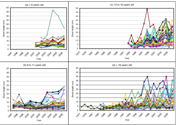
(see Figs. 1 and 2). Since only one mother tree was present at the edge of the studied stand, we suspect that most of the saplings were half-brothers. The successive annual shoots along the main stems were entirely preformed, i.e. all the organs of the next-year elongated shoot were present at an embryonic stage in the winter bud. The limit between two successive annual shoots is marked by a zone of short internodes and scale leaves (Sabatier and Barthélémy, 2001) which facilitates the retrospective measurement of successive annual shoots along the main stem. In March 2007 before bud break, the main stems of the trees were described by annual shoot and three quantitative variables were recorded for each annual shoot: number of leaves (between 2 to 12), length in cm (between 1 and 49 cm; see Figs. 1 and 2) and number of branches. Of the 138 trees measured, 22 were branched. The measured trees were between 3 and 31 years old. All these trees were in the juvenile phase (i.e. before the first flowering occurrence) the last year considered.

The very first annual shoot corresponding to the germination year was not included in the analysis as it is far longer than the subsequent annual shoots and its length (range: 2-53 cm; mean: 20.22 cm; standard deviation: 6.54 cm) is greatly dependent on seed mass. The correlation coefficients between the length of this very first annual shoot and the length of each of the five subsequent annual shoot were not significantly different from 0 (as well as between the length of this very first annual shoot and the cumulative length of the - from two to five - subsequent annual shoots). Hence, the length of this first annual shoot was not related to subsequent tree development. This can be interpreted as the fact that the local environment had a far stronger effect on the sapling development after the first year of growth than the seed mass. After the germination year, the length of successive annual shoots increased along the main stem. Individuals showed synchronous inter-annual fluctuations the amplitude of which was roughly proportional to the growth level (i.e. average shoot length within a phase) (Fig. 1).

1 2 3 4 5 6 7 8 9 10 11 12 13 14 15 16 17 18 19 20 21 22 23

These inter-annual fluctuations were thus assumed to be mainly of climatic origin.

Meteorological data set

Data for daily maximum temperature (°C) and cumulative rainfall (in mm) were provided by INRA-Montpellier (Lavalette site, a nearby meteorological field station) for the period from 1977 to 2006 (the last year considered).

Measuring light and leaf mass area

Light availability in the understory was quantified by hemispherical photography. Photographs were taken in May 2007 after leaf expansion of canopy species, above the terminal bud of the main stem of each studied tree. The photographs were taken using a horizontally-leveled digital camera (CoolPix 8400, Nikon) mounted on a tripod and aimed at the zenith. A fish-eye lens providing a 180° field of view was employed (Coolpix FC-E9, Nikon). These photographs were analyzed for canopy openness (i.e. percentage of open sky) and percentage of light transmitted by the forest canopy during the growing season (i.e. April-October) using GLA2 software (Frazer et al., 1999). Theses two indicators are commonly used to compare sapling light environments (Kobe and Hogarth, 2007).

Leaf dry mass per unit leaf area (LMA) was computed from a 5 cm2 piece of lamina (i.e.

without the leaflet midrib) taken from one leaflet per tree. These leaflets were sampled in similar positions within the 2007 main stem shoot. This sampling was completed in a single two-hour period during the 2007 summer. LMA computed in this manner is generally considered as a reliable indicator of leaf structure (Niinemets 1999).

Markov and semi-Markov switching linear mixed models 1 2 3 4 5 7 10 11 12 13 14 15 16

In the analysis we considered two possible tree response variables: (i) the number of leaves per annual shoot and (ii) the length of the annual shoot in cm. In cases where climatic explanatory variables are available, a statistical model for analyzing this type of tree growth data should be able to model jointly:

- the succession of roughly stationary growth phases that are asynchronous between 6

individuals,

- the effect of time-varying climatic explanatory variables, 8

- inter-individual heterogeneity. 9

We therefore chose to build Markov switching linear mixed models. This family of statistical models broadens the family of Markov switching linear models; see Frühwirth-Schnatter (2006) for an overview of Markov switching models. A Markov switching linear mixed model combines:

- a non-observable J-state Markov chain which represents the succession of growth phases and their lengths where each state of the Markov chain represents a growth phase. A J-state Markov chain is defined by two subsets of parameters:

1. Initial probabilities

(

)

in the sequence measured for a tree, 17

18

2. Transition probabilities

(

)

phases and their lengths along the main stem. 19 20 21 22 23 24

- J linear mixed models, each one attached to a state of the underlying Markov chain. Each linear mixed model represents, in the corresponding growth phase, both the effect of time-varying climatic explanatory variables as fixed effects and inter-individual

1 2 3 4 5

heterogeneity as a random effect; see Verbeke and Molenberghs (2000) for an overview of linear mixed models applied to longitudinal data.

The observed annual shoot length for tree a being in state j at year t is modeled by the

following linear mixed model:

t a Y , , , , , 3 3 , 2 2 1 ,t j j t j t j a j at a X X Y =β +β +β +τ ξ +ε 6 7 where:

- β_j1+β_j2X_2,t +β_j3X_3,t is the contribution of the fixed effects for state j, β_j1 the intercept

which represents the average growth level, 8

2

j

β the regression parameter for average daily

maximum temperature, the average daily maximum temperature common to all the trees

that is relevant for year t, 9

10 X_2,t

3

j

β the regression parameter for cumulative rainfall, the

cumulative rainfall common to all the trees that is relevant for year t. It should be noticed that the tree response to time-varying climatic factors is most often delayed and “smoothed”.

t X3,

11 12 13

-

ξ

τ

deviation induced by the inter-individual heterogeneity in state j. The random effects are

assumed to follow the standard Gaussian distribution . Individual tree status is assumed

to be different in each growth phase. For a given individual, the average shoot length within a phase can be higher than that of the “average tree” then lower in the following phase.

14 15 16 17 18 19 20 21 22 23 ) 1 , 0 ( N

- is the error term corresponding to tree a being in state j at year t

and is the residual variance.

) , 0 ( N ~ | , 2 ,t at j a S j

σ

ε

When considering the number of leaves per annual shoot, the linear mixed model is similar except for the cumulative rainfall fixed effect which is not incorporated; see the Results for

justifications. The introduction of random effects makes it possible to decompose the total

variability in state j into two parts:

1 2 3 4 5 6 7 8 9 10 11 12 13 14 15 16 17 18 19 2 j Γ 2 2 2 j j j =τ +σ Γ ,

where is the variability due to inter-individual heterogeneity and is the residual

variability. The proportion of inter-individual heterogeneity is defined by the ratio between the

random effect variance and the total variance .

2 j τ 2 j σ 2 j τ 2 j Γ

Markov switching linear mixed models were estimated using a Monte Carlo expectation maximization (MCEM)-like algorithm (Chaubert-Pereira et al., 2010). At convergence of the iterative estimation algorithm, the median predicted random effects were computed for each individual based on the random effects predicted for each state in each sampled state sequence. The most probable state sequence given the median predicted random effects was computed for each observed sequence using a Viterbi-like algorithm. This restored state sequence can be considered as the optimal segmentation of the corresponding observed sequence into sub-sequences, each corresponding to a given growth phase.

Standard errors for the regression parameters of Markov switching linear mixed models were computed using a Monte Carlo version of the Louis method (Chaubert-Pereira et al., 2010). In our case of non-ergodic models (a model is said to be ergodic if each state is visited many

times), we chose also to compute βjk×madj(Xk) for each state j where is the

mean absolute deviation of the climatic explanatory variable k in state j. This indicator gives empirical evidence of the significant or non-significant character of the corresponding climatic effect. ) ( madj Xk 20 21 22 23 24

A useful generalization of Markov switching linear mixed models lies in the class of semi-Markov switching linear mixed models (Chaubert-Pereira et al., 2010) where the underlying Markov chain is replaced by an underlying semi-Markov chain. In a semi-Markov chain, the process moves out of a given state according to a Markov chain with self-transition probability in nonabsorbing states 1 2 3 4 0 ~ =_ii p ij p

. This embedded Markov chain represents transitions between distinct states except in the absorbing state case. A state is said to be absorbing if, after entering this state, it is impossible to leave it. An explicit occupancy (or sojourn time) distribution is attached to each nonabsorbing state to model the growth phase length in number of years. The whole (embedded Markov chain + explicit state occupancy distributions) constitutes a semi-Markov chain. The mechanism associated with a semi-semi-Markov chain can be described as follows: suppose that between two consecutive times, a transition occurred between state i and state j with probability

5 6 7 8 9 10 11

~ . The process remains in state j for a period u determined randomly by the corresponding state occupancy distribution

12

( )

{

}

another state according to the transition distribution attached to state j 13

(

)

14 15 16 17 18 19 20 21 22 23 24

Results

Choice of climatic explanatory variables

In walnut, organogenesis occurs from early April to late May of the previous year and organ elongation occurs the current year during the same period (Sabatier et al., 2003b). We chose to build two statistical models, the first corresponding to organogenesis alone where the tree

response variable is the number of leaves per annual shoot, and the second corresponding to organogenesis and elongation where the tree response variable is the annual shoot length. Since both the number of leaves and the length of successive annual shoots increased along the main stem (Fig. 1), these variables could not be considered as stationary and non-ergodic models, in our case “left-right” models (see below), were built. We chose to use average daily maximum temperature and cumulative rainfall and to center these climatic explanatory variables; see Fitzmaurice et al. (2004) for discussion of the centering issue. Because of the centering, the intercept 1 2 3 4 5 6 7 1 j

β is directly interpretable as the average number of leaves per annual shoot in

growth phase j. In a first step, we tested different climatic explanatory variables for the “number of leaves” model. We did not identify a significant cumulative rainfall effect for this model whatever the period tested. The maximum temperature explanatory variable selected for the “number of leaves” model was then incorporated in the “annual shoot length” model and other climatic explanatory variables were tested in a second step for this model.

8 9 10 11 12 13 14 15 16 17 18 19 20 21 22 23 24 25

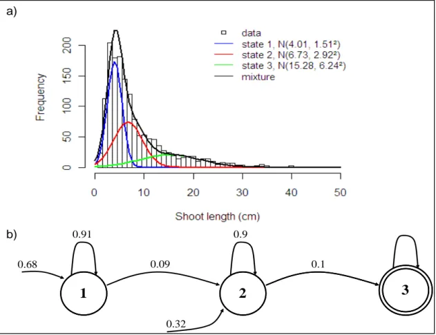
In order to determine the most significant period for average daily maximum temperature, a “left-right” three-state Markov switching linear model (i.e. without random effects for modeling inter-individual heterogeneity) composed of two transient states followed by a final absorbing state was first estimated for different periods covering the organogenesis period on the basis of the number of leaves per annual shoot; see below for the choice of the number of states of the underlying Markov chain. A state is said to be transient if after leaving this state it is impossible to return to it. In a “left-right” model, the states are therefore ordered and each state can be visited at most once. In this sensitivity analysis, we selected the period on the basis of observed data log-likelihood (results not shown). Centered average daily maximum temperature in °C from April to May of the previous year, which covered one organogenesis period, was finally selected.

1 2 3 4 5 6 7 8 9 10 11 12 13 14 15 16 17 18 19 20 21 22 23 24

A “left-right” three-state Markov switching linear model was then estimated on the basis of annual shoot length of walnuts for different temperature periods preceding the end of elongation and for different rainfall periods covering organogenesis and/or elongation. In addition to centered average daily maximum temperature in °C from April to May of the previous year, centered cumulative rainfall (in mm) from June to December of the previous year, which covered the period during which carbohydrate reserves were accumulated for bud break (Lacointe et al., 1995), was finally selected.

Population properties

We first estimated a “left-right” three-state semi-Markov switching linear model (i.e. without random effects). Since the estimated state occupancy distributions for states 1 and 2 were quite close to 1-shifted geometric distributions (see the shape parameter r and the mean and standard deviation of the estimated state occupancy distributions in Table 1), we chose to estimate Markov switching linear models based on simple Markov chains. For both the “number of leaves” and the “annual shoot length” models, the log-likelihood of the observed sequences for the Markov switching linear model was close to the log-likelihood of the observed sequences for the semi-Markov switching linear model (Table 1). We thus chose to use Markov switching models for subsequent analyses. The identification of approximately geometrically distributed phase length can be interpreted as the consequence of an opportunistic growth process mainly driven by local environment constraints. It should be recalled that the geometric distribution is the unique discrete “memoryless” distribution which means that the fact that a tree was in a given growth phase for a certain number of years in no way affects the probability that it will stay for k further years in this phase or make a transition to the subsequent growth phase.

“Left-right” three-state Markov switching linear mixed models were estimated on the basis of either the number of leaves per annual shoot or the annual shoot lengths of walnuts. We applied the practical approach discussed in Guédon et al. (2007) to determine the number of states of the underlying Markov chain. For each tree response variable, the iterative estimation algorithm was initialized with a “left-right” model such that

1 2 3 4 0 > j

π for each state j, for p_ij =0 j< and i

for 5

0 >

ij

p j≥ . The fact that states 1 and 2 are the only possible initial states (with i π1=0.79

and 6 21 . 0 2 =

π at convergence for the “number of leaves” model and π₁ =0.68 and π₂ =0.32

for the “annual shoot length” model) and that state 2 cannot be skipped (i.e. 7

0

13 =

p at convergence) is the result of the iterative estimation procedure; see Fig. 3 for the “number of leaves” model and Fig. 4 for the “annual shoot length” model. This deterministic succession of states supports the assumption of a succession of growth phases. For the two estimated models, we checked that sub-sequences extracted for the three states according to the optimal segmentation do not exhibit residual trends within the corresponding phase; see Guédon et al. (2007) for details concerning methods used to assess the stationarity assumption.

8 9 10 11 12 13 14 15

Whilst the transition probabilities are different for the two estimated Markov chains (p11 =0.81

a .94 f umber of leaves” model while 11 0.91

16

nd p22 =0 or the “n p = =0.9

“annual shoot length” model), mean times up to the first occurrence of state 3 computed from

model parameters were fairly similar ( ₃

and 17 18 22 p for the 66 . 19 = η fo

19 r the “number of leaves” model and

9 . 16

3 =

η for the “annual shoot length” model); see Table 2. This may be explained by the fact

that the first two growth phases are less separated than the last two growth phases, particularly for the “number of leaves” model; see below the analysis of the marginal observation distributions. In this respect, the fact that a certain proportion of the trees started directly in 20

21 22 23

1 2 3 4 5 6 7 8

state 2 (with π₂ =0.21 for the “number of leaves” model and π₂ =0.32 for the “annual shoot

length” model) should not be given too much meaning.

It should be noted that the succession of growth phases is characterized by an increase in the number of leaves per annual shoot or in the length of the annual shoot and by an increase in the variability of annual shoot length; see Table 3 and Fig. 3a for the “number of leaves” model and Table 4 and Fig. 4a for the “annual shoot length” model. The marginal observation distribution of the linear mixed model attached to growth phase j is the Gaussian distribution

with ) , ( N μ_j Γ_j2 ) (X₂ j

j βj1 βj2E for the “number of leaves” model and

μ = + ) ( ₂ 2Ej X j 9 ) 3 X j j β 1 β βj3Ej(

μ = + + for the “annual shoot length” model, where E is the

mean centered average daily maximum temperature in growth phase j and is the mean centered cumulative rainfall in growth phase j. Depending on the tree response variable of interest, the marginal observation distribution represents either the number of leaves per annual shoot or the annual shoot length in growth phase j. The marginal observation distributions for states 2 and 3 are more separated (less overlap between the marginal observation distributions) than the marginal observation distributions for states 1 and 2, particularly for the “annual shoot length” model; compare the mean difference

) (X₂ j ) 3 10 11 12 13 14 15 16 ( X Ej j j μ

μ ₊₁− with the standard deviations and

for the two estimated Markov switching linear mixed models in Tables 3 and 4 and see also Figs. 3a and 4a. The two main tree categories thus consisted of trees not reaching growth phase 3 and trees reaching growth phase 3 (on the basis of the “annual shoot length” model). In particular, all branched trees belonged to this latter category.

j Γ 17 18 19 20 21 22 23 24 1 + Γ_j

For the “number of leaves” model, the temperature effect was not considered as significant; see Table 3. For the “annual shoot length” model, the temperature effect and the cumulative rainfall

effect were weak in the first growth phase (of slowest growth) while they were stronger in the last two growth phases (less in the second than in the third phase); see Table 4. This behavior is similar to that observed in Corsican pine and sessile oak when analyzing the effect of cumulative rainfall alone on annual shoot length using a semi-Markov switching linear mixed model (Chaubert-Pereira et al., 2009). However, the temperature effect was more marked than the cumulative rainfall effect in each growth phase. This difference increased markedly in growth phase 3. The ratio between the temperature effect and the cumulative rainfall effect was approximately 1.9, 3.1 and 3.6 in growth phases 1, 2 and 3, respectively; see the ratio 1 2 3 4 5 6 7 8

{

} {

}

impact on elongation but had little effect on organogenesis. 9 10 11 12 13 14 15 16 17 18 19 20 21 22 23 24 25 Individual behavior

The proportion of inter-individual heterogeneity was greater in the first two growth phases with more than 47% for the “number of leaves” model and more than 43% for the “annual shoot length” model, before decreasing markedly in the last growth phase (approx. 29% and 26%, respectively); see Tables 3 and 4. Because of the genetic proximity between the trees, we suspect that a large part of the inter-individual heterogeneity may be explained by the heterogeneous environment of the trees. This local environment was a stronger constraint in the first two growth phases than in the last where the comparatively larger trees were less sensitive to competitions for light and mineral nutrients. The growth phases identified by the estimated Markov switching linear mixed models are thus not only defined by the average number of leaves per annual shoot or annual shoot length but also by the amplitude of synchronous fluctuations between individuals due to climatic factors and by the proportion of inter-individual heterogeneity.

1 2 3 4 5 6 7 8 9 10 11 12 13 14 15 16 17 18 19 20 21 22 23 24 25

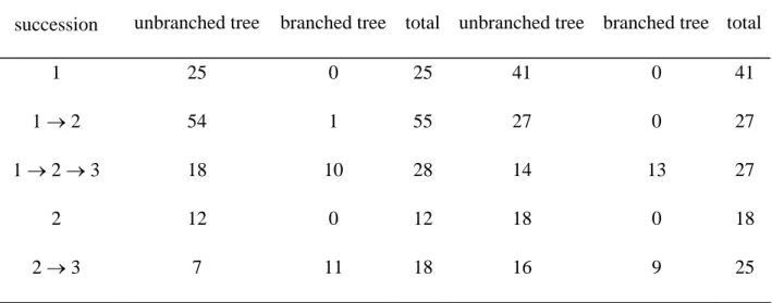
For the “number of leaves” and “annual shoot length” models, all the 22 branched walnuts, except one for the “number of leaves” model, reached growth phase 3 whereas only about 25% of the 116 unbranched walnuts reached this growth phase (25 of 116 for the “number of leaves” model and 30 of 116 for the “annual shoot length” model); see Table 5. For the branched trees, the time interval between the beginning of growth phase 3 and the first branching occurrence was extracted on the basis of the optimal segmentation of the observed sequence computed using the “annual shoot length” model. The mean time interval was 3.33 years (standard deviation: 2.85 years) indicating that the first branching occurrence requires a time interval with respect to the beginning of the third growth phase.

Light environment effect

The growth phase in 2006 (the last year considered), according to the optimal segmentation of the observed sequence computed using the “annual shoot length” model, and the absence/presence of branches, was used to define four tree categories: (i) trees in growth phase 1, (ii) trees in growth phase 2, (iii) unbranched trees in growth phase 3 and (iv) branched trees in growth phase 3. Canopy openness, transmitted light and LMA (during the 2007 growth period) were compared between these four tree categories (Fig. 5). According to the Tukey test, the values computed for the trees in growth phases 1 and 2 were not significantly different for each light environment indicator. These trees had lower values for canopy openness, transmitted light and LMA than trees in growth phase 3. Trees in the first two growth phases were therefore growing in a more shaded environment than trees in growth phase 3. Canopy openness and transmitted light values computed for the unbranched and branched trees in growth phase 3 were not significantly different. LMA was the only indicator with significantly different values between unbranched and branched trees in growth phase 3.

The average tree profile (i.e. ₁+ ₂×

, ,t at

a s

s β

β centered average daily maximum temperature +

1 × 3 ,t a s

β centered cumulative rainfall for each year t) and the predicted tree profile (i.e. average

tree profile value 2 t a t a as s_,ξ , _, τ

+ for each year t) were computed for each tree a on the basis of the

optimal segmentation of the observed sequence and the predicted random effects computed using the “annual shoot length” model. The regression parameters

3 4

1

j

β , β_j2 and β_j3 describe

patterns of change in the mean response over years (and their relationship to explanatory variables) in the walnut population, while

5 6

j a, jξ

τ describes the deviation in growth phase j of

the ath tree profile with reference to the average tree profile; see Fig. 6 for the predicted tree profiles of 6 representative individuals. Four types of tree growth profile were identified:

7 8 9 10 11 12 13 14 15 16 17 18 19 20 21 22 23 24

ƒ Trees characterized by regularly spaced phase changes; see for instance tree 123 where the lengths of growth phases 1 and 2 were similar (4 years in growth phase 1 and 5 years in growth phase 2);

ƒ Trees with constant slow growth; see tree 86 which remained in growth phase 1. These trees remained in unfavorable local conditions (dark understory) throughout the period considered;

ƒ Trees with a long period of slow growth followed by a rapid increase in the annual shoot length corresponding to growth phase changes; see trees 58 and 133. We suspect that these phase changes were due to a rapid modification of the understory light environment enabling a rapid growth increase followed by first branching (see tree 133) despite a long period of slow growth. In this type of tree growth profile, the predicted random effects in growth phases 1 and 3 did not seem to be related and the long phase of slow growth did not seem to affect subsequent tree development;

ƒ Trees with a short period of slow growth before a long period of strong growth; see trees 130 and 124. These trees tended to branch.

1 2 3 4 5 6 7 8 9 10 11 12 13 14 15 16 17 18 19 20 21 22 23 24 25

Tree status with reference to the average tree may be common to all the growth phases but modulated in terms of deviations between growth phases; see for example trees 130 and 124 in Fig. 6. Tree status may also be different in each growth phase; see for example trees 58 and 133 in Fig. 6. The more general assumption of a random effect attached to each growth phase is thus more representative of walnut behavior than the assumption of a random effect common to all growth phases.

Discussion

Walnuts in understory: a shade avoidance response pattern

Trees in the third growth phase in 2006 (the last year considered) were growing in a more luminous environment and had greater LMA than trees in the first two growth phases. Light availability is certainly the main factor that explains a tree's ability to reach the third phase of strongest growth; see Niinemets (1999) for the link between LMA and light availability. Walnuts showed opportunistic growth in understory characterized by their capability to increase their apical growth suddenly in response to a change in the local light environment, for instance arising from a treefall gap. This result is supported by a cross-sectional study of a sub-sample of the same walnut data set (Taugourdeau and Sabatier, 2010). This behavior corresponds to a shade avoidance strategy (Henry and Aarssen, 2001). Because of the sample size (138 trees) and the marked heterogeneity of the studied mixed forest, the local environment of the trees and its time variations can be considered as sufficiently randomized. This explains the emergence of geometric phase length distributions for both the “number of leaves” and the “annual shoot length” models. This contrasts with the successive growth phases with bell-shaped length distributions such as in Corsican pines and sessile oaks in managed forest stands (Chaubert-Pereira et al., 2009). In this latter case, the well-defined successive growth phases

1 2 3 4 5 6 7 8 9 10 11 12 13 14 15 16 17 18 19 20 21 22 23 24 25

were mainly the expression of endogenous equilibriums while in the case studied here, the phase length was the result of an opportunistic process corresponding to a tree's plastic response to environmental changes.

The transition to the third growth phase was related to a reduction in inter-individual heterogeneity. Because of the genetic proximity between the trees (same mother), this may be interpreted as the effect of the local environment on the growth of each tree. In the first two growth phases, young trees, whatever their local environment, were mixed up with older trees in unfavorable local environments while only trees in reasonably favorable local environments reached the third growth phase. This is somewhat similar to the environmental filter concept: see Diaz et al. (1999). A complementary explanation lies in the fact that large trees (in the third growth phase) were less sensitive than smaller trees to the local environment.

Markov switching linear mixed model allowed us to highlight the fact that a long period of suppression has no negative effect on subsequent growth after canopy opening. This is illustrated for instance by tree 58 (Fig. 6) which grew faster than the average tree in the third growth phase despite a long period of suppression corresponding to the first growth phase. Wright et al. (2000) came to the same conclusion on the basis of tree ring data.

Walnut exhibits strong apical dominance in shaded environments since lateral buds only develop after canopy opening (Fig. 7a). This corresponds to a shade avoidance strategy characterized by a major investment in vertical growth to reach higher irradiance strata and a marked response to changes in the light environment (Wright et al., 2000; Henry and Aarssen 2001). This is consistent with the “heliophil status” of walnut. Henry and Aarssen (2001) suggest that a shade tolerance strategy is specific of species growing in the deepest shaded

1 2 3 4 5 6 7 8 9 10 11 12 13 14 15 16 17 18 19 20 21 22 23 24 25

environments and a shade avoidance strategy is specific of species growing in environments characterized by high vertical and horizontal heterogeneity of light availability such as in the studied understory. Light quality was not quantified in this study but is known to be related to the shade avoidance strategy (Franklin and Whitelam, 2005).

Some shade-tolerant species accommodate to a shaded environment by an important lateral development. For instance, fir has long lifespan branches and needles (Mori et al., 2008) in a shaded environment. The response of walnut to shade is very different since it consists of producing juvenile deciduous compound leaves characterized by dentate leaflets.

Effects of temperature and rainfall on annual growth

The effect of average daily maximum temperature and cumulative rainfall was weak in the first phase where shade drastically limited tree development (Fig. 7b). It then increased markedly in the subsequent growth phases. This is consistent both with the results of Mediavilla and Escudero (2004) concerning the response to drought of trees at different stages of development and with the facilitation hypothesis proposed by Holmgren (2000); see also Sack (2004) for a discussion about ecological consequences.

The proposed modeling approach highlighted the positive effect of average daily maximum temperature during shoot organogenesis on the next-year assimilative leaf number (one-year-delayed response). The relationship between temperature and organogenesis has been well established and is the basis of the thermal time concept applied mainly to annual plants (Bonhomme, 2000). The effect of temperature has generally been studied in plants where shoot elongation occurs just after shoot organogenesis, making it difficult to separate the effect on organogenesis from the effect on elongation. In the current study of a temperate perennial

1 2 3 4 5 6 7 8 9 10 11 12 13 14 15 16 17 18 19 20 21 22 23 24 25

species, the one year delay between shoot organogenesis and elongation enabled to clearly decipher the temperature effect. The delay between the change in environment and the plant's response may be an adaptative drawback since such a delayed response may not be appropriate in case of rapid change of the environment (Valladares et al., 2007).

The temperature during organogenesis influences the next-year assimilative leaf number but also, and to a greater extent, the annual shoot length. This result may at first sight appear to be counterintuitive since we did not identify other periods where annual shoot length was affected by average daily maximum temperature. We therefore suspect that the average daily maximum temperature during organogenesis not only influences the number of organs but also the number of cells, and consequently the length of the corresponding internodes; see Ripetti et al. (2008) and references therein.

Modeling forest structure and successional dynamics in a context of climate change

Markov switching linear mixed models were applied to identify and characterize the effects of ontogeny, climatic factors and local environment on tree establishment. At a coarser scale, the outputs of these individual models could be incorporated into models of forest structure and successional dynamics:

ƒ Predictions about possible rank reversal (i.e. changes in interspecific competition) in mixed forest due to climate change can also be made; see Sánchez-Gómez et al. (2008) for a discussion about the ecological consequences of rank reversal. For example, a warmer and drier Mediterranean climate (Christensen et al., 2007) would have antagonist effects on walnut growth: the increased temperature would have a positive effect but the decreased rainfall would have a negative effect. Local rainfall and temperature predictions for 2050 (ARPEGE/IFS model; Déqué et al., 1994) would have

1 2 3 5 6 7 8 9 10 11 12 13 14

a positive effect on the studied walnuts in the third growth phase (+1 leaf and +9 cm per annual shoot) because of the relative importance of temperature on growth. These predictions assume that the selected climatic factors are not subject to threshold effects. ƒ The structure of a population can be characterized at a given date by the proportion of 4

trees in the different growth phases. We expect this classification based on a decomposition of tree growth components to be more robust than alternative classifications based on direct measurements (e.g. diameter measured at breast height).

Acknowledgments

The authors are grateful to Michaël Gueroult for his help in collecting field data, to INRA for freely providing meteorological data, to Yves Caraglio, Pierre Couteron and Nick Rowe for useful comments, to the handling Editor and an anonymous reviewer for their helpful comments that led to an improvement in the presentation of this paper.

Literature cited

Barthélémy D, Caraglio Y. 2007. Plant architecture: a dynamic, multilevel and comprehensive

approach to plant form, structure and ontogeny. Annals of Botany 99: 375-407.

Bonhomme R. 2000. Bases and limits to using ‘degree.day’ units. European Journal of

Agronomy 13: 1-10.

Chaubert-Pereira F, Caraglio Y, Lavergne C, Guédon Y. 2009. Identifying ontogenetic,

environmental and individual components of forest tree growth. Annals of Botany 104: 883-896.

Chaubert-Pereira F, Guédon Y, Lavergne C, Trottier C. 2010. Markov and semi-Markov

switching linear mixed models used to identify forest tree growth components. Biometrics

66(3): 753-762.

Christensen JH, Hewitson B, Busuioc A, Chen A, Gao X, Held I, Jones R, Kolli RK, Kwon W-T, Laprise R, Magaña Rueda V, Mearns L, Menéndez CG, Räisänen J, Rinke A, Sarr

A, Whetton P. 2007. Regional Climate Projections. In: Climate Change 2007: The Physical

Science Basis. Contribution of Working Group I to the Fourth Assessment Report of the Intergovernmental Panel on Climate Change [Solomon S, Qin D, Manning M, Chen Z, Marquis M, Averyt KB, Tignor M, Miller HL. (eds.)]. Cambridge University Press, Cambridge.

Déqué M, Dreveton C, Braun A, Cariolle D. 1994. The ARPEGE/IFS atmosphere model: a

contribution to the French community climate modelling. Climate Dynamics 10: 249-266.

Diaz S, Cabido M, Zak M, Carretero EM, Aranibar J. 1999. Plant functional traits,

ecosystem structure and land-use history along a climatic gradient in central-western Argentina.

Journal of Vegetation Science 10: 651-660.

Dolezal J, Ishii H, Vetrova VP, Sumida A, Hara T. 2004. Tree growth and competition in a

Betula platyphylla-Larix cajanderi post-fire forest in central Kamchatka. Annals of Botany 94:

333-343.

Fitzmaurice GM, Laird NM, Ware JH. 2004. Applied longitudinal analysis. Wiley Series in

Probability and Statistics. Hoboken, NJ: John Wiley & Sons.

Franklin KA, Whitelam GC. 2005. Phytochromes and shade-avoidance responses in plants.

Annals of Botany 96: 169 -175.

Frazer GW, Canham CD, Lertzman KP. 1999. Gap Light Analyzer (GLA), Version 2.0:

Imaging software to extract canopy structure and gap light transmission indices from true-colour fisheye photographs, users manual and program documentation. Simon Fraser University, Burnaby BC, and the Institute of Ecosystem Studies, Millbrook, NY.

Frühwirth-Schnatter S. 2006. Finite Mixture and Markov Switching models. Springer Series

in Statistics. New York: Springer.

Guédon Y, Caraglio Y, Heuret P, Lebarbier E, Meredieu C. 2007. Analyzing growth

Henry HAL, Aarssen LW. 2001. Inter- and intraspecific relationships between shade tolerance and shade avoidance in temperate trees. Oikos 93: 477-487.

Holmgren M. 2000. Combined effects of shade and drought on tulip poplar seedlings: trade-off

in tolerance or facilitation? Oikos 90: 67-78.

Kobe RK, Hogarth LJ. 2007. Evaluation of irradiance metrics with respect to predicting

sapling growth. Canadian Journal of Forest Research 37: 1203-1213.

Kulkarni VG. 1995. Modeling and Analysis of Stochastic Systems. London: Chapman & Hall.

Lacointe A, Kajji A, Daudet FA, Archer P, Frossard JS. 1995. Seasonal-Variation of

Photosynthetic Carbon Flow-Rate into Young Walnut and Its Partitioning among the Plant Organs and Functions. Journal of Plant Physiology 146: 222-230.

Mediavilla S, Escudero A. 2004. Stomatal responses to drought of mature trees and seedlings

of two co-occurring Mediterranean oaks. Forest Ecology and Management 187: 281-294.

Miner B, Sultan S, Morgan S, Padilla D, Relyea R. 2005. Ecological consequences of

phenotypic plasticity. Trends in Ecology & Evolution 20: 685-692.

Mori AS, Mizumachi E, Sprugel DG. 2008. Morphological acclimation to understory

environments in Abies amabilis, a shade- and snow-tolerant conifer species of the Cascade Mountains, Washington, USA. Tree Physiology 28: 815-824.

Niinemets U. 1999. Components of leaf dry mass per area - thickness and density - alter leaf

photosynthetic capacity in reverse directions in woody plants. New Phytologist 144: 35-47.

Pinno BD, Lieffers VJ, Stadt KJ. 2001. Measuring and modelling the crown and light

transmission characteristics of juvenile aspen. Canadian Journal of Forest Research 31: 1930-1939.

Pradal C, Dufour-Kowalski S, Boudon F, Fournier C, Godin C. 2008. OpenAlea: A visual

programming and component-based software platform for plant modeling. Functional Plant

Biology 35(9-10): 751-760.

Ripetti V, Escoute J, Verdeil JL, Costes E. 2008. Shaping the shoot: the relative contribution

of cell number and cell shape to variations in internode length between parent and hybrid apple trees. Journal of Experimental Botany 59: 1399-1407.

Sabatier S, Baradat P, Barthélémy D. 2003a. Intra- and interspecific variations of

polycyclism in young trees of Cedrus atlantica (Endl.) Manetti ex. Carriere and Cedrus libani A. Rich (Pinaceae). Annals of Forest Science 60: 19-29.

Sabatier S, Barthélémy D. 2001. Bud structure in relation to shoot morphology and position

on the vegetative annual shoots of Juglans regia L. (Juglandaceae). Annals of Botany 87(1): 117-123.

Sabatier S, Barthélémy D, Ducousso I. 2003b. Periods of organogenesis in mono- and

Sack L. 2004. Responses of temperate woody seedlings to shade and drought: do trade-offs limit potential niche differentiation? Oikos 107: 110-127.

Sánchez-Gómez D, Zavala MA, Van Schalkwijk DB, Urbieta IR, Valladares F. 2008. Rank

reversals in tree growth along tree size, competition and climatic gradients for four forest canopy dominant species in Central Spain. Annals of Forest Science 65: -.

Segura V, Cilas C, Costes E. 2008. Dissecting apple tree architecture into genetic, ontogenetic

and environmental effects: mixed linear modelling of repeated spatial and temporal measures.

New Phytologist 178: 302-314.

Taugourdeau O, Sabatier S. 2010. Limited plasticity of shoot preformation in response to

light by understorey saplings of common walnut (Juglans regia). AoB PLANTS 2010: plq022, doi:10.1093/aobpla/plq022.

Valladares F, Gianoli E, Gomez JM. 2007. Ecological limits to plant phenotypic plasticity.

New Phytologist 176: 749-763.

Verbeke G, Molenberghs G. 2000. Linear mixed models for longitudinal data. Springer Series

in Statistics. New York: Springer.

Wright EF, Canham CD, Coates KD. 2000. Effects of suppression and release on sapling

growth for 11 tree species of northern, interior British Columbia. Canadian Journal of Forest

Research 30: 1571-1580.

Yagi, T. 2009. Ontogenetic strategy shift in sapling architecture of Fagus crenata in the dense

understorey vegetation of canopy gaps created by selective cutting. Canadian Journal of Forest

Appendix

1

Let

{

}

{

}

(1995) for a general reference about Markov and semi-Markov models. 2 3 4 5 6 Markov chains

A J-state Markov chain

{ }

7

- initial probabilities πj =P

(

)

∑

8

- transition probabilities p_ij = P

(

)

∑

jpij .

9

The implicit occupancy (or sojourn time) distribution of a nonabsorbing state j is the “1-shifted” geometric distribution with parameter

10 jj p − 1 11 12 13 14 15 16 17 18 K , 2 , 1 , ) 1 ( ) (u = −p p −1 u= dj jj ujj

This is the unique discrete memoryless distribution.

Semi-Markov chains

A useful generalization of Markov chains lies in the class of semi-Markov chains, in which the process moves out of a given state according to an embedded Markov chain with self-transition

probability in nonabsorbing states ~ =p_jj 0 and where the time spent in a given nonabsorbing

state is modeled by an explicit occupancy distribution. 19

20 21

22 A J-state semi-Markov chain

{

}

- initial probabilities π_j =P

(

)

∑

jπj ;

- transition probabilities 1

ƒ nonabsorbing state i: for each j ≠i,p~_ij =P

(

)

1

2

~ =

∑

p

3

ƒ absorbing state i: p_ii =P

(

)

4 5

6 An explicit occupancy distribution is attached to each nonabsorbing state:

( ) (

)

d_{j t u t u v t t}

7

8 Since t=1 is assumed to correspond to a state entering, the following relation is verified

(

)

We define as possible parametric state occupancy distributions negative binomial distributions

with an additional shift parameter d ( ) which defines the minimum sojourn time in a given

state. The negative binomial distribution with parameters d, r and p, NB(d, r, p), where r is a

real number ( ) and , is defined by

1 ≥ d 0 > r 0< p≤1

( )

A Markov chain can be reparameterized as a semi-Markov chain such that for each

nonabsorbing state i, ~p_ij = p_ij/

(

)

occupancy distribution is the “1-shifted” geometric distribution NB(1, 1, .

18 19 20 ii p − 1 )

Hidden Markov chains

1 2

}

3 A hidden Markov chain can be viewed as a pair of stochastic processes

{

“output” process

{

t t Y S ,

}

Y

{ }

by a probabilistic function or mapping denoted by f (hence 4

)

( _t

t f S

Y = ). Since the mapping f is

such that a given output may be observed in different states, the state process

{

observable directly but only indirectly through the output process 5

6 St

}

{ }

is related to the Markov chain 7

{ }

{ }

= 1

by the observation (or emission) probabilities

with in the case of a continuous output process. The

definition of observation probabilities expresses the assumption that the output process at time t depends only on the underlying Markov chain at time t.

8 9 10 11 12 13 14 15

(

)

∫

Markov switching linear mixed models

Let be the observed variable and let be the non-observable state for individual a

( ), at time t ( ). The output process

t a Y , , 1_K = t a S , N

a , t =1,K,Ta

{ }

mixed model for individual a is related to the state process 16

{ }

chain, by a linear mixed model (a linear mixed model can be viewed as an extension of a classical linear model where random effects are added to fixed effects); see Verbeke and Molenberghs (2000). It assumes that the vector of repeated measurements for each individual follows, in each state, a linear regression model where some of the regression parameters are population-specific (i.e. the same for all individuals), whereas other parameters are individual-specific. In our case, the individual status (compared with the average individual) is assumed to be different in each state:

17 18 19 20 21 22 23 24

). , 0 ( N ~ | ), 1 , 0 ( N ~ , , state Given 2 , , , , , , , , , , , , , , , t a t a t a t a t a s t a t a t a s a t a s a s s t a t a t a t a s S X Y s S σ ε ξ ε ξ τ β = + + = = 1

2 The Gaussian observation probabilities are defined as follows:

(

)

4 In this definition, is the Q-dimensional row vector of explanatory variables for individual

a at time t. Given the state ,

t a X , t a t a s S _, = _, t a s _,

β is the Q-dimensional fixed effect parameter vector, 5

t a s a, _,

ξ is the individual a random effect,

t a s _,

τ is the standard deviation for the random effect and is the residual variance. The individuals are assumed to be independent. For convenience, random effects are assumed to follow the standard Gaussian distribution. The random effects for an individual a are assumed to be mutually independent (

6 7 8 2 ,t a s σ j i j a i a , )= ;0 ≠ cov(ξ _, ξ _, ).

Observations in different states for an individual a are assumed to be conditionally independent

given states (for , if and

if 9 10 11 t≠t' 2 ,t a s sa,t 0 ) | , _{,' ,1 ,1} , = = a a T a T a t a t a Y S s Y cov( ' ,t a s ' , ,t at a s s ≠ 1 , a T a s = 1 , ' , ,, | ) a T a t a t a Y S =τ

cov(Y = where denotes the

-dimensional vector of non-observable states for individual a).

) ,T_a a S Ta , , , ( ,1 ,2 1 , a a a T a S S S = _K 12 13 14 15 16 17 18 19 20

Semi-Markov switching linear mixed models

In the same manner as for a Markov switching linear mixed model, a semi-Markov switching linear mixed model can be defined, the only difference being the replacement of the underlying Markov chain by an underlying semi-Markov chain.

state 1 state 2 log-likelihood SMS-LM NB(1, 1.56, 0.16) NB(1, 1.17, 0.11) -2241.86 9.2, 7.15 10.27, 9.09 MS-LM NB(1, 1, 0.1) NB(1, 1, 0.09), -2242.7 No. leaves 9.62, 9.1 11, 10.47 SMS-LM NB(1, 1.91, 0.13) NB(1, 1.3, 0.16) -3913.06 13.63, 9.81 7.83, 6.54 MS-LM NB(1, 1, 0.07) NB(1, 1, 0.12) -3915.95 Annual shoot length 15.19, 14.67 8.19, 7.67

Table 1. “Number of leaves” and “annual shoot length” models: Estimated occupancy distributions (parameters, mean and standard deviation in years) for states 1 and 2 for the three-state semi-Markov switching linear model (SMS-LM) and Markov switching linear model (MS-LM).

1 11,λ

p p₂₂,λ₂ η₃

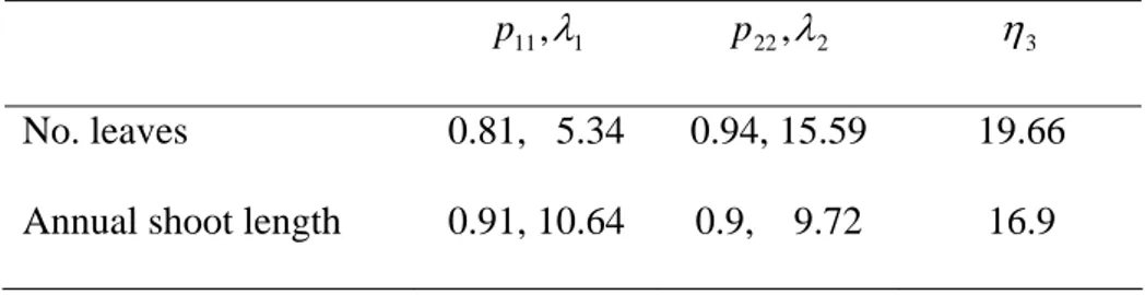
No. leaves 0.81, 5.34 0.94, 15.59 19.66

Annual shoot length 0.91, 10.64 0.9, 9.72 16.9

Table 2. Markov switching linear mixed models: self-transition probabilities and

corresponding mean time

ii p

i

λ spent in the transient states 1 and 2 (in years), and mean time up to

the first occurrence of state 3 η3 (in years) for the “number of leaves” and the “annual shoot

length” models. It should be noted that η3 <λ1+λ2 since a certain proportion of the trees

started directly in state 2 (with π₂ =0.21 for the “number of leaves” model andπ₂ =0.32 for

state 1 2 3 intercept β_j1 (s.e.) 3.36 (0.03) 4.47 (0.04) 6.21 (0.12) temperature parameterβ_j2 (°C-1) (s.e.) 0.08 (0.02) 0.17 (0.03) 0.48 (0.09) regression parameters

average temperature effect ) ( mad 2 2 j X j × β _{0.09 0.15 0.38} random variance τ2j (s.e.) 0.41 (0.45) 0.52 (0.39) 0.29 (0.61) residual variance σ2_j (s.e.) 0.23 (0.01) 0.57 (0.02) 0.7 (0.05) total variance Γj2 0.64 1.09 0.99 variability decomposition proportion of inter-individual heterogeneity 65.08% 47.71% 29.29% marginal observation distribution (μ_j,Γ_j) _{3.36, 0.8 4.56, 1.04 6.55, 0.99}

Table 3. Number of leaves per annual shoot: Estimated Markov switching linear mixed model parameters and marginal observation distributions for each state. For each observation linear mixed model the intercept, the regression parameter for the average daily maximum temperature, the average daily maximum temperature effect and the variability decomposition are given. Standard errors are given in parentheses.

state 1 2 3 intercept β_j1 (cm) (s.e.) 4.01 (0.06) 5.86 (0.14) 12.11 (0.74) temperature parameter β_j2 (cm °C-1) (s.e.) 0.13 (0.05) 1.53 (0.11) 4.25 (0.6) average temperature effect

) ( mad ₂ 2 j X j × β (cm) _{0.15 1.68 2.61} cumulative rainfall parameter β_j3 (cm mm-1) (s.e.) 0.5 10-3 (0.2 10-3) 4. 10-3 (0.4 10-3) 5. 10-3 (1.4 10-3) regression parameters

average cumulative rainfall effect ) ( mad ₃ 3 j X j × β (cm) _{0.08 0.54 0.72} random variance τ2_j (s.e.) 0.99 (0.51) 3.82 (0.63) 9.96 (1.71) residual variance σ2j (s.e.) 1.3 (0.01) 4.7 (0.21) 29.01 (2.04) total variance Γ2_{j 2.29 8.52 38.97} variability decomposition proportion of inter-individual heterogeneity 43.23% 44.84% 25.56% marginal observation distribution (μj,Γj) (cm) 4.01, 1.51 6.73, 2.92 15.28, 6.24

Table 4. Annual shoot length: Estimated Markov switching linear mixed model parameters and marginal observation distributions for each state. For each observation linear mixed model the intercept, the regression parameter for the average daily maximum temperature, the average daily maximum temperature effect, the regression parameter for cumulative rainfall, the cumulative rainfall effect and the variability decomposition are given. Standard errors are given in parentheses.

number of leaves per annual shoot model annual shoot length model

profile of state

succession unbranched tree branched tree total unbranched tree branched tree total

1 25 0 25 41 0 41

1 → 2 54 1 55 27 0 27

1 → 2 → 3 18 10 28 14 13 27

2 12 0 12 18 0 18

2 → 3 7 11 18 16 9 25

Table 5. Number of trees with the same profile of state succession extracted from the optimal segmentations computed using the estimated Markov switching linear mixed models. A profile of state succession is defined as the series of distinct states visited along the sequence regardless the time spent in each state.

(c) 12 to 16 years old 0 5 10 15 20 25 30 35 40 45 50 1977 1979 1981 1983 1985 1987 1989 1991 1993 1995 1997 1999 2001 2003 2005 Year S h oot l engt h (c m )

(a) < 8 years old

0 5 10 15 20 25 30 35 40 45 50 1997 1998 1999 2000 2001 2002 2003 2004 2005 2006 Year S h oot l engt h (c m ) (d) > 16 years old 0 5 10 15 20 25 30 35 40 45 50 1977 1979 1981 1983 1985 1987 1989 1991 1993 1995 1997 1999 2001 2003 2005 Year S h o o t l e n g th ( c m ) (b) 8 to 11 years old 0 5 10 15 20 25 30 35 40 45 50 1997 1998 1999 2000 2001 2002 2003 2004 2005 2006 Year S h oo t l eng th (c m )

Figure 1. Length of successive annual shoots along walnut main stems (a) less than 8 years old, (b) from 8 to 11 years old, (c) from 12 to 16 years old, (d) more than 16 years old. The very first annual shoot corresponding to the germination year is not shown.