Very low field magnetic resonance imaging

HAL Id: tel-01064053

https://tel.archives-ouvertes.fr/tel-01064053

HAL is a multi-disciplinary open access

archive for the deposit and dissemination of sci-entific research documents, whether they are pub-lished or not. The documents may come from teaching and research institutions in France or abroad, or from public or private research centers.

L’archive ouverte pluridisciplinaire HAL, est destinée au dépôt et à la diffusion de documents scientifiques de niveau recherche, publiés ou non, émanant des établissements d’enseignement et de recherche français ou étrangers, des laboratoires publics ou privés.

Very low field magnetic resonance imaging

Quentin Herreros

To cite this version:

Quentin Herreros. Very low field magnetic resonance imaging. Other [cond-mat.other]. Université René Descartes - Paris V, 2013. English. �NNT : 2013PA05T056�. �tel-01064053�

V E R Y L O W F I E L D M A G N E T I C R E S O N A N C E I M A G I N G

Cette thèse, préparée au laboratoire SPEC (CEA\DSM\IRAMIS) au sein du groupe NanoMagnétisme et Oxydes, a été encadrée par

C O N T E N T S

1 m a g n e t i c r e s o na n c e i m a g i n g : principle 9

1.1 Nuclear Magnetic Resonance . . . 10

1.1.1 Polarization and Nuclear Spin . . . 10

1.1.2 Excitation and Nuclear Resonance . . . 11

1.1.3 Basic Sequences . . . 14

1.1.4 Magnitude of low field NMR signal . . . 15

1.1.5 Polarization Enhancement . . . 17

1.1.6 Signal-to-noise ratio . . . 19

1.1.7 Sample Noise . . . 20

1.2 Spatial encoding and imaging features at very low field 22 1.2.1 Frequency encoding and K-space definition . . 22

1.2.2 Phase Encoding . . . 24

1.2.3 Slice Selection . . . 24

1.2.4 Resolution . . . 26

1.2.5 Field Of View . . . 27

1.2.6 Signal to Noise Ratio . . . 27

1.2.7 Contrast-to-noise ratio . . . 28

2 e x p e r i m e n ta l s e t u p 32 2.1 Permanent field and homogeneity . . . 33

2.1.1 Different kind of magnets . . . 33

2.1.2 Homogeneity required . . . 34

2.1.3 Coils design . . . 35

2.1.4 Small size setup . . . 36

2.1.5 Full size setup . . . 38

2.1.6 Measurements of strength and homogeneity . . 41

2.2 Gradients and RF pulses . . . 44

2.2.1 Gradient specificity . . . 44

2.2.2 Gradient strength and linearity required . . . . 44

2.2.3 Small size setup . . . 45

2.2.4 Full size setup . . . 47

2.2.5 Strength and linearity measurement . . . 49

2.2.6 RF coil . . . 52

2.3 RMN Spectrometer . . . 55

2.3.1 Emission part . . . 55

2.3.2 Reception part . . . 55

2.3.3 Shims and Gradients . . . 57

3 f e m t o t e s l a s e n s o r s 59 3.1 Tuned coils . . . 60

3.1.1 RLC Circuit . . . 60

3.1.2 Detectivity . . . 62

3.1.3 Pulses and noise . . . 64

3.1.4 Nuclear Magnetic Resonance . . . 65

3.2.2 SQUIDs for MRI . . . 69

3.2.3 Atomic Optical Magnometers . . . 71

3.2.4 Atomic Optical Magnetometers for MRI . . . . 73

3.3 Mixed sensors : Theory . . . 75

3.3.1 Giant MagnetoResistive Sensor . . . 75

3.3.2 Superconducting Flux-To-Field Transformer . . 78

3.3.3 Superconductive loop Inductance . . . 79

3.3.4 Noise sources . . . 80

4 m i x e d s e n s o r s f o r v e r y l o w f i e l d m r i 83 4.1 Characterization of mixed sensors . . . 84

4.1.1 GMR Characterization . . . 84

4.1.2 Bridge Configuration . . . 85

4.1.3 Mixed sensor Characterization . . . 87

4.1.4 Preamplifier . . . 89

4.1.5 Detectivity . . . 90

4.1.6 Very Low Field MRI applications . . . 92

4.2 Introduction to flux transformers . . . 96

4.2.1 Non resistive flux transformer . . . 96

4.2.2 Resistive flux transformer . . . 99

4.2.3 Tuned flux transformer in series . . . 101

4.3 Implementation of flux transformers . . . 103

4.3.1 Resistance . . . 103

4.3.2 Coupling . . . 104

4.3.3 Size of the sensor . . . 107

4.3.4 Noise, signal and MRI devices . . . 108

4.3.5 Nuclear Magnetic Resonance . . . 109

5 c l a s s i c s e q u e n c e s 112 5.1 First steps into imaging . . . 113

5.1.1 Double phase encoding . . . 113

5.1.2 Slice selection . . . 115

5.1.3 Mixed sensors vs tuned coils . . . 116

5.1.4 Susceptibility artifacts and metallic implants . . 118

5.1.5 In-vivo imaging . . . 121

5.2 Relaxometry . . . 122

5.2.1 Definition . . . 122

5.2.2 Multi spin echo sequence . . . 123

5.2.3 Inversion Recovery sequence . . . 125

5.2.4 Liquid relaxometry . . . 127

5.2.5 In-vivo relaxometry . . . 128

6 s p e e d i n g u p a c q u i s i t i o n t i m e 132 6.1 FLASH for very low field MRI . . . 133

6.1.1 Definition . . . 133

6.1.2 Very low field specificity . . . 134

6.2 Spiral acquisition . . . 140

6.2.1 Principle . . . 140

6.2.2 Very low field specificity . . . 141

6.2.3 EPI for 2 dimensional imaging . . . 144

Nuclear Magnetic Resonance (NMR) is a physical phenomenon en-abling the observation of quantum mechanical properties of specific atomic nucleus. It has been extensively developed to study physi-cal, chemical and biological properties of matter through NMR spec-troscopy. It occurs when the nuclei of specific atoms are immersed in an external magnetic field B0 perfectly homogeneous. This mag-netic field is expressed either in Tesla or in Oersted (1 Oe = 0.1 mT). Usually, it needs to be of high intensity which means tens of thou-sand times stronger than the natural earth’s magnetic field. Typically a clinical MRI works between 1.5 T and 3 T and the earth’s magnetic field has been measured between 0.250 Oe and 0.65 Oe [11]. Another use of the nuclear property has been proposed with Magnetic Reso-nance Imaging (MRI). This widely used medical imaging technique offers relevant clinical diagnosis with a precise spatial representation of specific biological properties. However this method presents some serious drawbacks due to the use of this large magnetic field. To gen-erate such homogeneous field at this strength, superconducting coils are used. These constituents are costly to purchase and to maintain which turns MRI into an expensive imaging protocol. The homogene-ity requirements impose a confined design which raises important difficulty for claustrophobic patient (5-7% of the population) [2]. The

c o n t e n t s 6

comfort of the device is also degraded by gradient generating impor-tant acoustic noises. Finally, the use of high field excludes de facto any MRI on patient with pacemakers, earth valves, metallic implants on brain, eyes or ears and infusion catheters because of heating, small displacements and artifacts. Despite those issues, High Field MRI has been extensively developed for clinical uses as the NMR signal am-plitude is proportional to the magnetic field strength. Thus the per-formance of MRI experiments scales as the magnetic field intensity. Moreover, Radio-Frequency (RF) tuned coils are used to measure sig-nals at those fields and their detectivity scales also as the magnetic field intensity. All put together, the efficiency of the MRI setup in-creases roughly as the square of the field. This explains the develop-ment of very high field MRI up to 11.7 T [55].

Another approach has been proposed in Very Low Field MRI and Ultra Low Field MRI with the conception of new kind of sensors much more efficient than RF coils for low frequencies. Those configu-rations can rely on inexpensive resistive coils for the permanent field with an open and light design. Free of any acoustic noises, this tech-nique reduces all safety issues induced by high magnetic fields. Su-perconducting Quantum Interference Devices (SQUIDs) and Atomic Magnetometers are well known sensors presenting a good detectiv-ity competitive with RF coils at low and ultra low field. Through the work of J. Clarke et al. [13], the use of SQUIDs for ultra low field MRI has been proven. Imaging was performed at 132 µT with a pre-polarizing field between 40 and 60 mT. The signal was acquired with a SQUID working at 4 Kelvin and combined with an untuned flux transformer. I. Savukov et al. [50] demonstrated the use of Atomic Magnetometer for in vivo imaging at 2 mT with a pre-polarizing field at 200 mT through a tuned flux transformer. Moreover a recent study led by S. Busch et al. [10] has proven that new relaxation mechanisms at low field could lead to new opportunities for clinical diagnosis. Very and Ultra Low Field MRI appear like promising complementary methods to classical clinical MRI.

In 2004, C. Fermon and M. Pannetier-Lecoeur proposed a new kind of sensor called “Mixed Sensors” [45]. Combining a Giant Magne-toresistance (GMR) with a superconducting loop, it delivers a flat response in frequency and may compete with SQUIDs in term of de-tectivity at very low field. Depending on the superconducting loop material used, its working temperature can be at 4 Kelvin ( Low TC Niobium) or 77 Kelvin ( High TCYBa2Cu3O7−d). The structure of the sensor makes him resistant against external magnetic perturbation which is essential for any use in MRI conditions.

The goal of this study is to integrate High TC mixed sensors into two Very Low Field MRI setups. Working with a static field from 1 mT to 10 mT, MRI experiments are performed to evaluate the possibility offered by such system in comparison to existing tools.

High TC mixed sensors are characterized precisely outside and in-side an MRI environment, with pulses and gradients, to test their robustness in working conditions. A comparison between their detec-tivity and other existing sensors (tuned coils, atomic magnetometer and SQUIDs) is performed, at different frequencies. Finally, the use of different kind of flux transformers is discussed analytically and ex-perimentally. They are broadly used with SQUIDs and Atomic Mag-netometer and an optimal configuration adapted to this particular sensor is proposed.

To obtain a clean MRI image, strict conditions must be respected leading to complex coil architectures. Two Very Low Field MRI setups are used : one existing system adapted for small sample (working vol-ume of 5*5*5 cm3) and one new full-head system adapted for in-vivo brain imaging (working volume of 15*15*15 cm3). Adjusted to gener-ate a field between 1mT and 10 mT, both are using no pre-polarization field at all. The absence of any pre-polarizing step offers more free-dom in sequence optimization and also less perturbations induced by eddy currents. For practical use and comfort of utilization, open de-sign is favored and no dedicated shielded room is used. Permanent field, gradients and RF pulses are precisely characterized and opti-mized to fit specific requirements at such field. A special attention is paid to homogeneity, amplitude and slew rates as those parameters are critical to build an operative MRI.

A homemade spectrometer and an MRI software are engineered to control both setups with maximum flexibility. Classic spin echo and gradient echo sequences are tested for first imaging tests. Three dimensional images are acquired at different field strength with spe-cific phantoms used to test the robustness of the system and iden-tify problematic artifacts. Indeed the NMR signal is a very precise tool to estimate characteristics of an external magnetic field. Then contrasts are enhanced by using adapted sequence (Echo time, Rep-etition time,...). The determination of accurate values has required a relaxometry study of tissues and liquids of interests.

Finally, over the past fifty years, high field MRI has seen its acqui-sition time decreased by a factor thousand. This gigantic reduction of the time needed to image human tissues has been possible with the use of specific sequences called “fast sequences”. Many different methods have been developed but all of them try to reduce the

ac-c o n t e n t s 8

quisition time to the minimum required to measure a signal. The use of those techniques are discussed for very low field MRI through the use of two well known sequences : Fast Low Angle SHot sequence (FLASH) and Echo Planar Imaging (EPI). Their relevancy at very low field is analyzed through analytical and experimental measurements.

1

First MRI scan of a live human being chest performed in 1977 [17]

ased on the discovery of Nuclear Magnetic Resonance spectroscopy by Bloch and Purcell in 1945, Magnetic Resonance Imag-ing has become a major medical imagImag-ing technique. In this chapter, I will introduce some general notions about nuclear resonance. Ori-gins and manipulations of the nuclear magnetic moment will be de-veloped. I will also present several specific aspects of very low field NMR. Then an introduction to MRI will present basics of imaging techniques. Through the study of MRI properties, strong and weak points of very low field MRI will be enlightened.

1.1 nuclear magnetic resonance 10

1.1 n u c l e a r m a g n e t i c r e s o na n c e

Nuclear Magnetic Resonance has been extensively developed for med-ical application through Magnetic Resonance Imaging. Usually, those devices are working with high permanent field. The use of very low permanent field induce new properties. In this section, the polariza-tion and the resonance of the nuclear magnetic moment are intro-duced. Its frequency and its amplitude for very low field MRI is pre-dicted analytically. The combination of pulses to measure the NMR signal is explained through the presentation of basic sequences. The signal-to-noise ratio problematic in MRI experiments is presented as well as different methods to enhance the nuclear polarization of sam-ples. Finally, the magnetic noise generated by the body is briefly dis-cussed from very low field perspective.

1.1.1 Polarization and Nuclear Spin

As points it out the name, Nuclear Magnetic Resonance is a physical phenomenon related to atoms nuclei. Those nuclei are composed of neutrons and protons which both have the intrinsic quantum prop-erty of spin. In classical physics, a spin can be seen as the rotation of the charge around its own axe. This spin, or angular momentum,~I is quantified and induces a magnetic moment~µsuch as :

~µ= ¯hγ~I

where ¯h is the reduced Planck constant and γ the gyromagnetic ratio of the particle. The overall magnetic moment of a nucleus is then related to a magnetic moment M~0 = ∑~µ. This magnetic moment is a critical parameter for NMR measurement. However an even mass nucleus with an even number of neutrons present a zero overall spin (_∑~I = 0) which is not interesting from the NMR point of view. For others nuclei (∑~I ≥ 1

2) in absence of external interactions, all spin states are degenerated which lead to M~0 = 0. The application of an external magnetic field B0will break degeneracy and spin states will no longer have the same energy.

Figure 1.1: Spin states and magnetic field

For most MRI applications, the nucleus1_{H is used as it is present in} H2O, a dominant component in the human body . Figure1.1presents this behavior for nucleus with a spin of one-half ( like 1H ). This difference in energy results in a small population bias toward the lower energy state and the apparition of an overall magnetic moment

~ M0. For1H, we have : M0= Nγ2¯h2B0 4kbT (1.1) where N is the spin density, k_b is the Boltzmann constant and T the temperature. This magnetic moment has the same direction as B0. The use of a magnetic field to generate a magnetization inside a sample is called the polarization.

Field7(B

)

Figure 1.2: Field (B0) and frequency range of MRI

In this thesis, we are typically working between 1 mT and 10 mT, in the very low field MRI range.

1.1.2 Excitation and Nuclear Resonance

The measurement of this magnetic moment is impossible as it is merged into the external magnetic field which is much larger. How-ever, a tip down of the magnetic moment can be achieved with the use

1.1 nuclear magnetic resonance 12

of a radio-frequency pulse. An electromagnetic excitation is applied on the sample at the Larmor Frequency

v0 = γ 2πB0

This will result in a magnetic resonance absorption and an increase of the high energy state population. At the end of the pulse, the mag-netic moment will relax to its original equilibrium state with an an-gular speed ω0=2πv0.

Nucleus Gyromagnetic factor γ/2π (MHz/T) v0at 3T (Mhz) v0at 10 mT (kHz) 1_H 42.58 127 426 13_C 10.69 32.1 107 15_{N 4.31 12.9 43.1} 31_{P 17.21 51.6 172}

Table 1.1: Commonly observed nuclei (∑~_{I = 1/2) and their resonance}

fre-quency at 3 T and 10 mT

This relaxation is well described by Bloch equations. For transverse components, we have

dMx,y(t)

dt =γ( ~M(t) × ~B(t))x,y−

Mx,y(t) T2

where T2 is the spin-spin relaxation time. It is inversely proportional to the intrinsic inhomogeneity of the sample. For the longitudinal component, we have

dMz(t)

dt =γ( ~M(t) × ~B(t))z−

Mz(t) −M0 T1 where T1is the spin-lattice relaxation time.

X Y Z RF Pulse

Excitation

Relaxation

Polarization

Figure 1.3: Nuclear Magnetic Resonance of a water bottle for a π

2 pulse. The

magnetic moment M is described at different stage.~

The detection always needs to be orthogonal to the polarization field B0 to measure the transverse components of the magnetic mo-ment. Thus, in perfect homogeneity conditions, T2 can be measured

straightly with the Free Induction Decay (FID). According to setup requirements and sensors robustness, the detection can be either in the same direction of the pulse or perpendicular to it ( for quadrature-phase acquisition). The use of a Fourier Transform allows to convert this temporal signal into its frequency distributed equivalent. It is useful for measuring its amplitude and its bandwidth but especially for imaging purpose as we will see in the next section. It has to be no-ticed that the Fourier Transform is applied using a specific algorithm called “Fast Fourier Transform”. This method reduces dramatically the number of operations needed but requires a cartesian distribu-tion of acquisidistribu-tion points.

-1.5 -1 -0.5 0 0.5 1 1.5 0 20 40 60 80 100 120 140 Amplitude (V) Time (s) (a) 0 0.02 0.04 0.06 0.08 0.1 0.12 0.14 0.16 0.18 0.2 -4000 -3000 -2000 -1000 0 1000 2000 3000 4000 Amplitude (V) Frequency (Hz) (b)

Figure 1.4: a) Free Induction Decay of a Nuclear Magnetic Resonance signal and b) its Fast Fourier Transform

The NMR signal is oscillating at the Larmor Frequency, which im-plies that it depends on the applied field B0and on the gyromagnetic factor γ of the nucleus (see Table1.1). An inhomogeneous permanent field B0+δB will result in a bandwidth widening of the NMR sig-nal ( v0+δv ) and a faster decoherence between spin phases. Thus it leads to a weakening of signal amplitude and a shorter measured T2( called T2∗). Coils that generate B0need a specific design to maximize homogeneity to reach the intrinsic spin-spin relaxation of the sample. The higher the field is, the harder it becomes to have a good homo-geneity. We will see in this Chapter 2.1 that Very Low Field MRI is not disadvantaged by this particular constrain.

1.1 nuclear magnetic resonance 14

1.1.3 Basic Sequences

A sequence can be define as a specific pattern of pulses and gradients (see Chapter 1.2) to measure Nuclear Magnetic Resonance. Complex sequences will be studied in Chapter 6. We will present here just basic sequences, that will be used for a better understanding of future developments.

Free Induction Decay sequence is the use of a single RF pulse to tip the magnetic moment of an angle α. Usually α = π

2 to maximize the amplitude of detected signals.

RF Signal

Figure 1.5: Free Induction Decay Sequence

Spin Echo sequence is the use of one excitation pulse α followed by a refocusing pulse π . This sequence is used to get rid of phase decoherence due to external inhomogeneity. Let’s take two spins a and b at t=0 in phase (∆ϕ= ϕa,0−ϕb,0=0 ) . Inhomogeneous field Bp(x, t)and intrinsic inhomogeneity of the sample Bi(x, t)introduce a decoherence over time such as

 



ϕa,t = ϕa,0+ϕ_Bp(a,t)+ϕBi(a,t)

ϕb,t = ϕb,0+ϕ_Bp(b,t)+ϕBi(b,t)

and then

∆ϕ= ϕ_Bp(a,t)+ϕ_Bi(a,t)−ϕ_Bp(b,t)−ϕ_Bi(b,t)

A π pulse inverse the phase and we obtain ϕx,t = −ϕx,t. After a time t0, we will obtain

 



ϕa,t+t0 = −_ϕa,0−_ϕBp(a,t)−_ϕB

i(a,t)+ϕBp(a,t0)+ϕBi(a,t0) ϕb,t+t0 = −_ϕb,0−_ϕBp(b,t)−_ϕBi(b,t)+_ϕBp(b,t0₎+ϕ_Bi(b,t0₎

and then

∆ϕ= −ϕ_Bp(a,t)+ϕBp(a,t0₎−ϕ_Bi(a,t)+ϕBi(a,t0)+. . . . . . ϕ_Bp(b,t)−ϕBp(b,t0₎+ϕ_Bi(b,t)−ϕBi(b,t0₎

The intrinsic inhomogeneity is random and then it is not symmetrical with the refocusing pulse. However an external perturbation Bp(x, t)

can be symmetrical (if it is constant for exemple). That way, the de-phasing becomes

∆ϕ= −ϕ_Bi(a,t)+ϕBi(a,t0)+ϕBi(b,t)−ϕBi(b,t0)

Only the decoherence of the intrinsic inhomogeneity remains. Thus Spin Echo can be used to access the “real” T2 in inhomogeneous en-vironment. It is also relevant for three dimensional imaging and the use of frequency coding (see Chapter 1.2).

RF Signal

Echo Time (TE)

Figure 1.6: Spin Echo Sequence

Regardless the method, the separation time between two sequences is an important parameter (see Chapter 1.2) which is called the rep-etition time (TR). In a Spin Echo, the separation time between the excitation pulse and the refocusing pulse is called the Echo Time (TE). 1.1.4 Magnitude of low field NMR signal

It is of prime importance to have an idea of the signal strength of a sample. It defines the minimum required detectivity of a sensor to measure the signal without any averaging. We define a sample as a cube of water of 1 cm3. We consider this sample just after a theoretical pulse of π

2. Thus this cube can be decomposed in magnetic dipoles of 1mm3 with a magnetic moment~m.

1.1 nuclear magnetic resonance 16

Figure 1.7: Description of the sample In this configuration, the dipole equation is

~ B= µ0 4πr3(3 ~ m.~r r2 .~r− ~m)

where µ0is the vacuum permeability and~B is the magnetic field gen-erated by the moment ~m at the position~r(x, y, z). Magnetic sensors are just measuring one component of the field which correspond to Bzsuch as Bz = mµ0 4πr3(3 z2 r2 −1)

The magnetic moment m of 1 elementary dipole can be estimated using3.1. The number of proton H inside 1 mm3 is :

N =2NA M_1mm3

MH2O

=6.7∗1019

Then, at 300K, under a permanent field of 10 mT, we have m=3.3∗10−14 A.m2

The contribution of all magnetic dipole are added up to obtain the generated magnetic field profile (Figure1.8).

Figure 1.8: Field magnitude generated by a water sample (in white) At a distance of 1 cm, the field amplitude along z is around 1 pT. In a low noise environment, it gives an order of magnitude of the minimum required detectivity to see the signal with one acquisition at 10 mT. It has to be compared with the same sample in a classical high field MRI at 3 Tesla. At 1 cm, the field magnitude along z is 300 times stronger (300 pT). Using a high magnetic field provide a better signal and then a better quality image. New MRI devices have been built to perform clinical study at 7T [37].Very Low Field MRI presents a clear disadvantage in terms of signal.

1.1.5 Polarization Enhancement

This limitation in polarization is intimately linked to very low field study. However, some solutions exist to overcome this restriction.

Magnetization pre-polarization is a field cycling method. A high magnetic field is applied during a time T1 on the sample to get a large polarization. Then the spin precession is measured in the low permanent field. In this way the signal is strongly enhanced. The pre-polarization field doesn’t need to be homogeneous as it is ap-plied before acquisition time. This allow the use of simple and cheap coil designs. However it presents some drawbacks. First, the pre-polarization phase is time consuming and needs to be repeated after each pulse which is a strong constrains on the used sequences. Sec-ondly, this method still excludes all metallic implants. Finally, low field MRI usually needs shielded environment which are subject to strong Eddy currents induced by strong field variations. Those un-desired currents perturb the overall homogeneity. This method has

1.1 nuclear magnetic resonance 18

been used with SQUIDs for in vivo Ultra Low Field MRI [41] and for microfluidic applications [56].

Hyperpolarization of noble gasesis frequently used to image porous media such as lungs [42]. Atoms like129Xe and 3He (nuclear spin of 1/2) can see their magnetic moment enhanced by interaction with a pumped atomic alkali vapor like rubidium (Rb). Electrons of an alkali metal vapor are polarized with a laser beam and then this po-larized electronic state is transferred to the noble gas through a spin-exchange interaction.

Figure 1.9: Hyperpolarization steps for129Xe

The nuclear polarization of the noble gas can be up to 10%. In comparison, the1H polarization at 10 mT is around 0.02 ppm.

Dynamic Nuclear Polarization, based on Overhauser effect [44], enhances the nuclear magnetization by transferring spin polarization from electrons to nuclei. Free radicals (unpaired electron spins) are usually added to the studied sample. A Radio-Frequency irradiation of the two-spin system at the frequency of the electron spin reso-nance (ESR) is applied.When the saturation is reached, a transfer of polarization from electron to nuclear spin starts. The non-equilibrium polarization created is much larger than the corresponding thermal equilibrium polarization. One promising use of DNP for in vivo imag-ing is called DNP hyperpolarization or DNP dissolution [6]. The idea is to perform DNP on a solid state sample under 3 T at a tempera-ture around 1K. The polarization is increased by a factor 10000 and is preserved when the solid is dissolved in a liquid phase. This hy-perpolarized liquid is then separated from free radicals and injected in vivo. However this method is limited to nuclear spins with a long longitudinal relaxation time T1(like13C and15N ).

Those methods are not used here in this thesis but could be imple-mented to the existing setup for future research.

1.1.6 Signal-to-noise ratio

Those efforts to increase the polarization fit into the overall project of increasing signal-to-noise ratio (SNR). Magnetic Resonance Imaging depends strongly on this parameter as it is directly involved in the quality of the image. It can be defined as the power ratio between the meaningful information P_signal and the background noise Pnoise.

SNR= Psignal

Pnoise

Figure 1.10: Signal-to-noise ratio for a nuclear magnetic resonance signal Some other solutions than doping polarization are briefly presented here to maximize it :

• One option concerns the detection chain. An efficient sensor presents a low intrinsic noise and a high sensitivity. For high field MRI, sensors are fully optimized and the limiting noise is coming from the sample itself. Concerning Very Low Field MRI, sensors are still an important limitation for signal-to-noise ratio. As we will see more precisely in Chapter 3 and Chapter 4, it is then of prime importance to look for efficient detection method. • The nuclear magnetic resonance signal can also be averaged. A train of pulses will result in the creation of identical resonances with same phases. However, most of external noises are random in phase. For N acquisitions, a decrease of the noise amplitude of √N will be observed. In the mean time, the nuclear mag-netic resonance signal will remain the same as identical pulses involve identical relaxations. This method is time consuming which can be an important issue for clinical applications. As we will see more precisely in Chapter 6, complex sequences have been developed to optimize this aspect.

1.1 nuclear magnetic resonance 20

1.1.7 Sample Noise

As we have briefly said before, a conducting sample, like a body, is generating some noise. The capacitive coupled noise component is neglected as it is insignificant at low frequency and can be prevented with specific coil engineering at high frequency. The magnetically cou-pled noise component can be modeled as a resistance added to the detection.

noise

Noise

Figure 1.11: Body noise influence on an untuned coil circuit This series resistance can be described by [43]

Rbody= σµ2₀ω2Vloss

where σ is the sample conductivity, µ0 the vacuum permeability, ω the working frequency and Vloss a volume parameter containing all geometrical factors. In [43], biological tissues conductivity σ(f) has been interpolated between 1 kHz and 10 Mhz using the measured values of [22] such as

σ =0.03 f0.17

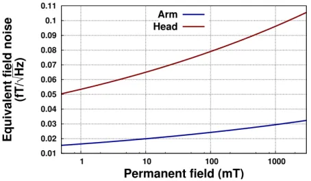
This dependence in frequency explains the need of a new evaluation of body impact at very low field. To approximate the noise generated by an arm and a full head, we model them respectively as an homo-geneous cylinder with a radius of 5 cm and an height of 5 cm and a perfect sphere with a radius of 10 cm. We consider an untuned coil ( Ø = 6 cm ) at 2.5 cm from the sample. The voltage noise emitted inside the coil will be

S1/2_V =q4kbTRbody

where T is the body temperature. This can be also written as a mag-netic field noise such as

S1/2_B =

q

4kbTRbody ω Ap

where Ap is the measuring coil area. This lead to an approximation of the generated noise (Figure1.12).

0.01 0.02 0.03 0.04 0.05 0.06 0.07 0.08 0.09 0.1 0.11 1 10 100 1000

Equivalent field noise

(fT/ √ Hz) Permanent field (mT) Arm Head

Figure 1.12: Magnetic field noise generated by an arm in a copper coil with different applied fields

We can see that around 10 mT, we expect a noise around 0.02 f T/√Hz for an arm or for a full head. The equivalent field noise dependency in volume, proportional to √V_loss, appears clearly here. This defines the lower theoretical limit we can achieve in term of noise with such MRI system.

1.2 spatial encoding and imaging features at very low field 22

1.2 s pat i a l e n c o d i n g a n d i m a g i n g f e at u r e s at v e r y l o w f i e l d

To obtain an image from the NMR signal, the use of gradients is required. In this section, three dimensional imaging is introduced through the presentation of frequency and phase encoding gradients as well as slice selection gradient. Typical sequences are presented and parameters like resolution, field of view and signal-to-noise ra-tio are precisely defined. Finally, contrast-to-noise rara-tio specificity at very low field MRI is discussed through a spin relaxation mechanisms study.

1.2.1 Frequency encoding and K-space definition

In the previous section simple methods to acquire a single NMR sig-nal have been shown. However this sigsig-nal only gives us two informa-tions about the sample :

• The number of protons which is linked to its amplitude. • Its mean relaxation properties linked to T1 and T2.

We get no spatial information straightly from the NMR signal. The use of magnetic field gradients will allow a decomposition of the signal depending on its spatial location. When we apply one linear gradient ∂Bx

∂x =Gx along~x during the acquisition, the phase shift at a position x after a time t is

∆ϕ(t) =γB0t+γGxxt

Since the signal emitted at a pixel x is proportional to the number of spins and has the phase given above, the signal detected by the coil can be written as

S(t) =

Z Z

Sampleρ

(x)ei(ω0t+γGxxt)_dx

As we will see in Chapter 2.3, the modulation factor eiω0t _{is thrown} away by the detection hardware and we define kx =γGxt such as

S(kx) = Z Z

Sampleρ

(x)eikxxdx

The result obtained after an Inverse Fast Fourier Transform is a pro-jection of our sample over x.

ρ(x) = FFT−1(S(kx))

Here kx is a coordinate in the spatial frequency space also called “K-space” in opposition to the “real” spatial space (see Figure 1.13). It

determines the spatial periodicity, also called resolution, and the field-of-view (FOV) of the acquisition. In MRI, it is more convenient to see the sampling as a function of k.

Contrasts & Large Objects Fine Details Fine Details Fine Details Fine Details Frequency Encoding Phase Encoding

Figure 1.13: K-space representation

The Fast Fourier Transform supposes a cartesian distribution of the K-space. A non-linear gradient will result in a non-cartesian dis-tribution and then a wrong image reconstruction with artifacts and distortions.

One dimensional imaging can be performed using frequency en-coding method. It can be used through a Spin Echo sequence or a Gradient Echo sequence.

(a) (b)

Figure 1.14: (a) Spin Echo and (b) Gradient Echo sequences with frequency encoding gradients along x

Gradient Echo requires an homogeneous environment as it does not use any refocusing pulse. A reverse gradient is used to refocus spins. This method is usually faster than Spin Echo as one excitation pulse is used.

1.2 spatial encoding and imaging features at very low field 24

1.2.2 Phase Encoding

The “phase encoding” dephases spins along one direction using a gradient Gy during a time τ before the acquisition. The phase shifts at a position(x, y)is ∆ϕ(t) =γB0t+γGxxt+γGyyτ Here ky=γGyτthen S(t) = Z Z Sampleρ

(x, y)eikxx+ikyydxdy

As for kx, we need to scan the K-space along y. Given that the param-eter τ is defined, this can be done by changing Gy for each ky. Thus each pixel along the second direction will require one acquisition.

Figure 1.15: Two dimensional imaging with a spin echo sequence A phase encoding can be performed on one or two directions si-multaneously. Then we can access to three dimensional imaging with a double phase encoding.

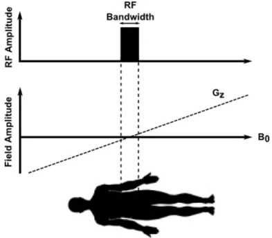
1.2.3 Slice Selection

Three dimensional imaging can also be performed slice by slice. The main idea is to excite a selective part of the sample and then to per-form a 2D imaging of this selected part. Then a three dimensional im-age can be reconstructed. A slice selection requires a pulse designed to excite a narrow frequency bandwidth ∆ f . Usually a pulse with a cardinal sinus shape is used during a time T = 1/∆ f . This specific

shape reduces the sidebands of the selection. Then if a gradient is ap-plied during this selective pulse, just a part of the entire sample will be excited.

Figure 1.16: Slice selection scheme

After the selection, a classic two dimensional imaging sequence is applied.

Figure 1.17: Three dimensional imaging with a slice selection and spin echo sequence

Working slice by slice has its advantage, even if the used pulses are longer. Further explanation will be given in Chapter 5.

1.2 spatial encoding and imaging features at very low field 26

1.2.4 Resolution

The resolution of an MRI image is defined by voxels size. It is linked to the K-space by

(kx, ky, kz) =1/δ(x, y, z)

where(kx, ky, kz)stands for a k-space line along one chosen direction and δ(x, y, z)for the resolution along the corresponding spatial direc-tion. For the frequency coding direction, we have

kx =

γGxTx 2π

where Tx is the total time of the readout gradient Gx application. Then, for a given Tx , we can achieve a resolution δx with a gradi-ent respecting

Gx= 2π δxγTx

According to this equation, we could always compensate a decrease of Tx, which corresponds to an artificial broadening of the linewidth, by an increase of Gx . However, this will lead to a larger frequency spread which leads to a decrease in signal-to-noise ratio. Moreover Tx has a maximum value which is defined by T2 or T2∗ according to external inhomogeneities. For a given δx , it is necessary to use a minimum gradient strength (see Chapter 2.2).

For the phase encoding direction, we have ky =

γNyδGyτ 2π

where Ny is the number of points along y direction and δGy one step of the phase encoding gradient. Then

δGy = 2π δyγNyτ

Just like frequency coding, τ has a maximum value which is defined by T2or T2∗.

Finally, for the slice selection direction, the resolution is defined by the pulse length and the gradient strength. A pulse with a cardinal sinus shape excites a bandwidth

∆ f = 1

t0

where t0 corresponds to one-half the width of the first lobe. For a desired resolution δz, we need a gradient such as

Gz = 2π t0γδz

1.2.5 Field Of View

The field of view is defined by the size of the spacial encoding area of the MRI image. We have

(x, y, z) =1/δ(kx, ky, kz)

where (x, y, z)stands for the field of view along one spatial direction and δ(kx, ky, kz)for the resolution along the corresponding k-space di-rection. For a frequency sampling fs= _δt1 along the frequency coding direction, we have

x= 2π

γGxδt

The frequency sampling needs to be chosen wisely to avoid any sig-nal outside this “window”. A too small field-of-view will result in wrap-around artifacts also called aliasing. Signals out of the band-width will be mismapped to the opposite side of the image leading to indecipherable images. For the phase encoding gradient, we have

y = 2π

γδGyτ

Finally, the slice selection direction doesn’t have the same field of view problematic as the image is reconstructed slice by slice and can-not be subject to any aliasing.

1.2.6 Signal to Noise Ratio

The strength of the frequency coding gradient, also called readout gradient, has an influence on the Signal to Noise Ratio. A larger gra-dient involves a larger receiver bandwidth BW and a spread of the signal which leads to an enlargement of noise contribution. Finally, the signal-to-noise ratio can be expressed as

SNR=KB0( x Nx y Ny δz) r NxNyNaverage BW

where the constant K includes detection factors (see Chapter 3 and 4), sequence parameters (TR, TE, ...) and tissues factors (body noise, spin density, T1, T2, ...), Nx and Ny are the number of frequency and phase encoding steps, Naverage is the number of signal averages and B0 the applied permanent field.

We want to compare the SNR of two identical phantoms A and B respectively sampled at B0,A =1.5 T and B0,B =10−2T with the same relative field homogeneity and the same sequence. If we call δBAand δBB the absolute field inhomogeneity between A and B, we have

δBA δBB = T ∗ 2,B T_2,A∗ = BA BB

1.2 spatial encoding and imaging features at very low field 28

where T₂∗ is the apparent relaxation time of the transverse compo-nent. We suppose here that the main external inhomogeneity is com-ing from our permanent field. This imposes conditions on gradients strength such as BWA BWB = BA BB Finally, SNRA SNRB = KA KB s BA BB ≈ 12.2KA KB

In a first approximation, Very Low Field MRI presents a reasonable disadvantage in signal-to-noise ratio in comparison to High Field MRI. With equivalent sensors in both configurations, we would lose a factor √3 12.2 ≈ 2.3 in resolution in each direction. This would cor-respond to a typical resolution of 2x2x2 mm2_{. However the ratio} KA

KB corresponding to sensors efficiency between 10 mT and 1.5 T should be equal to 1. Chapter 3 and 4 will describe new detection methods that are trying to reach this achievement. However, the signal-to-noise is not the only interesting MRI parameter.

1.2.7 Contrast-to-noise ratio

The signal-to-noise ratio and the resolution are two interconnected parameters that clearly define the quality of MRI images. However, contrast is also determinant for clinical study of images as it reveals environmental interactions and intrinsic properties of tissues. It can be defined as the relative difference of signal intensities in two ad-jacent regions A and B. It can be measured by the contrast-to-noise Ratio (CNR).

CNR=SNRA−SNRB

where SNRA and SNRB stand for the signal-to-noise ratio of both re-gions. Three main parameters can induce strong contrast differences.

The spin-lattice relaxation time T1 which depends on the lattice vibration of the sample structure. The longitudinal component Mz of the magnetic moment is relaxing such as

Mz(t) =Mz,0(1−e−t/T1)

A typical sequence to enhance contrasts between a short longitudinal relaxation time T1s and a long longitudinal relaxation time T1l is to choose a relevant repetition time TR with T1s≤ TR≤T1l and a short echo time TE to get rid of any T2 weighting. That way, for identical protons density, the sample with a short T1will reveal a higher signal. It is called a T1weighted image.

The spin-spin relaxation time T2 which depends on the random fluctuations of the local magnetic field. The transverse component Mxy of the magnetic moment is relaxing such as

Mxy(t) =Mxy,0(e−t/T2)

A typical sequence to enhance contrasts between a short transverse re-laxation time T2sand a long transverse relaxation timeT2l is to choose a relevant echo time with T2s ≤ TE ≤ T2l and a long repetition time TR to get rid of any T1weighting. That way, for identical protons den-sity, the sample with a long T2 will reveal a higher signal. It is called a T2 weighted image.

The proton density ρ which depends on tissues properties. The main difficulty of such weighted image is to suppress all other weight-ing. A long repetition time TR combined with a short echo time TE provide a pure proton density map. It has to be noticed that clinically, this type of acquisition doesn’t bring much information.

Some contrast agents are sometimes used. After oral or intravenous administration, they enhance the contrast-to-noise ratio of specific tis-sue lesions. Very low field MRI present strong particularities about relaxation time. The Bloembergen-Purcell-Pound (BPP) theory [8] pro-poses a 2-spin system model with a rotational movement character-ized by the correlation time τCof the molecular tumbling motion. Ac-cording to this model, the relaxation times T1and T2of such molecule depends on the Larmor frequency in the following way :

1 T1 =K[ τC 1+ω₀2τ_C2 + 4τC 1+4ω2₀τ_C2 ] 1 T2 = K 2[3τC+ 5τC 1+ω2₀τ_C2 + 2τC 1+4ω2₀τ_C2 ]

where ω0 is the Larmor frequency and K a constant depending on the molecule.

Figure 1.18: Dependency of T1and T2on the Larmor pulsation ω0according

to the BPP theory

The correlation time τCfor H2O molecules is typically around 10−12 seconds in liquid phase without contamination. In vivo, water is

1.2 spatial encoding and imaging features at very low field 30

bounded to macromolecules and the correlation time ranges from 10−9 to 10−6 seconds [27]. When ω_{0  τc}, it appears that T₂ and T

1 tend to the same value. It has been verified experimentally for brain tissues [58]. Grey matter at 1.5 T Grey matter at 46 µT White matter 1.5 T White matter 46 µT T1 1130ms 103± 5ms 889ms 75±2ms T2 102ms 106±11 ms 86ms 79 ±11ms

Table 1.2: Relaxometry of brain tissues at high field and at ultra low field

[58]

We can also notice that both T1and T2become more sensitive to the correlation time τC. This parameter related to macromolecules motion brings a new specific information contained inside T1and T2. In [33], the T1 of two samples with different concentration of agarose ( and then a different τC ) are monitored at different frequencies. It appears that below 10 mT, their longitudinal relaxation time is diverging. The result is the apparition of new contrasts at those frequencies.

Figure 1.19: Relaxation rate dispersion of 0.25% and 0.5% agarose gel in

wa-ter measured between 72 Hz and 12.8 MHz.[33]

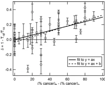
A clinical application of this relaxation change has been studied concerning the prostate cancer. S. Bush and al. [10] have recently shown in ex-vivo prostate that cancerous tissues were presenting a different T1 than normal tissue at low frequency.

Figure 1.20: Contrast δ versus the percentage cancer between two ex-vivo

prostate A and B. The solid line fit respect y=0.003x and R2=

0.3 . The dashed line fit respect y=0.0036x−0.0334 and R2=

0.31.[10]

Intrinsically, very low field MRI presents a lower signal-to-noise ratio than high field MRI. However contrasts at those frequencies are more sensitive to some biological environment properties and could then lead to new diagnosis possibility.

c o n c l u s i o n

Very low field MRI relies on the same principle than high field MRI but important differences have been enlightened. The polarization of the nuclear magnetic moment is much smaller but its impact on signal-to-noise ratio is compensated by a reduced acquisition band-width due to a better absolute homogeneity. Thus a factor 2.3 in reso-lution is lost for every direction in comparison to 1.5 T devices. More-over, the frequency of the nuclear magnetic relaxation is much lower which implies difficulties for the detection. It will be precisely devel-oped in Chapter 3 and 4. Regardless of the sensor, the fundamental noise limit is related to the magnetic noise generated by the body. At very low field, this noise has a lower amplitude as the conductivity of biological tissues is decreasing with frequency. With ideal sensors, we would then lose only a factor 1.8 in resolution in comparison to 1.5T devices. Finally, this loss could be balanced by a better contrast-to-noise ratio due to molecular motion influence on T1 below 10 mT.

2

Full-head setup for MRI at very low field

agnetic Resonance Imaging uses a complex combina-tion of fields. Each one of them must be precisely defined in terms of amplitude, frequency, homogeneity and timing. Therefore a com-plete study of needed components is necessary to achieve a correct acquisition. From gradients to radio-frequency pulses including spec-trometer and permanent field, all of them will be designed and then tested to fulfill very low field requirements. The methodology and results will be presented through three different sections.

2.1 p e r m a n e n t f i e l d a n d h o m o g e n e i t y

In this section, permanent field is discussed. Different methods are explored to generate a field with an amplitude and homogeneity adapted to very low field MRI. Two setups are described :

• One existing setup adapted for small objects imaging [18] • One new setup adapted for full-head imaging

The design of both configurations is described and a precise charac-terization of all relevant parameters (amplitude, homogeneity, noise) is performed.

2.1.1 Different kind of magnets

In MRI, several options exist to generate a magnetic field.

Superconducting electromagnetsare the most common devices for clinical MRI with a field above 1.5 T. Superconducting material like niobium-titanium or niobium-tin are used to wind the coil. Those ma-terials lose their resistance below their critical temperature (around 10 K). When the alloy is cooled by liquid helium to 4K, it thus becomes superconductor. This important physical effect will be explained more precisely in Chapter 3. Without resistance, an important current can flow through the coil and generate a high field with a good stabil-ity. However those magnets are extremely costly to produce and the cryogenic helium is expensive and difficult to handle for such sized coils. Their cylindrical geometry also imposes a confined space for the patient which can induced claustrophobia problem.

Permanent magnet are conventional magnets made of ferromag-netic materials containing steel alloys with rare earth elements. Com-pared to superconducting magnets, they generate a weak field (usu-ally≤ 0.4 T) which is limited in precision and stability. Moreover, it is impossible to adjust accurately the field or to “turn off” those mag-nets. Finally, reaching such field strength requires large and bulky elements that can weight over 100 tonnes. Even if they are inexpen-sive to maintain, those magnets are not easy to use for clinical MRI.

2.1 permanent field and homogeneity 34

(a) (b)

Figure 2.1: a) 3 T MRI system with superconducting electromagnets (SIEMENS) and b) 0.35 T MRI system with permanent magnets (NEUSOFT)

Resistive electromagnetsare very similar to superconducting mag-nets in term of design. The coil is a solenoid wound from copper. Field strength and stability of such electromagnet are limited and re-quire an important electrical energy during operations. However it is a relevant method for very low field MRI applications. The initial cost is low and it is possible to build open and light systems to generate a field as high as 10 mT with a good homogeneity. This is the solution that has been chosen for our very low field MRI system.

2.1.2 Homogeneity required

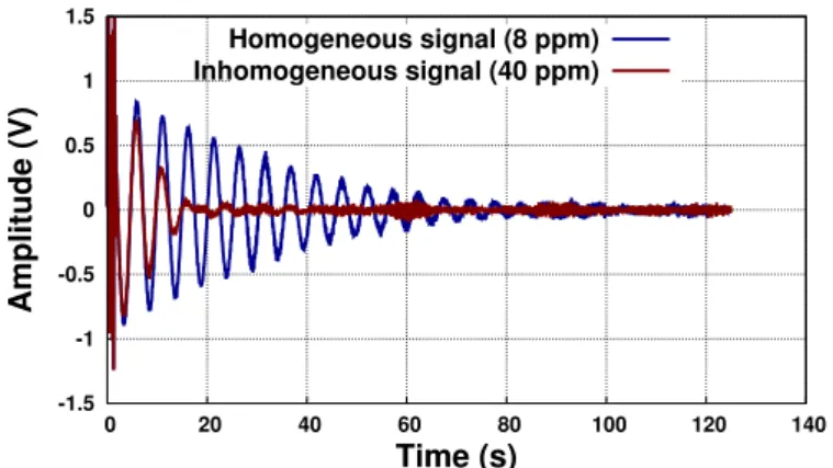
The homogeneity of the permanent field B0is of primary importance for MRI applications. For a magnetic field variation of δB on a sample, we have 1 T₂∗ = 1 T2 + 1 2πγδB

Then T₂∗ can be defined as the relaxation time due to spin-spin re-laxation and all external magnetic field inhomogeneities. Spins in-side the sample will present different precession frequencies and will move out of phase much faster. Then

T₂∗ ≤T2

This relaxation time defines the linewidth at half-height δv of our NMR signal such as

δv= 1 T₂∗

-1.5 -1 -0.5 0 0.5 1 1.5 0 20 40 60 80 100 120 140 Amplitude (V) Time (s) Homogeneous signal (8 ppm) Inhomogeneous signal (40 ppm)

Figure 2.2: Free induction decay of two NMR signals in two different inho-mogeneous fields.

Reducing the linewidth to its minimum intrinsic value _T21 is use-ful to perform images with a good resolution on a small bandwidth acquisition. Then we should always try to reach

δB≤ 2π γT2

In biological tissues , spin-spin relaxation time T2 are of the order of 50 ms or less [3] which gives us δB ≤ 0.47µT. For Very Low Field MRI ( 1 mT to 10 mT ), this corresponds to a maximum homogeneity of 47 ppm. Based on those observations, two setups of different size have been used.

2.1.3 Coils design

The conception of an homogeneous field is a difficult problem which requires a specific mathematical framework. Based on the work of Roméo and Hoult [49], a simplistic introduction of the usual methods to perform such field optimization is presented here.

2.1 permanent field and homogeneity 36

In a volume through which no current passes, we know that a mag-netic field~B respects Laplace equation such as

~

∇2~B=0

Solutions of this equation in a spherical polar coordinates can be ex-pressed as spherical harmonics of the form

Tnm =CnmrnPnmcosθ     sin mΦ cos    

where Cnm are constants, Pnmcosθ are Ferrer’s associated Legendre functions and n > m > 0 . Then any field generated by a current element can be expressed as a sum of spherical harmonics. It is then possible to think about relevant combination of current element in order to eliminate unwanted spherical harmonics while enhancing the harmonics of interest (n, m= 0, 0 in the case of an homogeneous field). This optimization of the field should always respect physical constrains of size and weight. Moreover the presence of unavoidable higher-order harmonics places an upper limit upon the volume over which the field is considered as a single harmonic.

2.1.4 Small size setup

This setup was build during Hadrien Dyvorne’s thesis [18]. The ge-ometry chosen for the small size setup is a rescale version of a magnet system for Low-Field Electron Paramagnetic Imaging imaging used by Rinard and Al [48]. This set of four coils have been optimized to ideally cancel unwanted harmonics until the 8th order.

(a) (b)

Figure 2.4: a) Four-coil magnet that generates a permanent field B0along z

axis and b) its magnetic field amplitude map in 2D using a finite element method simulation for a current of 10 A(FEMM 4.2) This four-coil magnet design has been chosen as it is offering a large volume of magnetic field homogeneity for a rather compact and

open system compatible with the use of a cryogenic dewar. The two large inner coils CLand the two small outer coils CS are supplied by the same current, circulating in the same direction. Precise character-istics of each coil are described in Table2.1.

Coil Number of

Turns Wire Section Turns/Layer Total Section

CL 120 2*6.5mm2 5 48*32.5mm2

CS 30 2*6.5mm2 3 20*19.5mm2

Table 2.1: Winding parameters for the four-coil magnet

A finite element method software ( FEMM 4.2 ) [15] is used to predict the generated magnetic field. Coils material, size, position and section are taken into account to obtain the Figure2.5. The simulation is obtained for a circulating current of 10 A. It should be noticed that the final homogeneity depends also on the winding procedure which is considered as negligible in this ideal model.

5.33598 5.336 5.33602 5.33604 5.33606 5.33608 5.3361 5.33612 -3 -2 -1 0 1 2 3 Magnetic field B 0 (mT)

Distance from center (cm)

Figure 2.5: B0simulated profile along z axis for a current of 10 A

The simulation predicts a magnetic field per unit current around B0 ≈ 5.33 G/A with an homogeneity of 20 ppm over a 5 cm x 5 cm x 5 cm square sample. Coils are supported by a non magnetic aluminum structure. This metallic material could be sensitive to field change (see Chapter 2.2) but with a permanent polarization, no Eddy currents are created. Moreover, the magnetic noise coming from the thermal noise inside the aluminum has been evaluated and is less than 0.4 f T/√Hz.

A stable and low noise power supply is needed to achieve the the-oretical homogeneity of 20 ppm. A DC supply Delta 1500W (model SM 35-45) has been chosen. It is well adapted given that the four-coil system has a total a resistance around 1Ω.

2.1 permanent field and homogeneity 38 Maximum voltage Maximum current Current stability Ripple current noise 35V 45A 9∗10−5 A/h 15 mA

Table 2.2: Delta SM 35-45 characteristics

In Table 2.2, the peak to peak ripple current noise is measured on a bandwidth of 50 MHz. It is rather high and it leads to an important homogeneity degradation. A 20 ppm homogeneity at 10 mT requires an equivalent ripple current noise of 380 µA or lower. The main part of this ripple noise comes from 50 Hz and 100 kHz harmonics (MOS-FET power conversion frequency).

Figure 2.6: RC Filter to minimize power supply ripple current noise A RC filter (Figure 2.6) is added to the power supply to filter those perturbation. The ripple current noise is divided by a factor 20 (≈ 760µA ≡ 40 ppm). At 1 mT, this current perturbation involves a degradation of the homogeneity up to 400 ppm. It remains the main limitation of our permanent polarization and the current drift of 9∗10−5A/h is negligible even for long acquisition time (.8 hours). 2.1.5 Full size setup

This particular system has been planed to be able to make in-vivo imaging of a human brain. The design has been chosen with the help of a private company Cedrat. It was necessary to have a rather good homogeneity on a large volume with an open and compact geometry. The patient-friendliness criteria was defined as a large free area in his field of view in order to minimize enclose feelings and subsequent claustrophobic effects. It has been assume that a 90° free vision angle was sufficient.

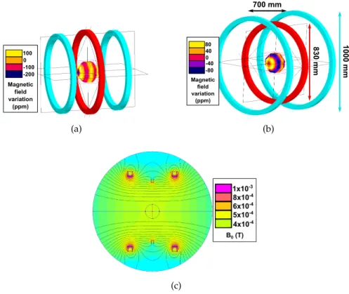
Figure 2.7: Schematic of the proposed patient-friendly structure A three-coil Maxwell configuration was first proposed but it was not respecting the patient-friendliness criteria. The height of this con-figuration was modified to fulfill this condition and then the central coil size and Ampere-turn in each coil were optimized to reach the best homogeneity at 10 mT (see Figure 2.8). The configuration has been built horizontally for a better ease of use but could be adapted vertically. 100 0 -100 -200 Magnetic field variation (ppm) (a) 1000 mm 830 mm 700 mm 80 40 0 -80 -40 Magnetic field variation (ppm) (b) (c)

Figure 2.8: a) Classic coil Maxwell configuration b) Optimized three-coil configuration and c) its finite element method simulation of

B0

The entire structure to maintain the coil is in wood which excludes all parasite effects of conducting material like Eddy currents or extra

2.1 permanent field and homogeneity 40

magnetic noise. The same current is applied on both external coils, in the same direction. The current circulating in the central coil is lower but also in the same direction. The ratio is

Ratio= Icentral

Iexternal

=0.56

The considered working zone is a sphere with a diameter of 20 cm at the center of the structure. The total winding mass is around 180 Kgs and an integrated cold loop provide efficient cooling for the dis-sipated power (1,4 kW).

Coil Wire

diameter

Number of

turns Total section

Central 1.4 mm 72 35*35 mm

External (data

for 1 coil) 1.4 mm 280 65*65 mm

Table 2.3: Winding parameters for the three-coil magnet

A finite element method simulation is performed again with a cur-rent of 1 A (Figure2.8). A magnetic field profile is measured along x in the working zone (Figure2.9).

4.0008 4.001 4.0012 4.0014 4.0016 4.0018 4.002 4.0022 -10 -5 0 5 10 Magnetic field B 0 (Oe)

Distance from center (cm)

Figure 2.9: Magnetic field B0profile along x

On a sphere of 10 cm radius, the FEMM simulation predicts a mag-netic field around B0 ≈ 5.3 G/A with an homogeneity of 150 ppm with a perfect current source. The real current source brings some more perturbations that need to be taken into account. For the total resistance of 3.588Ω, a Delta 1500 W (SM 70-22) has been chosen.

Maximum voltage Maximum current Current stability Ripple current noise 70V 22A 9∗10−5A/h 10 mA

Another RC filter has been added to the power supply to filter the ripple current noise.

Figure 2.10: RC Filter to minimize power supply ripple current noise

2.1.6 Measurements of strength and homogeneity

Nuclear Magnetic Resonance is a powerful tool to evaluate magnetic field properties. For both setup, the same procedure has been used to measure the strength of the magnetic field B0 and its homogene-ity. A sample, corresponding to the working volume of the system, is positioned at the center and filled with pure water : a square of 5x5x5 cm3 for the small setup and a sphere with a radius of 15 cm for the full-head setup. A tuned coil is used here as detection with a resonance frequency of 300 kHz for the small setup and 190 kHz for the full-head setup. Our first experiment is to find the current to generate a field corresponding to the Proton Larmor Frequency adapted to the tuned coil. A single π

2 pulse is applied on the sample with a repetition time of 1 second. For a precise value of current, an NMR signal should appear at 300 kHz (or 190 kHz for the full-head setup) on our monitoring devices (see Chapter 2.3). This gives us a precise measurement of the signal strength in function of the current circulating in the coils.

Magnetic Field Strength Predicted

Magnetic Field Strength Measured

Small Size Setup 5.1 G/A 4.6 G/A

Full Size Setup 5.3 G/A 4.7 G/A

Table 2.5: Magnetic field strength of both experimental setup

As we have seen before, the inhomogeneity inside a sample is trans-lated into a transverse relaxation time change. This relaxation can be directly measured by the half-height linewidth of the NMR signal Fourier Transform. It is of prime importance to use a sample with a long T2 (≥ 250ms) to avoid any intrinsic transverse relaxation limita-tion. The small setup has been tested at 7 mT and the full size setup has been tested at 4.4 mT. A spherical phantom has been used for the full-head setup. In both setup, the Free Induction Decay width has

2.1 permanent field and homogeneity 42

been measured for 1 acquisition and for 300 averaged acquisitions to evaluate the current supply noise impact.

-0.8 -0.6 -0.4 -0.2 0 0.2 0.4 0.6 0.8 0 50 100 150 200 Amplitude (V) Time (ms) 300 acquisitions 1 acquisition (a) 20 Hz 4 Hz (b)

Figure 2.11: Inhomogeneity measurements in the small size setup for one acquisition and 300 acquisitions. a) The Free Induction Decay and its b) Fourier Transform.

The half-height linewidth can then be translated into an inhomo-geneity level. The difference between the measurement for one acqui-sitions (4 Hz) and 300 acquiacqui-sitions (20 Hz) comes mainly from the ripple current noise coming from the current supply. Those punctual variations participate to the widening of the peak.

-1 -0.5 0 0.5 1 1.5 2 0 5 10 15 20 25 30 Amplitude (V) Time (s) (a) 114 Hz (b)

Figure 2.12: Inhomogeneity measurements in the full-head setup for 300 ac-quisitions. a) The Free Induction Decay and its b) Fourier Trans-form.

For the full-head setup, no differences were measured for one ac-quisition or 300 acac-quisitions. It corresponds to a linewidth of 114 Hz. All results are combined in Table2.6.

Linewidth for 1 acquisition Inhomogeneity for 1 acquisition Linewidth for 300 ac-quisitions Inhomogeneity for 300 acquisitions Small size setup (7 mT) 4Hz 8.5 ppm 20Hz 42.5 ppm Full size setup (4.4 mT) 114Hz 600ppm 114Hz 600ppm

Table 2.6: Inhomogeneity measurements

Any MRI acquisition requires averaging. Thus the relevant inho-mogeneity measurement is given after 300 acquisitions. It should be pointed out that the small setup was tested in different environments : a classic laboratory and a non-magnetic building. No differences were measured after 300 acquisitions confirming that the current supply is the main limitation here.

The inhomogeneity measured for the full size setup is much larger than the simulation. It is mainly due to an error in the Ampere-turn ratio between the central coil and external coils. It has been compen-sated using parallel resistances but the precision is limited.

2.2 gradients and rf pulses 44

2.2 g r a d i e n t s a n d r f p u l s e s

Linear gradients are essential for precise MRI acquisitions. The re-quired strength and linearity needed for very low field applications are discussed here. Three different gradient designs are presented. Each one of them is adapted to one particular MRI setup. Their geom-etry is described and a characterization of their strength and linearity is also given. Finally, an RF coil design is proposed to fulfill precise requirements previously defined. Its homogeneity is then experimen-tally measured.

2.2.1 Gradient specificity

Unlike permanent field, gradients need to be switch off and on dur-ing an MRI acquisition and require reasonable amplitude. At high fields, gradients amplitude up to 100 mT/m can be used. For those reasons, resistive electromagnets are perfect candidates to generate such fields. An important drawback of those gradients at high field is the acoustic noise. The alternation of currents in the presence of the strong static field produces significant Lorentz forces that act upon the gradient coils. Then motion and vibration of gradients generate an acoustic noise typically around 90 dB. But those noises depend on the strength of gradients. At low field, their amplitude is lower and so is the resulting acoustic noise. Moreover, currents alternation often comes with Eddy currents which implies dedicated active screening for such gradients to minimize perturbations. This problem is also greatly reduced at low fields.

In both developed setup, gradients are also used as active shim-ming coils. Permanent external inhomogeneity can be compensated by sending a DC current inside coils.

2.2.2 Gradient strength and linearity required

The gradient strength G is determined by the resolution δr we want to achieve in addition to the fundamental linewidth δv of our NMR signal. As we have already seen in Chapter 1.2,

G= 2π

δrγT₂∗ = 2πδv

δrγ

We understand here the importance of a good homogeneity. A low amplitude gradient sharpens the acquisition bandwidth, increases the signal-to-noise ratio, lowers the acoustic noise and reduces par-asite eddy currents. The relative homogeneity at low field is approx-imately the same as at high field. It means that we have a linewidth 150times lower at 10 mT if we neglect the intrinsic linewidth of our

product (100 ms≈10 Hz). We should then require a gradient ampli-tude around 1 mT/m.

Another important point is linked to the linearity of gradients. Due to the reconstruction pattern (Fast Fourier Transform), a cartesian ac-quisition of the K-space is extremely important to obtain a correct image.

(a)

(b)

x

x

G

G

x

x

A

A

Figure 2.13: (a) Two similar square samples are acquired in one dimension along x with two different gradients. (b) The resulting images are given for the linear and the non linear gradient.

Any deviation from a perfect linear gradient will result in a defor-mation of our image. At a point (x,y,z), the non-linearity δGnorm(x, y, z) of a gradient is defined as the normalized difference between its ac-tual value and its ideal value

δGnorm(x, y, z) =

B(x, y, z) −B_ideal(x, y, z)

Bideal(x, y, z)

The parameter we are considering is the maximum absolute value of this non-linearity on the working volume | δGnorm |max. Most of the time, this maximum concerns the surface of the working volume. It is important to notice that gradients non-linearity is not a random perturbation like regular noises. On one hand it means that gradients non-linearity will always dominate the background external noise at some point after enough averaging. On the other hand some recon-struction algorithms can be used to compensate an important δGnorm. The optimization of such field is based on the same principle than for a permanent field. However, the relevant harmonic corresponds to n, m=1, 0 for a linear gradient.

2.2.3 Small size setup

A specific geometry has been chosen to satisfy the problematic of this small size setup. Because of the screening effect of the aluminum frame of the B0 coils, the gradients have to be placed between the permanent coils structure. The main field homogeneity of 47 ppm at

2.2 gradients and rf pulses 46

10 mT imposes a minimum amplitude limit. A gradient strength as high as 0.4 mT/m to reach a 1 mm resolution is required. The three directions gradients are generated by using two different coil design.

(a) (b)

Figure 2.14: (a) Gradient field along Z and (b) the FEMM simulation

Circular Maxwell coils are used to create the gradient field along z direction. The cancellation of harmonics until the fourth order is obtained if their centers are spaced by a distance d = R√3 where R is the coil radius. A finite element method simulation is performed with FEMM 4.2 to determine our linearity and strength.

d R Number of turns Z gradient strength Gradient linearity 180mm 104mm 30 2.2 mT.m−1.A−1 9.10−3

Table 2.7: Parameters of the Maxwell coils for the small size setup

Z0 = 180 mm w = 132 mm Y0 = 520 mm x = 68 mm Y Z X

Figure 2.15: Gradient coils to encode along direction X (dark blue) and Y (light blue).

Rectangular planar coilsare used to create the gradient fields along x and y directions. Inspired by [5], those gradients are perfectly adapted to the small size geometry as the central zone remains easily accessi-ble. A simulation using FLUX [1] is performed.