Experimental study of dense suspension flow under cone-plate device

(1)

HAL Id: tel-01562493

https://tel.archives-ouvertes.fr/tel-01562493

Submitted on 15 Jul 2017

HAL is a multi-disciplinary open access archive for the deposit and dissemination of sci-entific research documents, whether they are pub-lished or not. The documents may come from teaching and research institutions in France or abroad, or from public or private research centers.

L’archive ouverte pluridisciplinaire HAL, est destinée au dépôt et à la diffusion de documents scientifiques de niveau recherche, publiés ou non, émanant des établissements d’enseignement et de recherche français ou étrangers, des laboratoires publics ou privés.

Experimental study of dense suspension flow under

cone-plate device

Wei Zhu

To cite this version:

Wei Zhu. Experimental study of dense suspension flow under cone-plate device. Fluids mechanics [physics.class-ph]. Ecole Centrale Marseille, 2016. English. �NNT : 2016ECDM0007�. �tel-01562493�

(2)

ECOLE CENTRALE DE MARSEILLE

ED 353 – SCIENCES POUR L’INGENIEUR : MECANIQUE, PHYSIQUE,

MICRO ET NANOELECTRONIQUE

IRPHE UMR 7342, Equipe Biomécanique

Thèse présentée pour obtenir le grade universitaire de docteur

Discipline: Mécanique et Physique des fluides

Wei ZHU

Experimental study of dense suspension flow under

cone-plate device

Soutenue le 14/10/2016 devant le jury :

Cécile LEGALLAIS, Directrice de recherche CNRS, BMBI, Compiègne, Rapporteur Stéphane NOTTIN, Maître de Conférences, Univ d’Avignon, LaPEC, Rapporteur Nadine CANDONI, Professeur Aix-Marseille Université, CINaM, Examinatrice Valérie DEPLANO, Directrice de recherche CNRS, IRPHE, Directrice de thèse Yannick KNAPP, Maître de Conférences, Univ d’Avignon, Co-directeur de thèse

(3)

1

Résumé

Par rapport à un fluide Newtonien, les suspensions denses de particules présentent des propriétés rhéologiques différentes. Des comportements rhéofluidifiants ou rhéoépaississants lié à des phénomènes de migration de particules peuvent apparaitre. Pour des suspensions, le taux de cisaillement, la concentration et la taille des particules ont une grande influence sur ce comportement rhéologique (Denn et Morris 2014). Pour observer l'influence de ces facteurs, l'un des meilleurs moyens est de disposer d’un système simple dans lequel tous les facteurs mentionnés ci-dessus sont bien contrôlés. Ceci peut être réalisé par le développement d'une plate-forme expérimentale, sur laquelle les comportements d'écoulement de suspension (profil de vitesse et concentration locale de particules) à des vitesses de cisaillement et des concentrations de particules bien contrôlées peuvent être étudiés.

Dans l'étude actuelle, 4 tâches ont été réalisées:

1) Le développement d'une nouvelle formulation pour la préparation d’une suspension adaptée en indice de réfraction et en densité basée sur des particules de PMMA.

2) Le développement d'un dispositif expérimental consacré à l'étude des flux de suspension dense sous une large gamme de taux de cisaillement constant.

3) La caractérisation des profils de vitesse des flux de suspension dense sous un dispositif cône-plan utilisant des techniques de micro-PIV.

4) Une mesure préliminaire de la concentration locale de particules de la suspension sous écoulement cône-plan en utilisant des méthodes de traitement d'image.

Mots clés : suspension, rhéologie, adaptation de l’indice de réfraction et de la densité,

(4)

ii

Abstract

Compared to general Newtonian fluids, highly concentrated mixtures of particles and fluid, so called dense suspensions, have different rheological properties and fluid dynamic behaviors. Such as, shear-thinning or shear-thickening effect, and apparent slip and particle migration behaviors under certain shear flow conditions. These properties are related to the application of suspension flow in real systems, for example, the blood. For suspensions, shear rate, particle concentration and particle size have a big influence of on their rheological behaviors (Denn and Morris 2014). To observe the influence of these factors, one of the best ways is to start the research from a simple case in which all the above mentioned factors are well controlled. This can be realized by developing such an experimental platform, on which the suspension flow behaviors (velocity profile and local particle concentration) at different shear rates and particle concentrations can be investigated.

In the current study, 4 tasks were achieved:

1) The development of a new recipe for the preparation of density and refractive index matched suspension with PMMA particles.

2) The development of an experimental set-up devoted to the investigation of dense suspension flow under a large range of constant shear rate.

3) The characterization of the velocity profiles of dense suspension flows under a cone-plate device by using micro-PIV techniques.

4) A preliminary measurement of the local particle concentration of the suspension flow by using image processing techniques.

Keywords: suspension, rheology, refractive index and density matching, micro particle

(5)

iii

Acknowledgements

In the study of my thesis, I thank all the people who have helped me and encouraged me. My deepest gratitude goes first and foremost to my co-director Yannick Knapp, for his constant encouragement and guidance. He has walked me through all the stages of the work of this thesis. Without his consistent and illuminating instruction, this thesis could not have reached its present form.

Secondly, I would thank my director Valérie Deplano, who has shown much patience to help me to improve my presentation skill, and to help me to develop a rigorous academic habit.

Besides my advisors, I would like to thank the rest of my thesis committee: Dr. Cécile Legallais, Prof. Nadine Candoni, and Dr. Nottin Stéphane, for their insightful comments and encouragement, but also for the hard question which incented me to widen my research from various perspectives.

I thank Eric Bertrand, who helped me to make some experimental components and to fix some problems of the experimental set-up. I thank also Massimiliano Rossi, who gave me his code and some useful consultant on image processing.

Last, my thanks would go to my family for their loving considerations and great confidence in me all through these years. Especially, my mother keeps supporting and encouraging me in all the tough moments. I also owe my sincere gratitude to my friends, Rizqie Arbie, Medamine Chetoui, Adam Scheinherr, Kaili Xie, Zhuang Pei, Jun Chen, Zhanle Yu, Wen Ou, Rui Liu, Kailang Liu and Wei He, who gave me their help and time in listening to me and helping me work out my problems during the difficult course of the thesis.

(6)

iv

List of figures

Fig 2.1 Conceptual classification of the rheophysical regimes of a suspension as a function of shear rate

and solid fraction on a logarithmic scale (Coussot and Ancey 1999). ... 7

Fig 2.2 Relative viscosity vs. particle volume fraction predicted by Einstein's equation for dilute hard-sphere suspensions (Equation (2.6) with B = 2.5), and Krieger–Dougherty's equation for concentrated hard-sphere suspensions (Equation (2.9) with ϕm = 0.6). ... 10

Fig 2.3 Representation of relative viscosity versus shear rate for a fluid suspension (Stickel and Powell 2005). ... 11

Fig 2.4 Illustration of the alignment of the suspended particles following the flow direction (a) compared to the initial disordered state (b) ... 12

Fig 2.5 1.25μm PVC particles in dioctyl phthalate (R. L. Hoffman 1972) ... 13

Fig 2.6 Variation of critical shear rate with respect to ... 13

Fig 2.7 “Phase diagram” for suspension rheology, based solely on a dimensional analysis (Stickel and Powell 2005). ... 14

Fig 2.8 Contour plot of particle pair relative flux, for = 31.5%: a) Re = 0.1, b) Re = 10. (Picano et al. 2013) ... 15

Fig 2.9 Instantaneous configurations of transient clusters in the shear thickening regime, observed using fast confocal microscope. Different colors indicate different clusters. Particles outside the large clusters are drawn with smaller size for clarity (Cheng et al. 2011). ... 15

Fig 2.10 Variations of blood viscosity under different conditions as a function of shear rate (Chien 1970) 18 Fig 2.11 Rouleaux of human red cells photographed on a microscope slide showing single linear and branched aggregates (left part) and a network (right part). The number of cells in linear array are 2, 4, 9, 15, and 36 in a, b, c, d, f, respectively (Fung 1993)... 18

Fig 2.12 Schematic illustration of parallel shear plates ... 20

Fig 2.13 Schematic illustration of Couette cell device ... 21

Fig 2.14 Schematic illustration of rotational parallel disks ... 21

Fig 2.15 Schematic illustration of cone-plate ... 22

Fig 2.16 Schematic illustration of capillary and micro channel ... 22

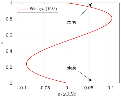
Fig 2.17 Normalized radial velocity profile of the theoretical deduction of Sdougos et al.(1983). Here u positive represents outward radial movement. ... 24

Fig 2.18 Schematic presentation of different boundary conditions: a) no-slip, b) true slip and c) apparent wall slip (Korhonen et al. 2015). ... 26

Fig 2.19 Layering of particle near the wall in concentric cylindrical Couette cell (Blanc et al. 2013) ... 27

Fig 2.20 Concentration profiles measured across the gap between rotating concentric cylinders using magnetic resonance imaging for suspensions with mean values of ϕ=0.58 (squares), 0.59 (circles), and 0.60 (triangles). (Ovarlez, Bertrand, and Rodts 2006)... 29

Fig 2.21 Variation of the shear rate across the gap between rotating concentric cylinders, data source from (Ovarlez, Bertrand, and Rodts 2006) ... 29

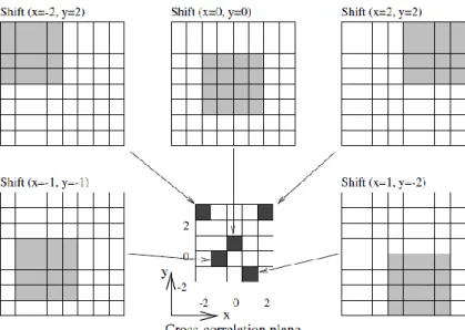
Fig 2.22 Schematic illustration of a micro-PIV set-up (Lindken et al. 2009) ... 31 Fig 2.23 An example of the formation of the correlation plane by direct cross-correlation: here a 4×4 pixel

(10)

viii

template is correlated with a larger 8×8 pixel sample to produce a 5×5 pixel correlation plane (Raffel et al.

2007a) ... 32

Fig 2.24 Peaks in a cross-correlation map with different shift distances, and represent the shift in the x and y directions respectively (Raffel et al. 2007a)... 33

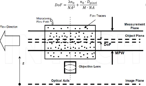
Fig 2.25 Schematic illustration of depth of focus and measurement plane width (Koutsiaris 2012) ... 34

Fig 2.26 Optical geometry used in deriving the particle image diameter (Rossi et al. 2011) ... 39

Fig 2.27 Schematic representation of the cross section of particle image intensity for different z-position based on equation (2.42) and (2.44), the particle image diameter increases for increasing z, while the peak intensity decreases. The dashed line represents the geometrical spreading of an image of out of focus particle (Kloosterman, Poelma, and Westerweel 2010). ... 41

Fig 2.28 Illustration the position of a particle in the Cartesian coordinate based on the image plane ... 42

Fig 2.29 GDPT working principle: a target particle image is compared to a set of calibration images by using the normalized cross correlation. The out-of-plane coordinate for the target particle is found where the maximum correlation is the highest as a function of the out-of-plane coordinate Z (Barnkob, Kähler, and Rossi 2015). ... 44

Fig 3.1 Viscosity variations of 41μm particle suspensions at different concentrations with respect to shear rate. (The viscosity of the 2% 41μm particle suspension is not shown since it is too close to that of 0%. All the error bars are removed as they are too small compared to the minimum scale.) ... 58

Fig 3.2 Viscosity variations of 4.62μm particle suspensions at different concentrations with respect to shear rate. (The viscosity of the 2% 4.62μm particle suspension is not shown since it is too close to that of 0%. All the error bars are removed as they are too small compared to the minimum scale.) ... 59

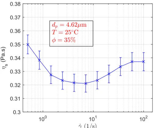
Fig 3.3 Viscosity variation of 4.62μm particle suspension at =35% with respect to shear rate ... 60

Fig 3.4 Viscosity variation of 4.62μm particle suspension at =45% with respect to shear rate ... 60

Fig 3.5 Relative viscosities of 41μm particle suspensions at different shear rates as a function of particle concentration, where =0.582 is taken for the Krieger-Daugherty model. ... 61

Fig 3.6 Relative viscosities of 4.62μm particle suspensions at different shear rate as a function of particle concentration, where =0.596 is taken for the Krieger-Daugherty model. ... 62

Fig 3.7 “Phase diagram” for suspension rheology, based solely on a dimensional analysis. Image source from (Stickel and Powell 2005). ... 64

Fig 3.8 Relative viscosities of 4.62μm and 41μm particle suspensions at concentration of 45% compared to the relative viscosities of blood measured by Chien (1970) and Whitmore (1968) as a function of shear rate. ... 65

Fig 4.1 Illustration of the components under the cover ... 68

Fig 4.2 Illustration of the experimental set-up ... 68

Fig 4.3 Schematic illustration of the cone-plate device ... 69

Fig 4.4 Schematic illustration of the measured region in the x-y plane ... 69

Fig 4.5 Velocity profile (a) and the normalized velocity profile (b) of the flow under the cone-plate device with no slip and no secondary flow ... 70

Fig 4.6 Cover, temperature control module and foam cushion ... 72

Fig 4.7 An example of multi-plane of velocity fields and the generation of the corresponding velocity profile ... 73

Fig 4.8 Schematic illustration of the light path in the experimental set-up ... 74

Fig 4.9 Illustrations of the measured and ... 74

Fig 4.10 Variations of the vector length (v) as a function of image pair of 0% and 20% 41µm particle suspension at 50 s-1_{and at H=524µm. ... 79}

(11)

ix

Fig 4.11 Illustrations of secondary flow in a cone-plate device, a) the flow direction of secondary flow, b)

illustration of the velocity vector near the cone surface and near the plate surface ... 80

Fig 4.12 Normalized velocity profiles of 0% particle suspension at: a)100s-1_{, 50s}-1_{and 10s}-1_{, b) 5s}-1_{, 1s}-1_and 0.5s-1_{. ... 81}

Fig 4.13 Normalized radial velocity profile of the theoretical deduction of Sdougos et al.(1983), and normalized radial velocity profile of the 0% particle suspension at 100s-1_{, here u positive means outward} radial movement. ... 82

Fig 4.14 u/v ratio based on the theoretical deduction of Sdougos et al.(1983), and of the 0% particle suspension at 100s-1_{, here u positive means outward radial movement. ... 82}

Fig 4.15 Schematic illustration of the local particle concentration measurement principle, where H is the measured height, the measurement plane width is 2d which will be described in section (4.4.3). ... 84

Fig 4.16 Illustrations of the particle position locating procedures ... 86

Fig 4.17 Illustration of the image calibration and z-position determination in measurement ... 87

Fig 4.18 Illustrations of the particle positions for local particle concentration calculation ... 88

Fig 5.1 Normalized velocity profiles of 41μm particle suspensions at =45%, 35%, 20% and at 10s-1_{. ... 90}

Fig 5.2 Normalized velocity profiles of 4.62μm particle suspensions at =45%, 35%, 20% and at 10s-1_{. .. 90}

Fig 5.3 Normalized velocity profiles of 41μm particle suspensions at =45%, 35%, 20% and at 1s-1_{. ... 91}

Fig 5.4 Normalized velocity profiles of 4.62μm particle suspensions at =45%, 35%, 20% and at 1s-1_{. ... 92}

Fig 5.5 Normalized velocity profiles of 45% 41μm particle suspension at 1s-1_{, 10s}-1_{, and 100s}-1_{. ... 93}

Fig 5.8 Normalized velocity profiles of 45% 4.62μm particle suspension at 1s-1_{, 10s}-1_{, and 100s}-1_{. ... 95}

Fig 5.9 Normalized velocity profiles of 45% 4.62μm particle suspension at 0.5s-1_{, 5s}-1_{, and 50s}-1_{. ... 95}

Fig 5.10 Relative differences of shear rates as a function of of 41µm particle suspension, the error bars of suspension at =10%, 5% and 0% are not shown. ... 96

Fig 5.11 Relative differences of shear rates as a function of of 4.62µm particle suspension, the error bars of suspension at =35%, 20%, 10%, 5% and 0% are not shown. ... 97

Fig 5.12 Schematic illustration of the slip layer in the parallel shear plates device ... 98

Fig 5.13 Schematic illustration of the velocity profile in the parallel shear plates device with the presence of apparent slip ... 98

Fig 5.14 with respect to ... 101

Fig 5.15 Variations of the slip ratios: a) for 41μm particle suspensions at =45%, 35%, 20%, b) for 4.62μm particle suspensions at =45%. ... 102

Fig 5.16 Variations of slip layer thickness: a) for 41μm particle suspensions at =45%, 35% and 4.62μm particle suspensions at =45%, b) for 41μm particle suspensions at =20%. ... 102

Fig 5.17 An example of identified particle images, where the gray level threshold is 500, and the mini area threshold is 3000. The unit is pixels. ... 108

Fig 5.18 The measured Z position (blue, left Y-axis) with the corresponding correlation coefficient (orange, right Y-axis) as a function of the actual Z position, here the real unit is . ... 109

Fig 5.19 Variations of particle image at different Z positions, where the objective is approaching, then leaving the particle, Z=0 corresponds to the image taken at the furthest distance to the objective. ... 110

Fig 5.20 Variations of the intensity of the line pass image center following the increase of image number ... 110

Fig 5.21 Variation of the effective particle diameter ( ) with respect to Z position ... 111 Fig 5.22 values with respect to Z positions in 45% 41µm particle suspension at 50s-1_{: a) H=181µm, b)}

(12)

x

H=812µm ... 112 Fig 5.23 values with respect to Z position in 20% 41µm particle suspension at 50s-1_{: a) H=181µm, b)}

H=812µm ... 112 Fig 5.24 Variations of following the increase of for 45% 41μm particle suspension at different heights and at: a) =50s-1_{, b) =1s}-1_{, the black line indicates the global particle concentration... 115}

Fig 5.25 Variations of following the increase of for 20% 41μm particle suspension at different heights and at: a) =50s-1_{, b) =1s}-1_{, the black line indicates the global particle concentration... 115}

Fig 5.26 Variations of following the increase of measurement plane width for 45% 41μm particle suspension at different heights and at: a) =50s-1_{, b) =1s}-1_{, the black line indicates the global particle}

concentration. ... 116 Fig 5.27 Variations of following the increase of measurement plane width for 20% 41μm particle suspension at different heights and at: a) =50s-1_{, b) =1s}-1_{, the black line indicates the global particle}

concentration. ... 116 Fig 5.28 Comparison of the particle Z position distributions of 45% 41μm particle suspension at 50s-1_and

at: a) H=181μm, b) H=812μm, the red line indicates the focal plane position. ... 117 Fig 5.29 Comparison of the particle Z position distributions of 20% 41um particle suspension at 1s-1_and

at: a) H=181μm, b) H=812μm, the red line indicates the focal plane position. ... 118 Fig 5.30 Normalized velocity profiles of 20% 41μm particle suspension at 5s-1, measured at different time ... 122 Fig C.1 Normalized velocity profiles of 5% 41μm particle suspension at: a)100s-1_{, 10s}-1_{and 1s}-1_{, b) 50s}-1_,

5s-1_{and 0.5s}-1_{. ... 135}

Fig C.2 Normalized velocity profiles of 10% 41μm particle suspension at: a)100s-1_{, 10s}-1_{and 1s}-1_{, b) 50s}-1_,

5s-1_{and 0.5s}-1_{. ... 135}

5s-1_{and 0.5s}-1_{. ... 136}

Fig C.6 Normalized velocity profiles of 5% 4.62μm particle suspension at: a)100s-1_{, 10s}-1_{and 1s}-1_{, b) 50s}-1_,

5s-1_{and 0.5s}-1_{. ... 137}

5s-1_{and 0.5s}-1_{. ... 138}

Fig C.10 Normalized velocity profiles of 45% 4.62μm particle suspension at: a)100s-1_{, 10s}-1_{and 1s}-1_{, b)}

(13)

xi

List of tables

Tab 2.1 Models for the estimation of secondary flow in a cone plate device ... 25

Tab 3.1 Densities and refractive indexes of the four components at T=25°C ... 47

Tab 3.2 Corresponding Pe, Re and Sc values for the two sizes of particles at different shear rates ... 63

Tab 4.1 Shear rates and corresponding rotational speeds ... 70

Tab 4.2 Measured ratios at different temperatures ... 75

Tab 4.3 General parameters of the micro-PIV experiments ... 76

Tab 4.4 Micro-PIV experiment characterization parameters ... 77

Tab 4.5 An example of the estimated at different heights and at different shear rates for a displacement of 14 pixels, the time unit is µs. ... 77

Tab 4.6 Measurement error estimation ... 78

Tab 4.7 Threshold rotary speeds of secondary flow ... 80

Tab 4.8 u/v ratios of the 0% particle suspension at different heights and at different shear rates ... 83

Tab 5.1 Slip layer thicknesses and slip velocities of 45% 41µm particle suspension with =963µm ... 100

Tab 5.2 Slip layer thicknesses and slip velocities of 35% 41µm particle suspension with =1046µm 100 Tab 5.3 Slip layer thicknesses and slip velocities of 20% 41 µm particle suspension with =1032µm100 Tab 5.4 Slip layer thicknesses and slip velocities of 45% 4.62 µm particle suspension with =918µm ... 100

Tab 5.5 Comparisons of the slip layer thicknesses at different experiments ... 104

Tab 5.6 Corresponding Pe values of the two sizes of particle at different shear rates ... 105

Tab 5.7 Comparison of detected particles with different gray level thresholds and minimum area thresholds... 108

Tab 5.8 Coordinates and correlation coefficients of detected particles in Fig 5.17, with gray level threshold equal to 500, and the mini area threshold equal to 3000. ... 108

Tab 5.9 Percentage of detected particles with value > 0.9 ... 111

Tab 5.10 Estimated local particle concentrations of 45% 41 µm particle suspension ... 113

Tab 5.11 Estimated local particle concentrations of 20% 41 µm particle suspension ... 114

Tab 5.12 Float (or sedimentation) velocity of particle 41 µm within different suspensions ... 119

Tab B.1 Measured viscosities of 41μm particle suspensions at different concentration and at different shear rate ... 134

Tab B.2 Measured viscosities of 4.62μm particle suspensions at different concentration and at different shear rate ... 134

Tab D.1 Relative difference of shear rates of 41µm particle suspension at different shear rates and at different particle concentrations ... 139

Tab D.2 Relative difference of shear rates of 4.62µm particle suspension at different shear rates and at different particle concentrations ... 139

(14)

xii

List of abbreviations

DOC Depth of correlation

DoF Depth of focus

FFT Fast Fourier Transform

GDPT General Defocusing Particle Tracking

IW Interrogation Window

MPW Measurement Plane Width

NMR Nuclear Magnetic Resonance

LDV Laser Doppler Velocimetry

PBS Phosphate Buffered Saline

PMMA Poly Methyl MethAcrylate

PIV Particle Image Velocimetry

PTV Particle Tracking Velocimetry

RBC Red Blood Cell

RPM Rotation Per Minute

STD Standard error

(15)

xiii

Notation

a Depth of measurement Thickness of the measured flow

A Measurement plane area m Particle number density

B Intrinsic viscosity M Magnification of objective

B1 Coefficient (Equation 2.6) n Refractive index (RI)

c Coefficient (Equation 2.38) RI of lens immersion fluid

C Correlation coefficient RI of the observed fluid

Maximum correlation coefficient Number of images

Tracer particle concentration Average number of particles

d ½ measurement plane width represented by a dyed particle

Defocused term of particle image NA Numerical aperture

Particle diameter Pressure drop

Diameter of large particle r Coordinate sign

Diameter of small particle Particle radius

Diffraction term of particle image R Radius

dstep Incremental distance of calibration Cone radius

Particle image diameter Image plane distance

D Diffusion coefficient Focal plane distance

Objective lens diameter t Time

Pixel size Time interval

f Focal distance T Temperature

f number Absolute temperature

g Gravity u, Radial Velocity

h Height of the bulk fluid v, Tangential Velocity

H Height Slip velocity

Height of the gap V Velocity

Maximum height Volume of dyed particles

I Particle image intensity float/sedimentation velocity

Flux of light Tracer particle visibility

Constant (Equation 2.18) Maximum velocity

Boltzmann’s constant x, X Coordinate signs

Length to diameter ratio y, Y Coordinate signs

Length of particle z, Z Coordinate signs

(16)

xiv

Greek letter

Shear rate Rotary speed

Measured shear rate α Cone angle

Critical shear rate Slip layer thickness

Particle volume fraction Particle density

Particle maximum packing fraction Fluid density

Effective maximum packing fraction Density difference

Local particle concentration Coefficient (Equation 2.22)

Dynamic viscosity Random error

Dynamic viscosity of liquid Brownian motion error

Dynamic viscosity of suspension Laser wavelength

Relative viscosity Response time

Coordinate sign Wall shear stress

Coefficient (Equation 2.24)

Dimensionless number

Pe Peclet number

Re Reynolds number

Pseudo Reynolds number

(17)

1

Introduction

Compared to general Newtonian fluids, highly concentrated mixtures of particles and fluid, so called dense suspensions, have different rheological properties and fluid dynamic behaviors. Blood is an example of dense suspension as it is a concentrated mixture of red blood cells (45% v/v) suspended in plasma, a Newtonian fluid. One can therefore expect to study the rheological behavior of blood taking in account the abundant literature on suspension flows. Red blood cells (RBC) are small deformable particles of disk like particles, 6-8 microns in diameter and 3 to 5microns thick. Their deformability plays also an important role in the rheological behavior of the suspension : (i) RBCs undergo high deformations under high shear rates (and even lysis/breakup in some conditions) in order to allow RBC transport in capillaries of diameter smaller than the RBC themselves, (ii) RBC deformability promotes aggregation under small shear rates; RBCs assembles to form so called rouleaux structures.

RBC aggregation is a common homeostatic process, but in some pathological conditions, abnormal hyper-aggregation can be observed; deep venous thrombosis, atherosclerosis, and diabetes mellitus are from the much pathology that exhibits such symptoms. Here assemblies of several dozens of RBCs can form large size assemblies with no specific shape. This abnormal aggregation is still a research topic and its study will be one of the motivations of the present research developments. The objective of the present

research work is to develop an optical platform in which particle suspensions will be set in motion under controlled conditions. Such suspensions will be observed on the microscopic scale in order to quantify flow and particle dynamics of both individual particles mimicking RBC behavior and their aggregates.

Moreover, in order to diagnose abnormal aggregation and their potential consequences it is common to analyze a blood sample obtained from a venipuncture; the blood is left at rest and settling time is measured. Even if more sophisticated procedures exist, it is quite reasonable to hypothesize that since the suspension of RBC and the individual RBCs are sensitive to shear rate such a method can only be used as a primary indicator for such a behavior; more sophisticated in vivo procedures should be made available in clinical routine. The development of such a technology is the second important background motivating the present study. In particular, part of the present work and its extension comes in support of the development of the determination of aggregate size and concentration by post processing of ultrasonic backscattered signals. The

(18)

2 implementation of such measurements in the aforementioned optical setup will add specific constraints both in the setup and in the blood mimicking suspensions that will be studied.

Thus, one long-term objective of this work is to validate a theoretical model and an ultrasonic method (Franceschini et al. 2010) developed by a team in Laboratory Acoustic and Mechanic which is used to measure the local concentration of blood in situ. One way to validate their model and method is to compare their measurement result with that of another method which can give a direct view on the particle concentration under known flow conditions. Therefore, the experimental set-up developed for the present work is supposed to host two ultrasonic captors in order to perform simultaneous acoustic and optical measurements of both flow and concentration.

The blood, as most biological samples, has safety and lifetime issues, but is mainly an opaque fluid with complex optical properties. These properties result from absorption of light at specific wavelengths by various molecules present in the suspension and diffusion of light from small scatterers like RBCs. For both reasons it is preferable to find a proper surrogate of such a fluid in order, in a first step, to overcome the limitations resulting from the aforementioned complexities.

A literature review on blood flow and on flow of highly concentrated suspensions of various solid materials shows that shear rate, particle size, and concentration, but also wall-fluid-particles interactions, play major roles in the suspension's rheological behavior. This behavior is governed by particle diffusion, migration and aggregation phenomena when the suspension is under flow. In order to be able to identify and quantify such phenomena it is important to maintain a clear and simple control on suspension and flow definitions. Although various flow conditions can be generated at the microscopic scale, a simple shear flow resulting from the relative displacement of two solid surfaces is chosen.

In this context the present work is declined in 3 coupled tasks:

- the definition and implementation of a transparent fluid-particle mixture as a surrogate for blood,

- the definition and implementation of an experimental setup in which the defined suspension is caused to flow,

- the definition and implementation of instrumental procedures able to give a quantitative characterization of fluid and particle dynamics.

Concerning the first task, as the present work is mainly exploratory the implementation of rigid particles was preferred. In addition, this choice offers the possibility to repeat

(19)

3 results presented in the literature. A preliminary sorting of solutions also described in the literature tended to promote the use of low density polymers as material for the particles. Such particles are commercially available in various sizes and can therefore be chosen in order for example to mimic RBCs (particles in the micron size range) and/or aggregates (particles in the 10 micron size range). The use of a material such as PMMA allows to focus the work on the definition of a suspending fluid able to adapt the refractive index and density of the particles.

Secondly, in order to facilitate the investigations, velocity controlled cone-plate geometry was chosen to generate the flow. Among different constraints the possibility to have an oscillating flow generated by a low inertial geometry but mainly the opportunity to have a simple optical access for both optical and future ultrasonic measurements has guided such a choice. This device was installed on a commercial inverted microscope so that experiments to characterize the flow and interactions of micron sized objects can be carried on.

Finally, concerning the third task, two main measurement techniques are considered. The first aims to characterize the flow dynamics of the sheared flow generated by the cone-plate gap. Microscopic particle image velocimetry measurements are therefore implemented. The second aims to give access to local particle concentrations. Specific image processing is to be developed for this purpose. Note that since both techniques rely on the optical detection of tracer particles, procedures to fabricate such tracers were developed and implemented.

The present manuscript is organized as follows:

Chapter 2 presents a literature review on the state of the art of the study of concentrated suspension flows. This part includes suspension classification, rheology, and flow behavior. Experimental techniques available in the literature to set the suspensions in motion and to characterize them optically are also presented.

Chapter 3 reports the definition of a refractive index and density matched fluid-particle mixture. This chapter introduces a new technique and recipe for the preparation of transparent dense suspensions based on PMMA particles. The rheological behavior of the developed suspensions is also presented.

In chapter 4, the experimental set-up and the measurement techniques used in this work are described and validated. Concerning the flow conditions the validation procedure is focused on the absence of secondary flow in the case of a suspension at 0% particles. Concerning the determination of local concentrations the methodology, image processing and validations are presented.

(20)

4 The 5th_{chapter addresses the main experimental results. The flow field} characterizations in the cone-plane gap are first presented for various shear rates, particle concentrations and particle sizes. These characterizations are compared to those reported in the literature and main features and limitations of the experiments are identified. Secondly, the results for the particle concentrations measured under the same range of flow conditions are presented. Finally, correlations between the suspension's flow behavior and the concentration repartition in the cone-plane gap are discussed.

The last chapter presents the conclusion of the present work followed by some perspectives in terms of further technological developments of the setup and in terms of research studies that could be carried out with the developed setup and suspensions.

(21)

5

2 Literature review

2.1 Suspensions

2.1.1 Introduction

The word “suspension” has often been used to describe a biphasic system, where solid particles are suspended in a continuous fluid (Genovese 2012). It exists in biological systems (blood), in nature (mud, slurry, debris flow). The application of suspension is ubiquitous, such as food, paint, pharmaceutical products etc.

Since the year 60s and 70s studies about suspension have attracted the attention of many researchers. Lots of theoretical, experimental and numerical works were done. For example, Krieger (1959) proposed a model to describe the relationship between the suspension viscosity and the particle volume fraction. Lyon and Leal (1998a; 1998b) performed experiments to study suspension flow in micro-channel using Laser Doppler Velocimetry (LDV). Korhonen et al. (2015) studied the apparent wall slip effect of suspension flow under parallel shear disks by simulations.

Over the past two decades, several reviews about suspension were published. Coussot and Ancey (1999) concentrated on the characterization of dense suspensions by some physical parameters, such as the Reynolds number and the Peclet number. Stick and Powell (2005) reviewed non-Newtonian behaviors observed in concentrated suspensions of force-free spheres, and discussed their origins in terms of suspension microstructure. In the article of Genovese (2012), the rheology of suspension was elucidated and analyzed based on some simplified equations. Later, Denn and Morris (2014) updated the review with new results in recent years, mainly focused on non-Brownian dense suspension rheology and fluid mechanism.

According to the current literature, most researches about suspension can be divided into two categories. One category focuses on the viscosity properties of suspensions, for the purpose of determining the relationship between relative viscosity with particle concentration, shear rate or other factors. The other category is about measuring the velocity profiles and the particle concentration distributions of suspensions under flow geometries, such as Couette cells, capillaries and micro channels, in order to study the flow dynamics of suspensions.

(22)

6 In the following we will present a review of the various classifications proposed to define a suspension followed by a review on the behavior of the viscosity of a suspension resulting from the parameters used for these classifications.

2.1.2 Classification of suspensions

2.1.2.1 Classification based on particle concentration

Suspensions are usually classified by the particle volume fraction (ϕ), as the rheological property of suspension changes following the increase of particle concentration. For spherical particle suspension, the particle volume fraction can be expressed in the follow equation:

(2.1)

Where m is the particle number density, is the particle radius. With respect to the viscosity, suspensions are often classified into 3 sections:

a) When , the suspension is considered to be a dilute suspension. Such suspension can be treated as the suspending fluid without significant difference in viscosity.

b) When 5%≤ ≤25%, the suspension is considered as semi-dilute. Here the viscosity shows a higher order dependence on ϕ, but the behavior is still approximately Newtonian.

c) When , the suspension becomes dense or concentrated. Here, some specific phenomena are clearly shown. One example is the rapid growth of viscosity compared to that of other concentrations. Usually non-Newtonian effects can be found in such dense suspensions.

2.1.2.2 Classification based on dominant forces

Excluding the inertial force (which depends on shear rate ) when the suspension is moving, 3 main forces occur in a suspension:

a) Hydrodynamic force, which is the viscous force due to the relative motion of particles to the surrounding fluid,

b) Brownian force, which is the omnipresent thermal randomizing force,

c) Colloidal forces, such including excluded volume repulsion, electrostatic interaction and van der Waals force (Brader 2010). Colloidal forces are potential forces which depend on the particle size and the distance between particles (Qin et Zaman 2003).

(23)

7 For particle diameter ( ) smaller than 1nm, Brownian force and colloidal forces predominate. While for particles larger than ~10μm, hydrodynamic force plays the most significant part. For particles in the intermediate range (10-3_{μm <} _{< 10μm), they are} affected by a combination of hydrodynamic, Brownian motion, and inter-particle forces (Qin and Zaman 2003).

In addition, as shown in Fig 2.1, following the variation of the particle volume fraction and the flow shear rate, the dominant force is different. Under low shear rates and low concentrations, the Brownian effect has the biggest influence (zone A). When the shear rate increases, hydrodynamic force takes place (zone B). While the particle volume fraction increases, the colloidal forces are the most important (zone C). At very high shear rates, the inertial forces dominate (zone D). In highly concentrated suspension, inter-particles forces dominate (zone E, F, G, not involved in the current study).

Fig 2.1 Conceptual classification of the rheophysical regimes of a suspension as a function of shear rate and solid fraction on a logarithmic scale (Coussot and Ancey 1999).

To describe the dominant force inside a suspension, some non-dimensional numbers are used, such as the Reynold number and the Peclet number.

The Reynolds numbers is the ratio of the inertial force to the hydrodynamic force (Stickel and Powell 2005), defined as:

(24)

8 Where is the density of the suspending liquid, is the particle radius, is the flow shear rate, is the dynamic viscosity of the suspending liquid.

The Peclet number is the ratio between the hydrodynamic force and the Brownian force, defined as:

(2.3)

Where =1.38×10−23_J K−1_{is the Boltzmann constant,} _{is the absolute temperature.} Moreover, the ratio of the Peclet number to the Reynolds number is useful for the analysis later, named the Schmidt number, it is defined as:

(2.4)

2.1.2.3 Other classifications

Classifications can also be based on particle shape (spherical particle suspension and non-spherical particle suspension), number of particle types (mono-dispersed suspension, bi-dispersed suspension, poly-dispersed suspension), or particle deformability (deformable particle suspension or solid particle suspension), attractive force between particles (aggregating and non-aggregating particle suspension). Suspension can be classified by suspended particle size as well. For suspension with particle sizes in the range from a few nanometers to a few microns, it is referred as colloidal suspension. Besides, for particles with <1μm, the Brownian force is noticeable (Zhou, Scales, and Boger 2001). So suspension can been classified as Brownian or non- Brownian, depending on their particle sizes (Qin and Zaman 2003). In this work, we will focus on non-Brownian suspension, with particle diameter in the range of 100_{to 10}2_{μm suspended in a Newtonian fluid.}

2.1.3 Suspension viscosity

The viscosity of particle suspension is influenced by many factors, such as particle volume fraction, shear rate, particle shape, particle size distribution, particle deformability etc. In general, the dynamic viscosity of the suspension ( ) is proportional to the dynamic viscosity of the suspending liquid ( ). Then, most rheological models are expressed in terms of the relative viscosity ( ), defined as:

(25)

9

2.1.3.1 Effect of particle volume fraction

The particle volume fraction is one of the most important factors for suspension viscosity. Here the study is begun with a simple case: suspensions of mono-dispersed hard spheres. Hard spheres are defined as rigid spherical particles, with no inter-particle forces other than infinite repulsion in contact (Genovese 2012). The viscosity of hard-sphere suspensions is affected by hydrodynamic forces, Brownian motion, and the excluded volume of the particles.

In the dilute regime, the relative viscosity of hard-sphere suspensions was first addressed theoretically by Einstein (1956). He defined the following linear dependency:

(2.6)

Where B is the ‘Einstein coefficient’ or ‘intrinsic viscosity’, which takes the value B=2.5 for hard spheres.

For semi-dilute suspension, Batchelor and Green(1972) extended Einstein’s equation to second order:

(2.7)

Where B1 = 6.2 for Brownian suspensions in any flow, and B1 = 7.6 for non-Brownian

suspensions in pure straining flow (Batchelor 1977; Batchelor and Green 1972).

At higher concentrations, the distance between particles is much closer, the probability of collision increases. The resulting relative viscosity shows a significant positive deviation from the prediction of the equation (2.6). In this case, , the maximum volume fraction or maximum packing fraction of particles should be considered (Genovese 2012). When particle concentration approaches , there is no longer sufficient fluid to lubricate the relative motion of particles, jamming occurs and consequently the viscosity rises to infinity (Metzner 1985). For mono-dispersed spherical particle suspension, the theoretical value of is 0.74 (in a face centered cubic arrangement). However, there is no consensus on how to define the value of in real suspensions, even with mono-dispersed hard spheres. In general, observed values can range from 0.55 to 0.68 (Qi and Tanner 2011). Some experimental observations have shown that loose random packing is about 0.60, and the random close packing is close to 0.64 (McGEARY 1961; Qin and Zaman 2003; Quemada 2002).

Taking into account , equation (2.7) evolves to another form. One of the most accepted expressions is the semi-empirical equation of Krieger and Dougherty(1959) for mono-disperse suspensions:

(26)

10

_(2.8)

Fig 2.2 Relative viscosity vs. particle volume fraction predicted by Einstein's equation for dilute hard-sphere suspensions (Equation (2.6) with B = 2.5), and Krieger–Dougherty's equation for concentrated hard-sphere suspensions (Equation (2.9) with ϕm = 0.6).

The product B× in equation (2.7) is often around 2 for a variety of experiments (Maron and Pierce 1956; Quemada 2002; Russel and Sperry 1994). Therefore Krieger– Dougherty's equation is usually simplified to:

_(2.9)

As described in Fig 2.2, at low concentrations, the relative viscosity is close to the prediction of Einstein’s equation (2.6). After a certain value of concentration the viscosity increases rapidly, following the prediction of Krieger and Dougherty’s equation (2.9). Finally, when the concentration approach , it rises to infinity.

Other factors, such as shear rate, particle shape, particle size distribution, and particle deformability can also affect the relative viscosity (and ) of suspensions (Genovese, Lozano, and Rao 2007; Zhou, Scales, and Boger 2001). For example, when the particles are bi-dispersed hard-spheres, the maximum packing fraction will deviate from the theoretical value, as the smaller particles can occupy the space between larger particles. In this situation, an effective maximum packing fraction ϕm-eff , should replace in

(27)

11

_(2.10)

Equation (2.10) is a generally used to describe non hard-sphere suspensions. ϕm-eff is

defined as the maximum packing fraction of non-hard sphere particle suspension. As ϕ m-eff changes in each particular system, the influence of other factors can then be analyzed

based on this equation.

2.1.3.2 Effect of shear rate

At low particle concentrations, the viscosity of hard-sphere suspensions is independent of shear rate (Equation (2.6)). At higher concentrations, the effect of shear rate is noticeable. Usually, the behaviors of the suspension relative viscosities can be separated into 4 domains depending on the shear rate: 1) at very low shear rates, they behave like a Newtonian fluid, with a constant zero-shear viscosity; 2) at intermediate shear rates they show shear-thinning effect; 3) at high shear rates the viscosity attains a limiting and constant value, and 4) after a certain limit of shear rate ( ), the suspension is estimated to be shear-thickening (Barnes 1989; Stickel and Powell 2005). The behavior beyond the thickening region is not clear, but some studies indicate shear-thinning will appear again (Barnes, Hutton, and Walters 1989; Hoffman 1972). Based on the above description, Fig 2.3 shows the estimated variations of relative viscosity with respect to shear rate. At low particle concentrations, they are Newtonian. Following the increase of particle concentration, the effect of shear-thinning and shear-thickening appear and become more apparent. The behaviors after shear-thickening are represented by dashed line, as they are not clear yet.

Fig 2.3 Representation of relative viscosity versus shear rate for a fluid suspension (Stickel and Powell 2005).

(28)

12 Fig 2.4 Illustration of the alignment of the suspended particles following the flow direction (a) compared to the initial disordered state (b)

Shear-thinning is a common case for suspension, which is linked to the alignment of suspended particle following the direction of the flow (Fig 2.4). While shear-thinning followed by shear-thickening behavior is not completely confirmed for all the suspensions, though it has been observed in highly concentrated suspensions (ϕ > 0.4– 0.5) (Barnes 1989; D’Haene and Mewis 1994; Picano et al. 2013; Brown and Jaeger 2014; Wyart and Cates 2014; Cheng et al. 2011). One example is shown in figure (Fig 2.5), for suspension with 1.25μm particles at a concentration varying from 47% to 57%, after the shear rate reaches a certain critical value ( ), the viscosity begins to increase again (Hoffman 1992). Shear-thickening can be divided into two categories: discontinuous shear-thickening and continuous shear thickening (Brown and Jaeger 2014). Continuous shear-thickening is that the re-augmentation of viscosity is mild (perhaps up to several tens of percent over the few decades of shear rates). Discontinuous shear-thickening means that the viscosity increases abruptly after a certain shear rate, for example, in Fig 2.5, the viscosities of the suspensions at ϕ =57% and 51% show a discontinuity after a certain shear rate respectively.

(29)

13 Fig 2.5 1.25μm PVC particles in dioctyl phthalate (R. L. Hoffman 1972)

Barnes (1989) reviewed shear-thickening behavior on non-aggregating solid particle suspensions. He summarized that shear-thickening is affected by particle volume fraction, particle size, particle size distribution, particle shape, and inter-particle interactions. He inferred that decreased with increasing values of ϕ, and that increased rapidly at ϕ 0.5 (Fig 2.6). It is therefore experimentally more and more difficult to attain when ϕ decreases below 50%. But not finding does not mean it does not exist, as he wrote “so many kinds of suspensions show shear-thickening that one is soon forced to the conclusion that given the right circumstances, all suspensions of solid particles will show the phenomenon.”

Fig 2.6 Variation of critical shear rate with respect to

As shear-thickening has been observed experimentally to become important at Re≥10-3_, (Barnes 1989; Hoffman 1972), based on the Reynold number (Equation (2.2)) and the Peclet number (Equation (2.3)), Stickel and Powell (2005) proposed a dimensional

(30)

14 criterion to characterize the behavior of suspension rheological behavior. Depending on the values of Re and Pe, they classified the rheological behavior of suspension into 4 regions: Shear-thinning, Newtonian, shear-thickening and an unknown region (Fig 2.7). They estimated that following the increase of shear rate, the behavior of suspension changes from shear-thinning to Newtonian, and finally to shear-thickening. In addition, they thought that a suspension might be expected to behave as a Newtonian fluid for greater ranges of shear rate, as particle size and fluid viscosity increased, such that Sc (Equation (2.4)) is far bigger than unity.

Fig 2.7 “Phase diagram” for suspension rheology, based solely on a dimensional analysis (Stickel and Powell 2005).

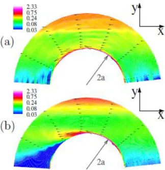
Recently, shear-thickening phenomena have caught more attention (Brown and Jaeger 2014; Mari et al. 2014; Wyart and Cates 2014). Picano et al. (2013) thought shear-thickening can be due to the augmentation of exclude volume of particles. Fluid inertia causes strong microstructure anisotropy that result in the formation of a shadow region with no relative flux of particles. As shown in Fig 2.8, 2a is the least distance between two particles of radius a, the region with vanishing probability to find another particle in relative motion increases at higher Reynolds numbers. This regions act as an increase of the effective volume of particles: the geometrical volume occupied by the particles plus the volume of the region, thus leading to the augmentation of the viscosity (Picano et al. 2013; Fornari et al. 2016).

(31)

15 Fig 2.8 Contour plot of particle pair relative flux, for = 31.5%: a) Re = 0.1, b) Re = 10. (Picano et al. 2013)

Brown and Jaeger (2014) summarized that there are 3 mechanisms for shear-thickening: 1) Hydro-clustering formation of particles (N. J. Wagner and Brady 2009). Above a

critical shear rate, particles stick together transiently by the lubrication forces and can grow into larger clusters (Fig 2.9). The large clusters result in a larger relative viscosity.

2) Order-disorder transition (Hoffman 1974). Following the increase of shear rate, the arrangement of particles changes from ordered layers to a disordered state, thus the viscosity increases.

3) Particle dilatancy (Brown and Jaeger 2012). When particles are sheared, they try to go around each other, but often cannot approach directly, so the packing volume of particles increases (dilates).

Fig 2.9 Instantaneous configurations of transient clusters in the shear thickening regime, observed using fast confocal microscope. Different colors indicate different clusters. Particles outside the large clusters are drawn with smaller size for clarity (Cheng et al. 2011).

(32)

16 In addition, they found that discontinuous shear-thickening may be related to the jamming effect of suspensions.

2.1.3.3 Other effects

Yield stress

Yield stress has mostly been observed at high concentrations (ϕ > 0.5) and at low shear rates (Dabak and Yucel 1987; Dzuy and Boger 1983; Heymann, Peukert, and Aksel 2002; Hoffman 1992; Jomha et al. 1991; Zhu and Kee 2002). Although the concept of yield stress and its experimental measurement has been a matter of debates (Barnes 1999; Heymann, Peukert, and Aksel 2002; Moller et al. 2009; Nguyen and Boger 1992), most works acknowledged the existence of yield stress in fluids. One focal point of the argument is how to clarify and measure the yield stress experimentally. An apparent yield stress can be observed in a suspension that means the viscosity tends toward infinity at very small shear rates, or there is a finite shear stress without deformation over long experimental time scales (Moller et al. 2009).

Effect of size distribution

As demonstrated in many experimental or simulation studies of bi-dispersed or poly-dispersed suspensions, at the same particle packing fraction, the bi-poly-dispersed or poly- dispersed suspension has a lower viscosity (Chingyi Chang 1994; D’Haene and Mewis 1994; Qi and Tanner 2011; Spangenberg et al. 2014). One widely accepted explanation is the increase of effective maximum volume fraction ϕm-eff. Since small particles may

occupy the space between larger particles, a higher effective packing fraction can be achieved (Metzner 1985). Then, according to equation (2.10), when ϕm-eff increases, the

viscosity decreases. To understand this physically, the small particles can act as lubricants for the flow of the larger particles, thereby reducing the overall viscosity (Servais, Jones, and Roberts 2002).

In addition, ϕm-eff not only depends on the number of discrete size bands (mono-, bi-, tri-,

tetra-dispersed, etc.), but also depends on the size ratio of the diameter of large particles ( ) to that of the smaller ones ( ) in the next particle class ) . For a given particle size distribution, ϕm-eff increases with increasing , and reaches a maximum value at infinite diameter ratio, which can be considered as a mono-dispersed suspension.

Models of maximum volume fraction versus particle size distribution can been found in many articles (Chang and Powell 1994; Chong, Christiansen, and Baer 1971; Shapiro and Probstein 1992; Dörr, Sadiki, and Mehdizadeh 2013; Ouchiyama and Tanaka 1981; Zou

(33)

17 et al. 2003; Farris 1968; Qi and Tanner 2011). Their results confirm the trend described above.

Effect of particle shape

When the particles are non-spherical, there is an extra energy dissipation when the suspension is under flow, which result in an increase of viscosity (Genovese 2012), and its contribution to suspension viscosity depends on the orientation of non-spherical particles. The use of arbitrary shape particles will change the maximum packing fraction and the intrinsic viscosity value (Equation (2.8)). Therefore, to determine the viscosities of non-spherical particle suspensions is to determine their effective maximum packing fraction and the changed intrinsic viscosity value. Generally, particle non-sphericity induces an increase of the intrinsic viscosity value B and a decrease of the effective maximum packing fraction ϕm-eff . But their products remain ≈ 2 (Barnes, Hutton, and

Walters 1989).

For example, Kitano et al. (1981) measured the viscosity of non-spherical particle suspensions. They used equation (2.10) to describe the viscosity of non-spherical particle suspensions. They found that the maximum packing fraction decreased with the increasing of the length ( ) to diameter ( ) ratio ( ). When (spheres), ϕm-eff = 0.68, when (crystals), ϕm-eff =0.44. The same tendency was found by

Mueller et al. (2010), by measuring the viscosity of mono-dispersed prolate and oblate particle suspension.

Effect of particle deformability and particle aggregation : the case of

blood

When particles are deformable, they can alter their shape when stresses are applied (shear stress, collision etc.). Then, they can squeeze each other in the flow of high particle concentration. By these effects, the maximum packing fraction of deformable particle suspension is bigger than that of hard-sphere suspension. According to equation (2.10), the viscosity is thus smaller. Studies about the influence of particle deformability can be found in the articles of Frith and lips (1995), Snabre and Mills (1999). Both their analysis are implemented by considering the change of maximum packing fraction and intrinsic viscosity based on equation (2.8).

One example of deformable particle suspension is blood (Baskurt and Meiselman 2003). Red blood cells are suspended in blood plasma (a Newtonian fluid), with a concentration about 45% in volume. RBCs contain a viscous liquid and are enclosed by a visco-elastic membrane, thus they are highly deformable(Zhang, Johnson, and Popel 2007). With such a structure, RBCs are able to get through the micro-capillary with a diameter of around 4

(34)

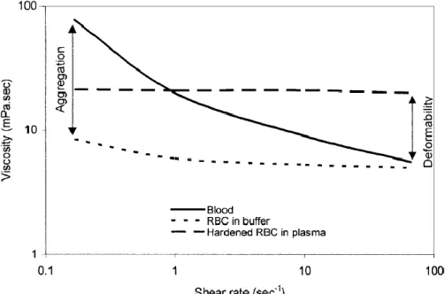
18 µm (Popel and Johnson 2005; Xu, Tian, and Deng 2012). The influence of RBCs deformability on the blood viscosity can be seen in Fig 2.10.

Fig 2.10 Variations of blood viscosity under different conditions as a function of shear rate (Chien 1970)

Due to the deformability of RBCs, the viscosity of blood is much smaller than hardened red blood cells in plasma at shear rates varying from 1s-1_{to 100s}-1_.

Fig 2.11 Rouleaux of human red cells photographed on a microscope slide showing single linear and branched aggregates (left part) and a network (right part). The number of cells in linear array are 2, 4, 9, 15, and 36 in a, b, c, d, f, respectively (Fung 1993).

Other than the deformability of RBCs, the aggregation of red blood cell can also influence the viscosity of blood. As shown in the Fig 2.10, the viscosity of the real blood is much higher than RBCs in buffer at low shear rate (<1s-1_{). RBC aggregation causes a large}

(35)

19 increase in viscosity at low shear rates. When shear rate is near zero, RBCs aggregate to form a big cluster, which then behave like a solid (Fig 2.11).

As the shear rate increases, RBCs aggregates tend to break up into small unit called rouleaux. As the shear rate continues to increase, the average number of RBCs in each rouleaux decreases. If the shear rate is larger than a certain critical value, the rouleaux breaks up into individual cells (Yilmaz and Gundogdu 2008). RBCs tend to aggregate at low shear rates, but when they are in buffer, they do not aggregate. Researchers have proven that the presence of fibrinogen, dextran and globulin proteins in plasma cause the aggregation of RBCs (Fung 1993; C. Wagner, Steffen, and Svetina 2013). According to Yilmaz and Gundogdu (2008), the mechanisms of RBC aggregation can be explained as a balance of aggregation and disaggregation force. Disaggregation forces mainly consist of shear force, repulsive force, and elastic energy of RBC membrane. However, the mechanism of aggregation force is still unclear. There are mainly two models to explain the mechanism of aggregation force based either on bridging or depletion (Wagner et al. 2013).

In a clinical view, studying RBC aggregation is of particular relevance. Quoting Baskurt and Meiselman (2010), “RBCs aggregation should not only be considered as a factor influencing vascular control mechanisms that regulate the distribution of blood flow to various organs and tissues, but should also be considered, more generally, as a phenomenon that interferes with endothelial function and vascular health”. RBC aggregation and its interaction with the surrounding vascular endothelium is now also considered as the central factor to some important vascular functions, such as the regulation of hemostasis, inflammatory response, angiogenesis and vasomotor control. In addition, RBCs aggregates can form large clot, which might completely stop the blood flow. Clot formation is an advantage for wound healing, but in a healthy vessel it might lead to a stroke (thrombus), which is the main cause of death in the developed countries (C. Wagner, Steffen, and Svetina 2013).

The complexity of the in vivo process and studies justifies to split these research works in several simplified problems one of these then concerning the interactions of RBCs and RBC aggregates like in the present work.

Several studies about RBC behaviors in vivo or in vitro have been reviewed such as for microcirculation (Cristini and Kassab 2005; Roman et al. 2013), for venous (Bishop et al. 2001) and for general studies (Baskurt and Meiselman 2003; Baskurt and Meiselman 2010; Rampling et al. 2004; Popel and Johnson 2005). Since it is difficult to produce micro-deformable particles and to do experiments using real blood (for instance, because of visibility isuues in optical measurement technique), many studies about

(36)

20 suspension of deformable particles were performed numerically (Dupin et al. 2007; Bagchi 2007; Zhang, Johnson, and Popel 2008; Juan, Bing, and Hui-Li 2009). However, it is difficult to simulate blood flow with a large quantity of RBCs.

2.2 Flow geometries

2.2.1 Introduction

For the study of the suspension fluid dynamic, a well-defined flow geometry can facilitate the interpretation of data and allow for a mapping of the observed flow dynamics to the rheological properties of the system (Isa et al. 2010). General used flow geometries can be divided into two groups: drag flow geometries like sliding parallel shear plates, in which shear is produced by the relative movements of the two plates, and pressure driven flow geometries, in which shear is generated by the pressure difference over a closed conduit.

2.2.2 Drag flow geometries

2.2.2.1 Parallel shear plates

Parallel shear plates are implemented simply by placing the fluid between two parallel plates which are much larger than their separation . The motions of the fluid are induced by the movements of the plates (Fig 2.11). However, due to their construction, they can only achieve finite strains after which the direction of motion must be reversed. Thus, they are particularly suited for oscillatory strain studies (Isa et al. 2010).

Fig 2.11 Schematic illustration of parallel shear plates

(2.11)

For a Newtonian fluid without slip and sufficiently far from the edges, the induced flow velocity can be expressed as equation (2.11), where is the distance between the two plates, and are the velocity of the top and the bottom plates respectively.