HAL Id: tel-01265957
https://hal.archives-ouvertes.fr/tel-01265957v2
Submitted on 23 Sep 2016HAL is a multi-disciplinary open access archive for the deposit and dissemination of sci-entific research documents, whether they are pub-lished or not. The documents may come from teaching and research institutions in France or abroad, or from public or private research centers.
L’archive ouverte pluridisciplinaire HAL, est destinée au dépôt et à la diffusion de documents scientifiques de niveau recherche, publiés ou non, émanant des établissements d’enseignement et de recherche français ou étrangers, des laboratoires publics ou privés.
Antoine Cully
To cite this version:
Antoine Cully. Creative Adaptation through Learning. Artificial Intelligence [cs.AI]. Université Pierre et Marie Curie - Paris VI, 2015. English. �NNT : 2015PA066664�. �tel-01265957v2�
Spécialité : Informatique (EDITE) Présentée par : M. Antoine Cully
Soutenue le : 21 Décembre 2015 Pour obtenir le grade de
Docteur de l’Université Pierre et Marie Curie
Creative Adaptation through
Learning
Rapporteurs Marc Schoenauer - INRIA Saclay - Île-de-France David Filliat - ENSTA - ParisTech
Examinateurs Raja Chatila - Univ. Pierre et Marie Curie - ISIR Jan Peters - Technische Universität Darmstadt
Jonas Buchli - ETH Zurich
Invitée Eva Cruck - Direction Générale de l’Armement
Agence Nationale de la Recherche Directeur Stéphane Doncieux - Univ. Pierre et Marie Curie - ISIR Co-encadrant Jean-Baptiste Mouret - Univ. Pierre et Marie Curie - ISIR
Les robots ont profondément transformé l’industrie manufacturière et sont suscepti-bles de délivrer de grands bénéfices pour la société, par exemple en intervenant sur des lieux de catastrophes naturelles, lors de secours à la personne ou dans le cadre de la santé et des transports. Ce sont aussi des outils précieux pour la recherche scientifique, comme pour l’exploration des planètes ou des fonds marins. L’un des obstacles majeurs à leur utilisation en dehors des environnements parfaitement contrôlés des usines ou des laboratoires, est leur fragilité. Alors que les animaux peuvent rapidement s’adapter à des blessures, les robots actuels ont des difficultés à faire preuve de créativité lorsqu’ils doivent surmonter un problème inattendu: ils sont limités aux capteurs qu’ils embarquent et ne peuvent diagnostiquer que les situations qui ont été anticipées par leur concepteurs.
Dans cette thèse, nous proposons une approche différente qui consiste à laisser le robot apprendre de lui-même un comportement palliant la panne. Cependant, les méthodes actuelles d’apprentissage sont lentes même lorsque l’espace de recherche est petit et contraint. Pour surmonter cette limitation et permettre une adaptation rapide et créative, nous combinons la créativité des algorithmes évolutionnistes avec la rapidité des algorithmes de recherche de politique (policy search).
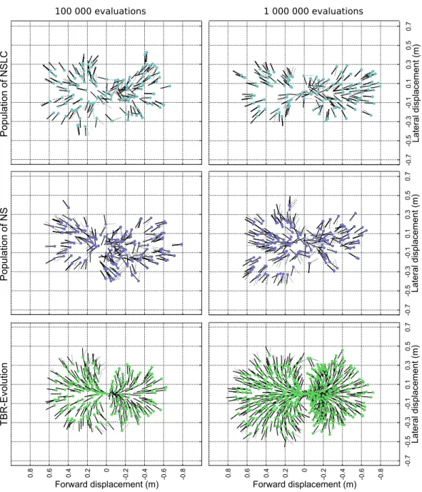
Notre première contribution montre comment les algorithmes évolutionnistes peuvent être utilisés afin de trouver, non pas une solution, mais un large ensemble de solutions à la fois performantes et diverses. Nous appelons ces ensembles de solutions des répertoires comportementaux (behavioral repertoires). En découvrant de manière autonome ces répertoires comportementaux, notre robot hexapode a été capable d’apprendre à marcher dans toutes les directions et de trouver des milliers de façons différentes de marcher. A notre sens, ces répertoires comportementaux capturent la créativité des algorithmes évolutionnistes.
La seconde contribution que nous présentons dans ce manuscrit combine ces répertoires comportementaux avec de l’optimisation Bayesienne. Le répertoire com-portemental guide l’algorithme d’optimisation afin de permettre au robot endom-magé de réaliser des tests intelligents pour trouver rapidement un comportement de compensation qui fonctionne en dépit de la panne. Nos expériences démontrent que le robot est capable de s’adapter à la situation moins de deux minutes malgré l’utilisation d’un grand espace de recherche et l’absence de plan de secours préétab-lis. L’algorithme a été testé sur un robot hexapode endommagé de 5 manières différentes, comprenant des pattes cassées, déconnectées ou arrachées, ainsi que sur un bras robotisé avec des articulations endommagées de 14 façons différentes.
Pour finir, notre dernière contribution étend cet algorithme d’adaptation afin de pallier trois difficultés qui sont couramment rencontrées en robotique: (1) per-mettre de transférer les connaissances acquises sur une tâche afin d’apprendre plus rapidement à réaliser les tâches suivantes, (2) être robuste aux solutions qui ne peuvent pas être évaluées sur le robot (pour des raisons de sécurité par exemple), et
qui sont susceptibles de pénaliser les performances d’apprentissage et (3) adapter les informations reçues a priori par le robot, qui peuvent être trompeuses, afin de maximiser leur utilité. Avec ces nouvelles propriétés, notre algorithme d’adaptation a permis à un bras robotisé endommagé d’atteindre successivement 20 cibles en moins de 10 minutes en utilisant uniquement les images provenant d’une caméra placée à une position arbitraire et inconnue du robot.
A travers l’ensemble de cette thèse, nous avons mis un point d’honneur à con-cevoir des algorithmes qui fonctionnent non seulement en simulation, mais aussi en réalité. C’est pourquoi l’ensemble des contributions présentées dans ce manuscrit ont été testées sur au moins un robot physique, ce qui représente l’un des plus grands défis de cette thèse. D’une manière générale, ces travaux visent à apporter les fondations algorithmiques permettant aux robots physiques d’être plus robustes, performants et autonomes.
Robots have transformed many industries, most notably manufacturing, and have the power to deliver tremendous benefits to society, for example in search and rescue, disaster response, health care, and transportation. They are also invaluable tools for scientific exploration of distant planets or deep oceans. A major obstacle to their widespread adoption in more complex environments and outside of factories is their fragility. While animals can quickly adapt to injuries, current robots cannot “think outside the box” to find a compensatory behavior when they are damaged: they are limited to their pre-specified self-sensing abilities, which can diagnose only anticipated failure modes and strongly increase the overall complexity of the robot. In this thesis, we propose a different approach that considers having robots learn appropriate behaviors in response to damage. However, current learning techniques are slow even with small, constrained search spaces. To allow fast and creative adaptation, we combine the creativity of evolutionary algorithms with the learning speed of policy search algorithms.
In our first contribution, we show how evolutionary algorithms can be used to find, not only one solution, but a set of both high-performing and diverse solutions. We call these sets of solutions behavioral repertoires and we used them to allow a legged robot to learn to walk in every direction and to find several thousands ways to walk. In a sense, these repertoires capture a portion of the creativity of evolutionary algorithms.
In our second contribution, we designed an algorithm that combines these be-havioral repertoires with Bayesian Optimization, a policy search algorithm. The repertoires guide the learning algorithm to allow damaged robots to conduct in-telligent experiments to rapidly discover a compensatory behavior that works in spite of the damage. Experiments reveal successful adaptation in less than two minutes in large search spaces and without requiring self-diagnosis or pre-specified contingency plans. The algorithm has been tested on a legged robot injured in five different ways, including damaged, broken, and missing legs, and on a robotic arm with joints broken in 14 different ways.
Finally, in our last contribution, we extended this algorithm to address three common issues in robotics: (1) transferring knowledge from one task to faster learn the following ones, (2) dealing with solutions that cannot be evaluated on the robot, which may hurt learning algorithms and (3) adapting prior information that may be misleading, in order to maximize their potential utility. All these additional features allow our damaged robotic arm to reach in less than 10 minutes 20 targets by using images provided by a camera placed at an arbitrary and unknown location. Throughout this thesis, we made a point of designing algorithms that work not only in simulation but also in reality. Therefore, all the contributions presented in this manuscript have been evaluated on at least one physical robot, which represents one of the biggest challenges addressed in this thesis. Globally, this work aims to provide the algorithmic foundations that will allow physical robots to be more robust, effective and autonomous.
A PhD thesis is quite an adventure and even if there is a main character, it is, in fact, teamwork. With these few lines, I would like to warmly thank all my team-mates for their help and their support that allowed me to enjoy this intense journey. Like in every journey, some moments have been more difficult than others. Fortunately, my dear Coralie was always present to cheer me on during time of doubt. She has also been extremely patient during the long evenings and nights that I spent to finish a paper, an experiment or simply to find a bug in my code. She has been my highest support during all these 3 years and the manuscript that you are currently reading would not have been the same without her.
It goes without saying that this thesis would also not have been the same without my supervisor Jean-Baptiste Mouret. He taught me everything I know in computer science and in scientific research in general. He believed in me and gave me enough freedom to explore my own ideas, while keeping a close eye on my pro-gresses to prevent me to go on bad paths. He made me face challenges that I never expected to be able to accomplish. The current young scientist that I am today is undoubtedly the fruit of his supervision and I am proud of being one of his students. The quality of supervision that I had during my thesis is also highly due to Stéphane Doncieux, who gave us the means and freedom to investigate our ideas within a fantastic working environment that we name AMAC team. His pieces of advice have always been extremely valuable and I really enjoyed our fruitful discussions about dreams in robotics.
Within the AMAC team and the ISIR laboratory in general, I had the luck to be in an excellent working environment that both stimulated and encouraged me. In addition to the environment, I had outstanding colleagues. The researchers of the team have always been here to share their own experience, to ask questions or to give pieces of advice. They are the heart of this big family that allows young PhD-students to grow up and I wish to be able, at one point, to help, support, and to advise young students as they did with me.
In particular, I would like to thank the marvelous members of the “famous J01” and affiliates (the list is too large, but they will recognise themselves). Several generations of PhD-students passed, but always with a lot of laughs, jokes and pranks. In addition to be my colleagues, most of them are today my friends.
The only regret that I have about this thesis is that, at the end, I have to leave this exceptional team.
A good preparation is required before every adventure, and for my prepa-ration before the PhD-Thesis, I would like to thank all my teachers from the Polytech’Paris-UPMC engineer school (who are, for most of them, also my colleagues in the ISIR lab). In addition to teach me their knowledge, they also exchange with me their passion about robotics and the profession of researcher. Even if they do not fully understood what I was doing, I would like to thank my family, who has always encouraged me to follow my desires and gave me the means to accomplish them.
I would like to thank the members of the jury of my PhD defense for accepting to be part of the jury. Their final judgement will validate the fruit of three intense and fascinating years of work and symbolize the end of this fabulous adventure.
Finally, I would like also to thank the DGA and the University Pierre and Marie Curie, who gave me the opportunity to do this fantastic journey.
1 Introduction 1 2 Background 7 2.1 Introduction. . . 7 2.2 Evolutionary algorithms . . . 10 2.2.1 Principle . . . 10 2.2.2 Multi-objective optimization . . . 15 2.2.3 Novelty Search . . . 18 2.2.4 Evolutionary robotics . . . 20
2.2.5 The Reality Gap problem and the Transferability approach . 22 2.2.6 Partial conclusion . . . 23
2.3 Policy search algorithms . . . 24
2.3.1 Common principles . . . 24
2.3.2 Application in behavior learning in robotics . . . 33
2.3.3 Partial conclusion . . . 34
2.4 Bayesian Optimization . . . 35
2.4.1 Principle . . . 35
2.4.2 Gaussian Processes . . . 35
2.4.3 Acquisition function . . . 42
2.4.4 Application in behavior learning in robotics . . . 44
2.4.5 Partial conclusion . . . 46
2.5 Conclusion . . . 47
3 Behavioral Repertoire 49 3.1 Introduction. . . 50
3.1.1 Evolving Walking Controllers . . . 50
3.1.2 Evolving behavioral repertoires . . . 52
3.2 The TBR-Evolution algorithm . . . 54
3.2.1 Principle . . . 54
3.2.2 Experimental validation . . . 58
3.3 The MAP-Elites algorithm . . . 76
3.3.1 Principle . . . 76
3.3.2 Experimental validation . . . 80
3.4 Conclusion . . . 87
4 Damage Recovery 89 4.1 Introduction. . . 90
4.1.1 Learning for resilience . . . 91
4.1.2 Resilience with a self-model . . . 92 4.1.3 Dealing with imperfect simulators to make robots more robust 95
4.2 The T-Resilience algorithm . . . 97
4.2.1 Motivations and principle . . . 97
4.2.2 Method description. . . 97
4.2.3 Experimental validation . . . 99
4.2.4 Results . . . 104
4.2.5 Partial conclusion . . . 109
4.3 The Intelligent Trial and Error algorithm . . . 109
4.3.1 Motivations and principle . . . 109
4.3.2 Method description. . . 112
4.3.3 Experimental validation . . . 115
4.3.4 Partial conclusion . . . 139
4.4 Conclusion . . . 140
5 Knowledge Transfer, Missing Data, and Misleading Priors 143 5.1 Introduction. . . 144
5.2 Knowledge Transfer . . . 145
5.2.1 Motivations . . . 145
5.2.2 Principle . . . 146
5.2.3 Method Description . . . 148
5.2.4 Multi-Channels Regression with Bayesian Optimization . . . 151
5.2.5 Experimental Validation . . . 157 5.3 Missing Data . . . 165 5.3.1 Motivations . . . 165 5.3.2 Principle . . . 165 5.3.3 Method Description . . . 167 5.3.4 Experimental Validation . . . 169 5.4 Misleading Priors . . . 172 5.4.1 Motivations . . . 172 5.4.2 Principle . . . 173 5.4.3 Method Description . . . 173 5.4.4 Experimental Validation . . . 175
5.5 Evaluation on the physical robot . . . 180
5.5.1 The whole framework . . . 180
5.5.2 Experimental setup. . . 181
5.5.3 Experimental Results . . . 184
5.6 Conclusion . . . 184
6 Discussion 187 6.1 Using simulations to learn faster . . . 188
6.2 Gathering collections of solution into Behavioral Repertoires. . . 190
6.3 Exploring the information provided by Behavioral Repertoires. . . . 193
Bibliography 199
A The Hexapod Experiments 227
A.1 The Hexapod Robot . . . 227
A.2 The Hexapod Genotypes and Controllers. . . 227
A.2.1 The first version (24 parameters) . . . 227
A.2.2 The second version (36 parameters) . . . 229
B The Robotic Arm experiments 231 B.1 The Robotic Arm: First setup . . . 231
B.2 The Robotic Arm: Second setup . . . 232
B.3 The Arm Controller . . . 233
C Parameters values used in the experiments 235 C.1 TBR-Evolution experiments . . . 235
C.2 T-Resilience experiments. . . 236
C.3 Intelligent Trial and Error experiments . . . 236
C.3.1 Experiments with the hexapod robot . . . 236
C.3.2 Experiments with the robotic arm . . . 236
C.4 State-Based BO with Transfer, Priors and blacklists . . . 237
D Other 239 D.1 Appendix for the T-resilience experiments . . . 239
D.1.1 Implementation details for reference experiments . . . 239
D.1.2 Validation of the implementations . . . 242
D.1.3 Median durations and number of tests . . . 244
D.1.4 Statistical tests . . . 244
D.2 Methods for the Intelligent Trial and Error algorithm and experiments245 D.2.1 Notations . . . 245
D.2.2 Hexapod Experiment. . . 245
D.2.3 Robotic Arm Experiment . . . 248
D.2.4 Selection of parameters . . . 249
D.2.5 Running time . . . 251
D.3 Notation for the State-Based BO with Transfer, Priors and blacklists algorithms . . . 253
Introduction
In 1950, Alan Turing proposed to address the question “can machines think?” via an “imitation game”, which aims to assess machines’ ability to exhibit behaviors that are indistinguishable from those of a human (Turing,1950). In practice, this game involves a human (the evaluator) that has to distinguish between a human and a machine by dialoguing with them via a keyboard and a screen interface. The objective of Alan Turing was to substitute the initial question “can machines think?” by “Can a machine communicate in a way that makes it indistinguishable from a human”. This question and this reasoning had, and still has, a strong impact in artificial intelligence (Warwick and Shah,2015;Russell et al.,2010). However, a robot is not only a mind in a computer, it is an agent “that has a physical body” (Pfeifer and Bongard,2007) and “that can be viewed as perceiving its environment through sensors and acting upon that environment through effectors” (Russell et al.,
2010). In order to transpose Turing’s approach into robotics, his question could be considered from a more general point of view: “Can a robot act in a way that makes it indistinguishable from a human?”. Without directly considering humans, we can wonder: can robots act more like animals than like current machines (Brooks,
1990)? But, what is acting like an animal? Put differently, what distinguishes a robot from an animal? In this manuscript, we will consider that one of the most striking differences between animals and robots is the impressive adaptation abilities of animals (Meyer,1996); as a result, we will propose new algorithms to reduce this difference.
After more than 50 years of research in robotics, several breakthroughs have been achieved. For example, a surgeon located in New York operated on a patient in France with a transatlantic robot-assisted telesurgery (Marescaux et al., 2001). The recent advances in 3D printing allowed researchers to automatically design and manufacture robotic lifeforms from their structure to their neural network with an evolutionary algorithm (Lipson and Pollack, 2000). The robots from Boston Dy-namics, like the Bigdog (which is robust to uneven terrains, Raibert et al.(2008)), the Cheetah (which runs at 29 mph (46 km/h)) and Atlas (which is an agile an-thropomorphic robot) or the Asimo robot from Honda are good examples of very sophisticated systems that show impressive abilities. These noticeable advances suggest that robots are promising tools that can provide large benefits to the so-ciety. For example, we can hope that robots will one day be able to substitute humans in the most dangerous tasks they have to perform, like intervening in nu-clear plants after a disaster (Nagatani et al.,2013) or in search and rescue missions after earthquakes (Murphy, 2004;Murphy et al.,2008).
While a few robots start to leave the well-controlled environments of factories to get in our homes, we can observe that most of them are relatively simple robots. More advanced robots, that is, more versatile robots, have the power to deliver tremendous benefits to society. Nonetheless, a slight increase in versatility typ-ically results in a large increase in the robots’ complexity, which, in turn, makes such versatile robots much more expensive and much more damage-prone than their simpler counterparts (Sanderson, 2010; Carlson and Murphy, 2005). This “expo-nential complexity” is a major obstacle to the widespread adoption of robots in complex environments and for complex missions.
In more concrete terms, the success of robotic vacuum cleaners and lawn mowers mainly stems from the simplicity of their task, which is reflected in the simplicity of the robots: they can perform only two types of action (moving forward/backward or turning); they perceive only one thing (the presence of obstacles); and they react with predefined behaviors to the encountered situations (Brooks et al.,1986;Brooks,
1990). With more complex robots, the situation is more complicated because they involve more complex behaviors and require a deeper understanding of the context. For example, a robot in a search and rescue mission (Murphy et al.,2008) has to deal with uneven terrains and to locate injured people. In order to be effective, it will have to move obstacles, to repatriate victims and to cooperate with other robots. With all these tasks, these robots may face an almost infinite number of situations, like different types of terrains, different types of disasters or different types of injured people. In other words, while it is possible to foresee most of the situations a simple robot (like a vacuum cleaner) may face, it is unfeasible to predefine how complex robots have to react in front of the quasi infinite set of situations they may encounter, unless having a team of engineers behind each robot1.
In addition, the high complexity of versatile robots is bound to increase their fragility: each additional actuator or sensor is potentially a different way for a robot to become damaged. For example, many robots sent in search and rescue missions have been damaged and unable to complete their mission. In 2005, two robots were sent to search for victims after a mudslide near Los Angeles (La Conchita). Unfortunately, they became unable to continue their missions after only two and four minutes because of a root in the wet soil and a thick carpet in a house (Murphy et al., 2008). Similarly, after a mine explosion in West Virginia (Sago in 2006): the robot sent to find the victims became stuck on the mine rails after only 700 meters (Murphy et al.,2008). Five years later, the same kind of scenario repeated several times after the nuclear accident at the Fukushima nuclear power plants that happened in 2011. For example, one robot has been lost in 2011 because its communication cable got snagged by the piping of the plant (Nagatani et al.,2013) and a second robot has been lost in 2015 after a fallen object blocked its path. In all these examples, the robots have been abandoned and the missions aborted, which
1For example, teams of engineers are involved in the control-loops (DeDonato et al., 2015) of
robots that participate to the DARPA Robotics Challenge (Pratt and Manzo,2013) in order to
can lead to dramatic consequences when lives are at stake.
The question of fault tolerance is a classic topic in engineering, as it is a common problem in aviation and aerospace systems. Current damage recovery in deployed systems typically involves two phases: (1) performing self-diagnosis thanks to the embedded sensors and then (2) plan or select the best contingency plan according to the diagnosis (Kluger and Lovell,2006;Visinsky et al.,1994;Koren and Krishna,
2007). The side effect of this kind of approach is that it requires anticipating all the damage conditions that may occur during the robot’s mission. Indeed, each type of damage that should be diagnosed requires having the proper sensor at the right place, similarly to a doctor who uses different tools to diagnose different diseases, electrocardiogram to detect heart diseases and MRI for cancer cells. As a consequence, the robot’s abilities to diagnose a damage condition directly depend on its embedded sensors. As the robots and their missions increase in complexity, it becomes almost unfeasible to foresee all the damage conditions that may occur and to design the corresponding diagnostic modules and contingency plans. This is the beginning of a vicious circle that prevents us from keeping the costs reasonable, as each of these modules can be damaged too and may thus require additional sensors. Animals, and probably humans, respond differently when they face an unex-pected situation or when they are injured (Jarvis et al.,2013; Fuchs et al., 2014): they discover by trial and error a new behavior. For example, when a child has a sprain ankle, he is able to discover, without the diagnosis of a doctor, that limping minimizes pain and allows him to go back home.
The objective of the algorithmic foundations presented in this manuscript is to allow robots to do the same: making robots able to learn on their own how to deal with the different situations they may encounter. With improved learning abili-ties, robots will become able to autonomously discover new behaviors in order to achieve their mission or to cope with a damage. The overall goal of this promising approach is to help develop more robust, effective, autonomous robots by removing the requirement for engineers to anticipate all the situations that robots may en-counter. It could, for example, enable the creation of robots that can help rescuers without requiring their continuous attention, or making easier the creation of per-sonal robotic assistants that can continue to be helpful even when a part is broken. Throughout this manuscript, we will mainly consider the challenge of damage re-covery, though adapting to other unforeseen situations that do not involve damage would be a natural extension of this work.
In order to effectively discover new behaviors, learning processes have to be both fast and creative. Being able to learn quickly (in terms of both time and number of evaluations) new behaviors is critical in many situations. The first reason is that most autonomous robots run on batteries, and as a consequence, it is likely that a robot that spends too much time learning new behaviors will run out of battery before achieving its mission. The second reason is that many situations require reacting quickly, typically after a disaster. Therefore, we cannot have robots wasting hours trying to learn new behaviors when people’s lives are in danger. Creativity, which “ involves the production of novel, useful [solutions]” (Mumford,
2003), is an important property for learning algorithms, as it influences the number of situations in which systems are able to find appropriate solutions. This property requires algorithms to explore large search spaces to discover behaviors that are different from what they already know (Lehman and Stanley, 2011a). Transposed to robotics, the creativity of the algorithm determines the number of unforeseen situations that the robot can handle. For example, riding a bicycle is different from walking or limping. To allow a robot to adapt to a large variety of situations, a learning algorithm has to be able to find all these different types of behaviors, regardless the initial or current behavior of the robot.
Unfortunately, speed and creativity are most of the time antagonistic properties of learning algorithms because exploring a large search space, that is, searching for creative solutions, requires a large amount of time. In the next chapter (chapter2), we review the different families of learning algorithms and compare their creativity and learning speed. We focus our review on evolutionary algorithms (Eiben and Smith, 2003) and Policy Search methods (Kober et al., 2013) because they are the main families of algorithms used to learn low-level behaviors (motor skills) in robotics.
In chapter 3, we present how the creativity of evolutionary algorithms can be employed to discover large collections of behaviors. For example, we show how a legged robot can autonomously discover several hundred behaviors that allow it to walk in every direction. In other experiments, the same robot also discovered several thousand ways of walking in a straight line. We call these large collections of behaviors Behavioral Repertoires.
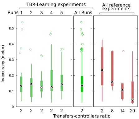
In the chapter 4, we apply learning algorithms for on-line damage recovery. One of the main challenges is to reduce the required time to adapt while keeping the search space as open as possible to be able to deal with a large variety of situations. In the first part of this chapter, we show how combining simulations and physical experiments allows the algorithm to transfer the majority of the search space exploration in simulation. In the second part of this chapter, we highlight how behavioral repertoires, introduced in the previous chapter, can be combined with a policy search algorithm to guide the exploration process. With these two principles, we propose an algorithm that couples the creativity of evolutionary algorithm and the speed of policy search algorithms to allow damaged robots to conduct intelligent experiments to rapidly discover compensatory behaviors that work in spite of the damage situations. For example, our experiments show a hexapod robot and a robotic arm that recover from many damage conditions in less than 2 minutes, that is, much faster than the state of the art.
The last chapter (chapter5) extends our damage recovery algorithm to deal with 3 issues that frequently impact robotic experiments: (1) transferring knowledge from one task to learn the following ones faster, (2) dealing with solutions that cannot be evaluated on the robot, which may hurt learning algorithms and (3) adapting prior information that may be misleading, in order to maximize their potential utility. With these extensions, our algorithm aims to become a generic framework that can be used with a large variety of robots to learn and adapt in
numerous situations.
Before the conclusion of this manuscript, we discuss the current limitations of our methods and the different approaches that we plan to investigate in order to circumvent them. In this last chapter (chapter 6), we also highlight the links that may exist between our methods and observations made in neuroscience.
Background
Contents 2.1 Introduction . . . . 7 2.2 Evolutionary algorithms . . . . 10 2.2.1 Principle . . . 10 2.2.2 Multi-objective optimization . . . 15 2.2.3 Novelty Search . . . 18 2.2.4 Evolutionary robotics . . . 202.2.5 The Reality Gap problem and the Transferability approach . 22 2.2.6 Partial conclusion . . . 23
2.3 Policy search algorithms . . . . 24
2.3.1 Common principles . . . 24
2.3.2 Application in behavior learning in robotics . . . 33
2.3.3 Partial conclusion . . . 34
2.4 Bayesian Optimization . . . . 35
2.4.1 Principle . . . 35
2.4.2 Gaussian Processes . . . 35
2.4.3 Acquisition function . . . 42
2.4.4 Application in behavior learning in robotics . . . 44
2.4.5 Partial conclusion . . . 46
2.5 Conclusion . . . . 47
2.1
Introduction
Learning algorithms aim to provide systems with the ability to acquire knowledge and skills to solve a task without being explicitly programmed with a solution. For example,Mitchell(1997) proposed this definition: “The field of machine learning is concerned with the question of how to construct computer programs that automati-cally improve with experience.” Learning algorithms are traditionally divided into three categories of algorithms depending on the quantity of knowledge about the solutions that is provided to the system (Haykin,1998;Russell et al.,2010): (1) In supervised learning, a “teacher” provides to the system a error signal that reflects the difference between the output value and the expected value. These algorithms
are typically applied on classification problems in which the system has a database of inputs examples and corresponding outputs that the system should reproduce. Based on these examples the goal of the algorithm is to learn a generalization of these examples to deal with unknown examples. Conversely, (2) in unsupervised learning (Hastie et al.,2009), there is no “teacher” and the system has no informa-tion about the consequences (or outputs) of its choices. Consequently, the system has to find hidden structures in the obtained data in order to distinguish them. Clustering algorithms (Xu et al., 2005) are a good example of unsupervised learn-ing algorithms. They use the spatial distribution of the data to infer clusters that are likely to correspond to different classes. (3) Reinforcement Learning algorithms (Kober et al.,2013) are in a way situated in between these two families of algorithms. While the correct inputs/outputs pairs are never presented, the “teacher” provides a qualitative feedback after the system has performed a sequence of actions. Most of the time, this feedback is less informative than in supervised learning algorithms. It can be for example a reward value, which does not indicate the actual solution but rather states if the performed action is better or not than the previous ones.
More recently, several other families of learning algorithms have emerged and do not fit well in these three categories. For example, intrinsically motivated learn-ing (Oudeyer et al.,2007;Baldassarre and Mirolli,2013;Delarboulas et al.,2010), in which the system defines on his own the value of its actions, can be considered as both an unsupervised learning algorithm because there is no teacher, and as a reinforcement learning algorithm because the system tries to maximize the feed-back provided by its internal motivation modules. Another example of a recent approach that does not fit in these categories is Transfer learning (Pan and Yang,
2010;Thrun,1996). This approach consists in transferring knowledge acquired on previous tasks to new ones. It consequently shares similarities with both super-vised and unsupersuper-vised learning algorithms, as the former task is most of the time learned thanks to a “teacher”, while the links with the following tasks have to be au-tonomously inferred by the system. Imitation learning (Billard et al.,2008;Schaal,
1999) is another family of algorithms that can be situated on the borderlines of the traditional classifications. In this case, the system aims to reproduce a movement showed by a “teacher”, for example via kinesthetic teaching. This technique shares similarities with supervised learning algorithms, as there is a “teacher” showing the solution. However, the link between the recorded data and the corresponding motor commands is unknown and the robot has to learn to reproduce the movement by minimizing a cost value, like in reinforcement learning, which corresponds to the differences between the taught movement and the robot’s behavior.
Learning a behavior in an unforeseen situation, like after mechanical damage, is typically a reinforcement learning problem, because the robot has to get back its initial performance and no “teacher” can provide examples of good solutions. The robot has to learn on its own how to behave in order to maximize its performance by using its remaining abilities.
The definition of reinforcement learning (RL) from Sutton and Barto (1998a) states that: “Reinforcement learning is learning what to do so as to maximize a
numerical reward signal. The learner is not told which actions to take, as in most forms of machine learning, but instead must discover which actions yield the most reward by trying them.” In other words, a RL algorithms aims to solve a task formulated as a cost function that has to be minimized or as a reward (also called quality or performance) function that has to be maximized. Based on this function (for instance named f ), we can define a reinforcement learning algorithm as an algorithm that solves this equation (considering f as a reward function):
x∗ = arg max
x
f (x) (2.1)
The goal of the algorithm is thus to find the politic or behavior x∗ that maximizes the reward function (Sutton and Barto,1998a;Russell et al.,2010).
We can see here that a RL problem can be formulated as a standard optimiza-tion problem. However, when learning a behavior, the optimized funcoptimiza-tion as well as its properties and gradient are typically unknown. A typical example is a legged robot learning to walk: it has to learn how to move its legs in order to keep balance and to move. In this context, the reward function can be for example the walking speed and the solutions can be parameters that define leg trajectories or synaptic weights of neural networks that control the motors. The function that maps these parameters to the reward value is unknown. Consequently, in order to acquire infor-mation about this function, the system has to try potential solution and to record its performance. This type of function is called black-box functions and makes impos-sible to use standard optimization algorithms, like linear or quadratic programming (Dantzig, 1998; Papadimitriou and Steiglitz, 1998) or the Newton’s optimization method (Avriel,2003), which require the problem to be linear/quadratic or to have access to the derivative of the function.
Reinforcement learning algorithms have been designed to deal with this kind of function and gather several sub-families of techniques, like Policy Search algorithms (Kober et al.,2013;Deisenroth et al.,2013b) or Differential Dynamic Programming (Bertsekas et al., 1995; Sutton et al., 1992). However, the name reinforcement learning refers most of the time to the first family of RL algorithms that have been proposed, making the distinction between the general RL family and these traditional algorithms sometimes difficult and confusing. These algorithms aim to associate to every state of the robot to a reward (it corresponds to the “value func-tion”) and then use this information to determine the optimal policy to maximize the reward. This family of algorithms is for example composed by the Q-learning algorithm (Watkins, 1989; Watkins and Dayan, 1992), the State-Action-Reward-State-Action algorithm (SARSA, Rummery and Niranjan(1994)) or the Time Dif-ference Learning algorithm (TD-Learning, Sutton and Barto (1998b)). However, the vast majority of these algorithms are designed to work with small state spaces (for example 2D locations in maze experiments,Thrun(1992)) and with discretized state and action spaces (for example discrete actions can be: move up, move down, move right, move left, etc.).
While these traditional reinforcement algorithms are beneficial to learn discrete high-level tasks (like in path-planning problem (Singh et al., 1994), to learn to
play video games (Mnih et al., 2015)); learning low-level behaviors or motor skills in robotics (like walking gaits or reaching movements) involves most of the time using continuous and high dimensional state and action spaces. These aspects contrast with the constraints of traditional RL algorithms and this is why most of applications of RL in robotics use Policy Search algorithms (PS) (Kober et al.,
2013), which are known to have better scalability and to work in continuous domains (Sutton et al.,1999;Deisenroth et al.,2013b).
Another family of algorithms widely used to learn behaviors in robotics are the evolutionary algorithms (EAs, Eiben and Smith(2003)). These algorithms are most of the time considered apart from the general family of reinforcement learning algorithms, because they come from different concepts and ideas. However, we can underline that EAs fit perfectly into the definition of RL algorithms presented above. They are used to optimize a fitness function, which is similar to a cost or a reward function, and they test different potential solutions (gathered in a population) to gather information about this unknown function.
In this chapter, we will present in detail both Evolutionary algorithms and Policy Search algorithms, as they are widely used to learn low-level behaviors in robotics. In the last part of this chapter we provide a concise tutorial on Bayesian Optimiza-tion, a model-based policy search algorithm that is considered as the state-of-the-art in learning behaviors in robotics. The objective of this overview is to get a global picture of the advantages and the limitations of each of these algorithms, which will be useful to design a learning algorithm that will allow robots to adapt to unforeseen situations. We will in particular focus our attention on their ability to find creative solutions and the number of trials on the robot required to find these solutions. The creativity of an algorithm is related to its ability to perform a global optimization and to the size of the search space they can deal with. Such property is important as a behavior that works in spite of a damage may be substantially different from the robot’s initial behaviors. For example, a six-legged robot with a damaged leg will walk differently with its 5 remaining legs than when it was intact. The learning speed of the algorithm is also a very important aspect of learning algorithms as it directly impacts the autonomy of the robot. A robot requiring to test hundreds of behaviors to find a solution is likely to run out of battery or to aggravate its condition.
2.2
Evolutionary algorithms
2.2.1 Principle
Evolutionary Algorithms (EAs) take inspiration from the synthetic theory of evo-lution. This theory, which emerged in the 30’s, combines the Darwinian theory of evolution (Darwin,1859), the Mendelian theory of heredity (Mendel,1865) and the theory of population genetics (Haldane,1932). It details the mechanisms that drive the diversity of individuals among a population and those that allow some traits to be transferred from one individual to another though heredity. The synthetic
the-ory of evolution mainly relies on the idea that the DNA encodes the characteristics of the individual and that each DNA sequence is different. During the reproduc-tion process, several sequences are combined and mutated in order to create new individual, which promote the diversity of individuals in the population.
Evolutionary computation algorithms tend to employ an abstract representation of this theory in order to use the adaptation abilities of natural evolution to a large set of problems. This abstraction stands on 4 principles:
• Diversity of individual: Each individual, even from the same specie, is differ-ent.
• Struggle for life: Every individual cannot survive because the natural re-sources are limited. Consequently, the individuals have to compete to survive. • Natural selection: The individuals survive because they have particular
char-acteristics that make them more adapted.
• Heredity of traits: The surviving individuals share some of their characteristics to their descendants.
EAs are used to solve a large panel of optimization, design and modeling prob-lems (Eiben and Smith,2015). For example, they can generate structures (of neural networks,Stanley and Miikkulainen(2002), or of objects,Hornby et al.(2011); Lip-son and Pollack (2000)), images (Secretan et al., 2008; Sims, 1991), weights of neural networks (Floreano and Mondada,1994;Whitley et al.,1990;Devert et al.,
2008), virtual creatures (Sims, 1994; Lehman and Stanley, 2011b), robotic con-troller (Zykov et al.,2004;Godzik et al.,2003), soft robots (Cheney et al.,2013) or chemistry reactions (Gutierrez et al.,2014;Dinh et al.,2013). It is also very inter-esting to mention that, while the EAs come from the synthetic theory of evolution, EAs are also promising tool to study natural evolution (Smith,1992;Lenski et al.,
1999). For example,Clune et al.(2013) used evolutionary algorithms to investigate the evolutionary origins of modularity in biological networks. In other examples, EAs have also been used to explain the emergence of collaborative behaviors like cooperation (Bernard et al.,2015), altruism (Montanier and Bredeche,2013;Waibel et al.,2011) or communication (Floreano et al.,2007;Mitri et al.,2009;Wischmann et al.,2012).
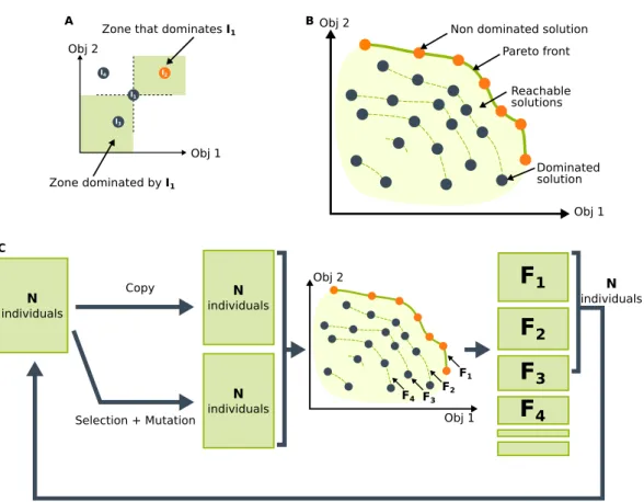
These application examples, while being incomplete, show that the domain of EAs is very large. However, it is interesting to note that most of them rely on the same principles. In general, one iteration of EAs (called generation) involves 3 steps (Eiben and Smith, 2003). After the initialization (typically random) of the population, (1) all the individuals of the population are evaluated on the problem (see Fig. 2.1B) and are then ranked based on their quality (see Fig. 2.1C). (2) the best individuals survive (see Fig. 2.1 E) while the others are likely to perish (see Fig. 2.1D). This selection process mimics the fact that each individual has to compete in order to survive. (3) The surviving individuals are crossed and mutated to create offspring individuals, which are then used to form a new population.
A B C
D E
Figure 2.1: The main steps of evolutionary algorithms. All the population (A) is evaluated on the task (B). Based on the recorded performance of the individuals (fitness score), the population is sorted (C). The individuals that are in the bottom of the ordering are removed from the population (E) while the others are mutated and crossed in order to create a new population (D). This new population is then used to repeat the process, which ends when a performance criterion is reached or when a predefined number of generations has been executed.
This 3-step process then repeats with the new population making it progressively more adapted to the problem the algorithm is solving. The algorithm stops after a particular amount of time (CPU time or number of evaluations) or after the population has converged.
In the vast majority of work, EAs are employed to solve optimization problems and they are typically well tailored to deal with black-box functions (Eiben and Smith,2003). The particularity of such functions is that no information about the structure or gradient of the function is available. The algorithm can only supply a potential solution and gets the corresponding value, making the optimization prob-lem notably difficult. In EAs, the optimized function is called the fitness function (Eiben and Smith,2003):
Definition 1 (Fitness function) The fitness function represents the require-ments the individuals have to adapt to. Mathematically, it is a function that takes as an input a potential solution (also called an individual) and outputs a fitness score that represents the quality of the individual on the considered problem.
The fitness score of an individual can be seen, from a biological point of view, as its ability to survive in its environment. As describe below, this score has an impact on the selection and reproduction processes. The potential solutions are described thanks to a genotype that can be expanded into a phenotype.
Definition 2 (Genotype and Phenotype) The genotype encodes the informa-tion that characterizes the individual. The phenotype is the expression of the infor-mation contained in the genotype into an actual potential solution (that can be applied to the problem). It corresponds to the observable and testable traits of the individual. The conversion between the genotype and the phenotype is call the genotype-phenotype mapping (Eiben and Smith, 2003).
For example, a genotype can be a set of numbers, while the phenotype corresponds to an artificial neural network with synaptic weights parametrized by the values contained in the genotype.
Each potential solution is thus defined by a genotype and its corresponding phenotype, which can be evaluated through the fitness function. Several potential solutions are gathered into a population, which is then evolved by the EA:
Definition 3 (Population) The population is a set of genotypes that represents potential solutions. Over the numerous generations of the algorithm, the individuals of the population will change and the whole population will adapt to the problem.
While most of EAs follow this general framework, they differ in the employed genotypes and phenotypes and in the way they implement the selection, mutation and crossover steps.
Definition 4 (Survivor selection) The Survivor selection mechanism selects among the individuals of the population those that will survive based on their quality (fitness score).
Typically, some selection operators are based solely on the ranks (e.g., it selects the 10 first individuals), some others can involve random selection (e.g., tournament selection, where two randomly selected individuals of the population compete and only the best one is selected).
The selected individuals are then mutated and crossed in order to create the new population that will be used for the next generation. The crossover and mutation steps affect the information contained in the genotype in order to add variations in the produced individuals:
Definition 5 (Crossover) The crossover operator merges information from sev-eral parent individuals (typically two) into one or two offspring individuals.
The selection of the parent individuals often involves another selection step (called Parent Selection operator, Eiben and Smith (2003)), which selects the potential parents based on their quality. This mechanism aims to simulate the attractiveness of the individuals in order to allow the better individuals to become parents of the next generation.
Definition 6 (Mutation) The mutation operator produces variations in the off-spring individuals by altering directly the information contained in the genotype. These operators are typically stochastic, as the parts of the genomes that are altered or combined and the value of the mutated genes are most of the time randomly de-termined. We can also note that the use of the crossover operator is not mandatory, for example we can note that most of modern EAs disable this operator and only rely on the mutation operator (Stanley and Miikkulainen,2002;Clune et al.,2013). The main role of the cross-over and mutation operator is to make the popula-tion explore the genotype space, while the role of the survivors and parents selecpopula-tion operators is to promote the better individuals and to allow the population to pro-gressively improve its quality over the generations. However, even if EAs have shown impressive results and applications (Eiben and Smith, 2003), there is no proof of optimality. Consequently, it is likely that the obtained solution is only a local opti-mum, but this is a common issue with optimization algorithms (Papadimitriou and Steiglitz,1998).
From an historical point of view, we find behind the name “Evolutionary Al-gorithms” or “Evolutionary Computation”, several families of algorithms that refer to different combinations or implementations of the operators defined previously. Some of these methods are designed for some genotype/phenotype in particular. The most famous of these families are (De Jong,2006):
• Genetic Algorithms: This family of algorithms is devoted to the evolution of strings of characters or of numbers, which allows the algorithm to use operators that are independent to the considered problem. The main source of variation of the genotype is the crossover operator that combines parts of individuals in order to create new ones. The usual selection operator of this family consists in changing a constant proportion of the population (for example 50%) with new individuals.
• Evolutionary Strategies: This family of algorithms mainly differs from the first one in its selection operator. In this case, the selection operator considers both the current population and several new individuals. As a consequence, only high performing new individuals are added to the population and the proportion of elitism varies according to the quality of the new individuals. The second difference with genetic algorithms is source of genotype variations, which here mainly consists in random mutations. A famous Evolutionary Strategy is CMA-ES (covariance matrix adaptation - evolutionary strategy,
Hansen (2006)).
• Evolutionary and genetic Programming: This family of algorithms aims to evolve computer programs or mathematical functions to solve a predefined task. The generated programs are most of the time finite state machines (Fogel et al., 1966) or tree structures. The structure of the trees is also evolved and each node is a sub-function (for example sin, cos) or an operator (for example +,−) and each leaf is an input variable or a constant (Cramer,
1985;Koza,1992;Schmidt and Lipson,2009).
Nowadays, these distinctions become less and less clear and several new cat-egories appeared like, for example, the Estimation of Distribution Algorithms (EDA, Larranaga and Lozano (2002)), the Multi-Objective Evolutionary Algo-rithms (MOEA, Deb (2001)) or the Ant Colony Optimization algorithms (ACO,
Dorigo and Birattari(2010)).
2.2.2 Multi-objective optimization
In some situations, a problem cannot be formalized as a single fitness function but rather as several ones. For example, when designing a car; several features are important like the cost, the consumption, and the maximum speed. One way to solve this problem with EAs is to use a weighted sum of the different features and to use it as the fitness function. Nevertheless, such strategy fixes the trade-off between all the features of the potential produced cars. In other words, the weights of the sum will define the position of the extremum of the fitness function. For example, one configuration of this sum may favor the price of the car while some other configurations may favor its speed or its cost. In such design process, it is likely that the desired trade-off is initially unknown and may require re-launching the optimization process each time the designers want another configuration.
One alternative is to look for all the possible trade-offs or more precisely all the non-dominated trade-offs. This concept of dominance states that you cannot improve one of the features of the obtained trade-offs without decreasing the others ones. This notion comes from the definition of Pareto dominance (Pareto, 1896;
Deb,2001):
Definition 7 (Pareto dominance) A solution (or individual) x1 is said to
dom-inate an other solution x2, if and only if both conditions 1 and 2 are true (see Fig.
• (1) The solution x1 is no worse than x2 in all the objectives.
• (2) The solution x1 is strictly better than x2 in at least one objective.
Definition 8 (Pareto front) Based on this dominance notion, we can define a Pareto front, which is the set of all the non-dominated solutions (see Fig. 2.2 B).
One of the most used Multi-Objective Evolutionary Algorithm (MOEA) is the Non-dominated Sorting Genetic Algorithm II (NSGA-II)1 introduced byDeb et al.
(2002). This algorithm ranks the individuals according to their position in the Pareto front or in the subsequent fronts (see Fig. 2.2B). For example, if the selection step requires selecting 30 individuals, it will first select all the individuals of the Pareto front and then on the subsequent fronts. It may then happen that a front cannot fit entirely in the selection. For example, if the two first fronts contain in total 25 individuals and the third one contains 10 individuals, this last front cannot fit entirely in the 30 selected individuals (see Fig. 2.2C). To deal with this situation, the authors introduced the concept of crowding distance that estimates the density of individuals around each of them. This distance is used as a second selection criterion when the algorithm has to compare individuals that are on the same front. The main insight of this distance is to favor individuals that are isolated in the front because they represent solutions that are different from the others.
Based on this selection operator, NSGA-II optimizes its population to have as much as possible individuals on the Pareto front, but with a selection pressure that tends to evenly spread these individuals on the front. The individuals of the population that are on the Pareto front at the end of the evolutionary process represent the solutions provided by the algorithm. It consists in a set of different trade-offs over the objectives. The designers can pick up the most suited trade-off according to the situations.
2.2.2.1 Helper objective
In the previous section, we presented how EAs can be used to optimize several objectives simultaneously. In the previous examples of the car, the objectives were specific to the problem (for example the cost and the speed of a car). However, additional objectives can be used in order to help the algorithm to find the best solutions on one principal objective (Knowles et al.,2001;Jensen,2005). Optimizing a second objective may lead the population toward better solutions of the first objective. Such objectives are called helper objectives (Doncieux and Mouret,2014;
Jensen,2005) and the algorithm can be written as: maximize
(
Fitness objective Helper objective
1NSGA-II is now outdated. However, it is a well known, robust and effective algorithm, which
Obj 1 Obj 2
Non dominated solution Pareto front Reachable solutions Dominated solution Obj 2 Obj 1 A B I1 I2 I4 I3 Zone dominated by I1
Zone that dominates I1
Obj 1 Obj 2
F
1F
2F
3F
4 N individuals N individuals N individuals Copy Selection + Mutation N individuals C F1 F3 F2 F4Figure 2.2: The Pareto dominance and the Pareto front. In these schemes, the algorithm maximizes both objective 1 and objective 2. Each dot represents an individual, which is for example contained in the population. Orange dots are non-dominated individuals, while the (dark) blue ones are dominated. (A) I1 is
dominated by I2 because I2 is better than I1 on the two objectives, while I1
dom-inates I3. I1 and I4 do not have any dominance relation because none of them
is as good as the other on all the objectives (I1 is better than I4 on the
objec-tive 1, while I4 is better than I1 on the objective 2). We can also see that I4 is
dominated by I2 because I2 is as good as I4 on objective 2 but better on
objec-tive 1. (B) The solid green line represents an approximation of the Pareto front, which is composed by all the non-dominated individuals of the population. The dashed green lines represent the subsequent fronts. These fronts gather solutions that are only dominated by the solutions of the previous fronts. (C) The stochastic multi-objective optimization algorithm NSGA-II (Deb et al.,2002). Starting with a population of N randomly generated individuals, an offspring population of N new candidate solutions is generated using the best candidate solutions of the current population. The union of the offspring and the current population is then ranked according to Pareto dominance (here represented by having solutions in different ranks connected by lines labeled F1, F2, etc.) and the best N candidate solutions form the next generation.
Preventing early convergence of EAs is typically a good example where helper ob-jectives can be useful (Knowles et al., 2001). A promising way to prevent this problem consists in preserving the diversity of the population. Thanks to this di-versity, some individuals are likely to get out of local optima and then to populate more promising area of the search space. The diversity of the population can be fostered by using an additional objective that defines a selection pressure to favor individuals that are different from the rest of the population. The diversity of one individual (xi) can be computed as the average distance from this individual and
the others in the population.
diversity(xi) = 1 N j=N X j=0 d(xi, xj) (2.2)
where xi denotes the i-th individual of the population and N the size of the
popu-lation. The function d(x, y) computes the distance between two individuals. There exist several ways to compute the distance between two individuals. One way consists in computing a Euclidean or an editing distance between the two genotypes (mainly when they are strings of numbers or characters, Gomez (2009);
Mouret and Doncieux (2009)). Another way can be to compute the distance ac-cording to the phenotypes (Mouret and Doncieux, 2012), but for these methods there is no proof that two similar (or very different) genotypes or phenotypes will lead to similar solutions (respectively, different solutions). Avoiding premature con-vergence requires having a diversity of solutions, which is not necessarily provided by a diversity of genotypes (or phenotype). For this reason, the most promising way to compute the distance between two individuals is to consider the behavior of the individual (typically in evolutionary robotics, we can consider the robot’s be-havior, Mouret and Doncieux (2012)). We call this type of diversity the behavioral diversity. Nonetheless, computing a distance between two behaviors is still an open question because it requires finding a descriptor of this behavior that can then be used in the distance computing, but there is not universal procedure to define this descriptor. For example, with a mobile robot it can be the robot’s trajectory or its final position.
2.2.3 Novelty Search
The Novelty Search is a concept introduced byLehman and Stanley(2011a), which proposes to look for novel solutions (or behaviors) instead of focusing on fitness optimization. It goes in a sense further than the behavioral diversity because, in-stead of only considering the current population and promoting the most different individuals, the Novelty Search considers all the individuals encountered during the evolutionary process (or a representative subset) and rewards the most novel ones. To keep a trace of all these individuals, this algorithm stores the individuals (or a descriptor of them) into an archive, which is used afterwards to compute the nov-elty of the newly generated individuals. The results of this algorithm suggest that,
for some problem families, looking for novel solutions is more interesting than opti-mizing a performance objectives (Stanley and Lehman,2015). For example, it has been shown that the Novelty Search algorithm outperforms traditional evolutionary algorithms on some deceptive tasks (like the deceptive maze experiment, Lehman and Stanley(2011a)).
Lehman and Stanley then extended their algorithm to deal with a longstanding challenge in artificial life, which is to craft an algorithm able to discover a wide diversity of interesting artificial creatures. While evolutionary algorithms are good candidates, they usually converge to a single species of creatures. In order to overcome this issue, they recently proposed a method called Novelty search with local competition (Lehman and Stanley, 2011b). This method, based on multi-objective evolutionary algorithms, combines the exploration abilities of the Novelty Search algorithm (Lehman and Stanley, 2011a) with a performance competition between similar individuals.
The Novelty Search with Local Competition simultaneously optimizes two ob-jectives for an individual: (1) the novelty objective (N ovelty(x)), which measures how novel is the individual compared to previously encountered ones, and (2) the local competition objective (Qrank(xi)), which compares the individual’s quality
to the performance of individuals in a neighborhood, defined with a morphological distance.
With these two objectives, the algorithm favors individuals that are new, those that are more efficient than their neighbors and those that are optimal trade-offs between novelty and “local quality”. Both objectives are evaluated thanks to an archive, which records all encountered families of individuals and allows the algo-rithm to define neighborhoods for each individual. The novelty objective is com-puted as the average distance between the current individual and its k-nearest neighbors, and the local competition objective is the number of neighbors that the considered individual outperforms according to the quality criterion.
Lehman and Stanley(2011b) successfully applied this method to generate a high number of creatures with different morphologies, all able to walk in a straight line. The algorithm found a heterogeneous population of different creatures, from little hoppers to imposing quadrupeds, all walking at different speeds according to their stature.
The novelty objective fosters the exploration of the reachable space. An in-dividual is deemed as novel when it shows a behavioral descriptor (B(xi)) that
is different from those that have been previously encountered. The novelty score of an individual xi (N ovelty(xi)) is set as the average distance between the
be-havioral descriptor of the current controller (D(xi, which can be for example the
ending point of a mobile robot) and the descriptors of the individuals contained in its neighborhood (N (xi)): N ovelty(xi) = P xj∈N (xi)d(B(xi)− B(xj)) card(N (xi)) (2.3) To get high novelty scores, individuals have to show descriptors that are
differ-ent from the rest of the population. Each time a controller with a novelty score exceeds a threshold (ρ), this controller is saved in an archive. Given this archive and the current population, a neighborhood is defined for each individual (N (xi)).
This neighborhood regroups the k nearest individual, according to the behavioral distance. We can see that the definition of the Novelty Search objective is similar to the behavioral diversity, but several main differences exist. The fist difference is that the novelty search considers only the k-nearest individuals instead of the whole population when computing the average distance. The second and main dif-ference remains in the fact that while the behavioral diversity considers only the individuals of the current population, the novelty search considers also individuals that have been stored in the archive. This allows the Novelty Search algorithm to keep a history of what it found.
The local quality rank promotes individuals that show particular properties, like stability or accuracy. These properties are evaluated by the quality score (quality(xi)), which depends on implementation choices and particularly on the
type of phenotype used. In other words, among several individuals that show the same descriptor, the quality score defines which one should be promoted. For an individual xi, the rank (Qrank(xi)) is defined as the number of controllers from its
neighborhood that outperform its quality score: minimizing this objective allows the algorithm to find individuals with better quality than their neighbors.
Qrank(xi) = card(xj ∈ N (xi), quality(xi) < quality(xj)) (2.4)
2.2.4 Evolutionary robotics
Evolutionary algorithms have been widely used to learn behaviors in robotics during the two last decades. In the mid 90’s, several works used EAs to find neural network parameters to control robots. For example, Lewis et al.(1994) evolved a bit string of 65 bits to tune the synaptic connections between 12 neurons to generate insect-like insect-like walking gaits with a physical six-legged robot. The evolutionary process was divided into two steps: the first step focuses on generating oscillations between pairs of neurons while the second step uses these oscillating bi-neurons and inter-connects them to generate walking gaits. This division in the evolutionary process aims to bootstrap the generation of the gait but the total process still required between 200 and 500 physical trials.
Another example comes from Floreano and Mondada (1994) who used an EA to generate a neural network that produces a navigation and obstacle avoidance behavior for a physical Khepera robot (Mondada et al., 1994) (a miniature two-wheeled robot). The main objective of this work was to reproduce “Braitenberg” behaviors (Braitenberg,1986) with a neural network that has its parameters tuned by an EA. It took between 30 and 60 hours and about 8000 evaluations on the physical robot to generate such behaviors. The neural network has about 20 pa-rameters (the exact number of evolved papa-rameters is not specified in the paper). It is interesting to note that this is one of the first work using EAs on a physical robot
for hours without external human interventions.
Similar procedures have been used to evolve behaviors for various types of robots or various kinds of behaviors (in simulation). For example, Beer and Gallagher
(1992) evolved a dynamical neural network that allows a mobile robot to reach predefined positions based on sensory stimulus (Chemotaxis). Similarly,Cliff et al.
(1993) evolved a neural network that maps the sensory perceptions (from the robot’s camera, its whiskers and bumpers) to the motors. This work is particularly inter-esting as it proposes to see the robot as a moving set of sensors regardless the way the robot is actuated. Based on this concept, the authors attached the camera and the other sensors on pole beneath a Cartesian gantry. The “robot” is thus actuated by the gantry and moves through an arbitrary scene. Non-mobile robots have also been investigated, for exampleWhitley et al.(1994) evolved a neural network that control a simulated balancing pole andMoriarty and Miikkulainen (1996) applied an EA on a simulated robotic arm to generate obstacle avoidance behaviors with a neural network.
During the following decade, different concepts have been investigated based on these ideas. For example, EAs have been applied on complex robots like in
Zykov et al.(2004) in which a physical nine-legged robot learns dynamic gaits. The EA optimizes the coefficient of a matrix that defines the periodic movement of the 12 pneumatic pistons that constitute the robot (corresponding to 24 valves and a total of 72 parameters). This work needed about 2 hours and between 500 and 750 physical trials to generate a walking gait on the physical robot.
Another research direction focused on the type of genotypes/phenotypes used to encode the controller. For example, Yosinski et al. (2011) used HyperNEAT, a generative encoding that creates large-scale neural networks with the ability to change the network’s topology (Stanley et al.,2009), to control a physical quadruped robot. The generative ability of this new type of encoding opens the possibilities of behavior that become, theoretically, infinite. Other approaches used EAs to optimize the parameters of predefined and parametrized leg trajectories (Chernova and Veloso, 2004; Hornby et al., 2005) or cellular automata (Barfoot et al.,2006) to control legged robots. It is worth noting that one of the behaviors found with these methods has been integrated in the consumer version of the quadruped robot named AIBO (Hornby et al., 2005). All these techniques required between 2 and 25 hours to generate walking gaits and between 500 and 4000 evaluations.
Some key concepts also emerged during the last decade and continue to influence the current research in learning for robotics. For example, the notion of embodiment (Pfeifer and Bongard, 2007) proposes to see the cognitive abilities of robots, not only as consequence of the complexity of the robot’s brain, but as the combination and the synergies of the interactions of the robot’s body and its brain. However, such interactions are challenging to generate with engineering methods and EAs represent a promising approach to evolve the brain and/or the body based on the robot’s interactions with its environment.
A very good example of this principle is the Golem project (Lipson and Pollack,