Modelling with FTS: a Collection of Illustrative Examples

(1)

RESEARCH OUTPUTS / RÉSULTATS DE RECHERCHE

Author(s) - Auteur(s) :

Publication date - Date de publication :

Permanent link - Permalien :

Rights / License - Licence de droit d’auteur :

Institutional Repository - Research Portal

Dépôt Institutionnel - Portail de la Recherche

researchportal.unamur.be

University of Namur

Modelling with FTS: a Collection of Illustrative Examples

Classen, Andreas

Publication date:

2010

Document Version

Early version, also known as pre-print

Link to publication

Citation for pulished version (HARVARD):

Classen, A 2010, Modelling with FTS: a Collection of Illustrative Examples..

General rights

Copyright and moral rights for the publications made accessible in the public portal are retained by the authors and/or other copyright owners and it is a condition of accessing publications that users recognise and abide by the legal requirements associated with these rights. • Users may download and print one copy of any publication from the public portal for the purpose of private study or research. • You may not further distribute the material or use it for any profit-making activity or commercial gain

• You may freely distribute the URL identifying the publication in the public portal ?

Take down policy

If you believe that this document breaches copyright please contact us providing details, and we will remove access to the work immediately and investigate your claim.

(2)

PReCISE – FUNDP University of Namur Rue Grandgagnage, 21 B-5000 Namur

Belgium

T

ECHNICAL

R

EPORT

January 18, 2010

AUTHORS A. Classen

APPROVED BY P. Heymans

EMAILS {acs}@info.fundp.ac.be

STATUS Addendum to the paper Model Checking Lots of Systems: Efficient Verification of Tempo-ral Properties appearing in the proceedings of ICSE 2010 32nd International Conference on Software Engineering, Cape Town, South Africa.

REFERENCE P-CS-TR SPLMC-00000001 PROJECT MoVES

FUNDING FNRS, the Walloon Region, Interuniversity Attraction Poles Programme of the Belgian State of Belgian Science Policy

Modelling with FTS: a Collection of Illustrative Examples

(3)

Modelling with FTS:

A Collection of Illustrative Examples

Andreas Classen

∗

PReCISE Research Centre,

Faculty of Computer Science,

University of Namur

5000 Namur, Belgium

[email protected]

1 Introduction

FTS, featured transition systems, are a formalism designed to describe the com-bined behaviour of a whole system family [3]. FTS are transition systems [1, 2] (TS in short) in which transitions are labelled with features of a software prod-uct line [4] (in addition to being labelled with actions). This allows to model very detailed behavioural variations of the product line. In addition, features as treated as first-class abstractions, which allows both explicit variability man-agement and separation of concerns, since a global view of the variability is available in a feature diagram (FD in short).

FTS come with a tool-supported model checking approach that allows to verify FTS against LTL properties.1 _{The purpose of the approach is to verify} all the products of a family at once and to pinpoint the products that violate properties. An empirical evaluation showed substantial gains over individual product verification [3].

We report here on a study of examples found in the literature that we did in order to evaluate our approach. The examples include the beverage vending machine from [5] in Section 3, the wiper system from [6] in Section 4, and the mine pump controller [7] in Section 5. We start with an introductory example, the red lights, in Section 2.

2 The red lights

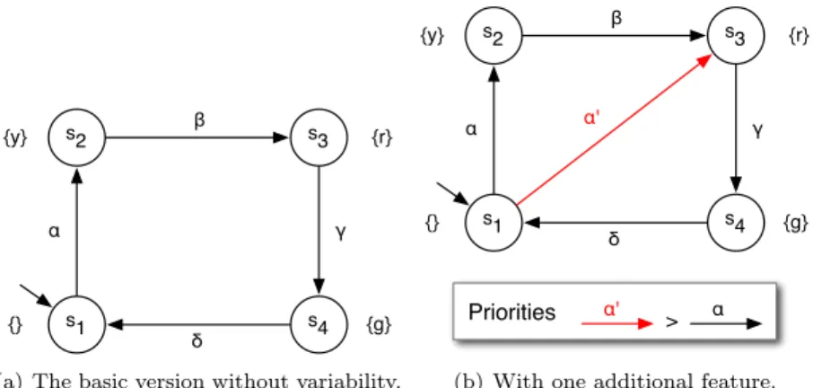
Let us start with the red lights system, a classic among introductory examples in model checking. In its basic version, the red lights controller will switch between

∗_{FNRS Research Fellow.}

(4)

s1 s2 s3 {y} s4 {r} α β γ δ {} {g}

(a) The basic version without variability.

s1 s2 s3 {y} s4 {r} α β γ δ α' {} {g} α Priorities α' _>

(b) With one additional feature.

Figure 1: FTS of the red light controller.

yellow, red and green as shown by the TS in Figure 1(a). Initially the light is off, represented by an empty labelling of the initial state s1; it then switches to yellow in s2(the y label), then to red and then to green. The action names here are not important and were thus named α through δ. So far, the controller can be modelled with a conventional TS.

There exists another version of the controller, which omits the yellow light and immediately shows red. In order to model the second version, one could easily draw a second TS without state s2and a transition from s1to s3—and so forth for every version. In general, however, such an approach would not scale, since the number of different versions can become large. This is despite the fact that these versions generally only differ in small details.

In consequence, we proposed FTS [3], an extension of classical TSs, where transitions can be labelled with features2 _{drawn from a variability model such} as an FD [8]. To model the second red light variant in FTS, it is sufficient to add a transition from s1to s3, to label it with a different feature, say SkipYellow, and to document the fact that there are two variants (one with SkipYellow and one without) in a variability model. The new transition α0 _{also has to be of} higher priority than α, otherwise, the variant with SkipYellow would still have the α transition.

Once an FTS of the system exists, it can be verified using the model checking algorithm proposed in [3]. We focus here on the modelling aspects and will thus not go into details about model checking. In short, it will check a temporal property for all systems represented by the FTS in one shot. In case the property is violated, the algorithm will pinpoint the products that violate it.

(5)

3 The vending machine [5]

The vending machine example originally appeared in [5] to illustrate the use of modal transition systems (MTS) to model the behaviour of software product lines. Following [5], the vending machine has a European variant serving tea and coffee as well as an american variant serving coffee and cappuccino. The European version accepts euro coins while the US version accepts dollars; in ad-dition, the US version rings a tone when the beverage is served. Its behaviour is modelled by the MTS shown in Figure 2. In an MTS, transitions can be optional (represented by dashed lines), which means that MTS, just as FTS, model a set of different TS. For MTS, these can be obtained by removing cer-tain optional transitions and making the others mandatory. For instance, the European variant can be obtained by removing transitions 1$, cappuccino and ring a tone.

Definition 4.1 (Alternative def. MTS) A MTS is a quintu-ple (BS, DS, s0, Act, →) such that (BS ∪ DS, s0, Act, →)

is a LTS and BS ∩ DS = ∅. A MTS has two distinct sets of states: the box states BS and the diamond states DS.

At this point, we define the characteristic formula FC(M) of a (simple) MTS M = (BS, DS, s0, Act, →) as FC(s0), where FC(s) =    ($iPw(αi)) ∧ ((%i[αi]FC(si)) if s ∈ DS (%_iO(αi)) ∧ ((%i[αi]FC(si)) if s ∈ BS

and ∀i: s→ sei iwith I(αi) = {ei}

If we define the characteristic formula in an equational form using the expressions above, we obtain one equation for each state of the MTS, and the equations have a number of terms equal to two times the number of transitions leaving the relevant state. An attempt to write a single characteristic formula gives a formula exponential in size with respect to the number of states, and needs some form of fixed point expression for expressing cycles in the MTS (see [12]).

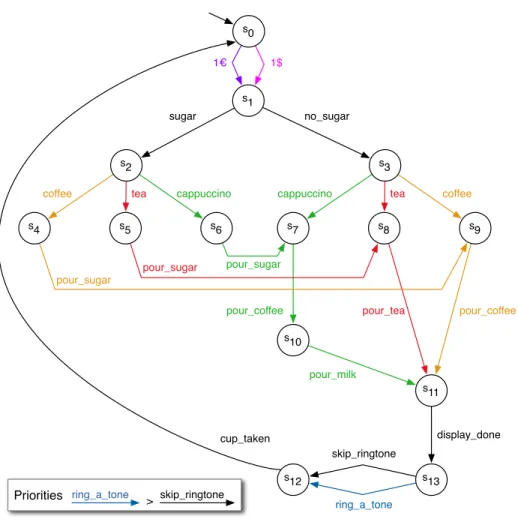
Figure 1. A MTS modeling a product family.

5 An example

Let us consider the example introduced in [8], that is, a family of coffee machines represented by the MTS depicted in Fig. 1, which allows products to differ for the two differ-ent currencies accepted, for the three drinks delivered and for the presence of a ring tone after delivery. In the figure,

solid arcs are required transitions and dashed arcs are possi-ble transitions, that is, states with outgoing solid arcs belong to BS, and states with outgoing dashed arcs belong to DS. The characteristic formula in equational form is given by the following set of equations:

φ0 = (Pw(1e) ∨ Pw(1$)) ∧ ([1e]φ1∧ [1$]φ1)

φ1 = (O(sugar) ∧ O(no_sugar))

∧ ([sugar]φ2∧ [no_sugar]φ3)

φ2 = (Pw(coffee) ∨ Pw(cappuccino) ∨ Pw(tea))

∧ ([coffee]φ4∧ [cappuccino]φ5∧ [tea]φ6)

φ3 = (Pw(coffee) ∨ Pw(cappuccino) ∨ Pw(tea))

∧ ([coffee]φ7∧ [cappuccino]φ8∧ [tea]φ9)

φ4 = O(pour_sugar) ∧ [pour_sugar]φ7 φ5 = O(pour_sugar) ∧ [pour_sugar]φ8 φ6 = O(pour_sugar) ∧ [pour_sugar]φ9 φ7 = O(pour_coffee) ∧ [pour_coffee]φ10 φ8 = O(pour_tea) ∧ [pour_tea]φ11 φ9 = O(pour_coffee) ∧ [pour_coffee]φ11 φ10 = O(pour_milk) ∧ [pour_milk]φ11 φ11 = O(display_done) ∧ [display_done]φ12 φ12 = (Pw(cup_taken) ∨ Pw(ring_a_tone)) ∧ ([cup_taken]φ0∧ [ring_a_tone]φ13) φ13 = O(cup_taken) ∧ [cup_taken]φ0

Note that the characteristic formula given above does not allow, from any state of the considered MTS, to derive a LTS such that the corresponding state has no outgoing tran-sitions, even in the case of diamond states.

The characteristic formula of a MTS implies any other property which is satisfied by the MTS, and can thus serve as a basis for the logical verification over MTSs. Actually, this approach is not as efficient as model-checking ones, but the definition of the characteristic formula may serve as a basis for a deeper study of the application of deontic logics to the verification of properties of families of products.

We now show two exemplary formulae that use deontic operators to formalize properties of the products derived by the family of coffee machines represented by the MTS de-picted in Fig. 1.

1. The family permits to derive a product in which it is permitted to get a coffee with 1e:

Pw(1e) =⇒ [1e] E (tt U Pw(coffee))

2. The family obliges every product to provide the possi-bility to ask for sugar:

A (tt U O(sugar))

VaMoS'09

Figure 2: The vending machine MTS, taken from [5].

However, with the MTS given in Figure 2, it is possible to obtain many more variants. For instance, it is possible to obtain a machine which takes euro coins and rings a tone when a beverage is served. This would correspond neither to the US nor to the European version; still, it can be easily imagined as a valid system. Moreover, it is also possible to obtain a machine that serves coffee always with sugar, and tea and cappuccino always without; or a machine which would accept dollar and euro coins. These systems are probably not among the systems that the engineer had in mind. The problem that we try to illustrate

(6)

coffee tea cappuccino display_done 1€ ring_a_tone s0 s2 s5 s4 s6 s12 s13 tea s3 s8 s7 s9 s1 1$ sugar no_sugar s10 s11 cappuccino coffee pour_sugar pour_sugar pour_sugar pour_tea pour_coffee pour_coffee pour_milk skip_ringtone cup_taken skip_ringtone Priorities ring_a_tone _>

Figure 3: The vending machine modelled as an FTS. VendingMachine v Tea t RingTone t Cappuccino ca Coffee co Beverages bev Currency cur US Dollar usd Euro eur

Legend: a = And a = Or a = Xor

(7)

here is that in MTS, it is not easily possible to model transitions that belong together so that they always appear together in a system, or not at all (such as the two cappuccino transitions in Figure 2).

The vending machine modelled with an FTS is shown in Figure 3. The FD that comes with the FTS is shown in Figure 4. Valid products of the FD are the US and the European version as described above, but also other variants. In contrast to the MTS of Figure 2, the FTS only models systems that are valid, that is: the pairs of coffee, tea or cappuccino transitions always appear together, because they belong to the same feature. Similarly, the machine will either accept dollars or euros, but not both, since the are modelled as alternatives in the related FD.

4 The wiper system [6]

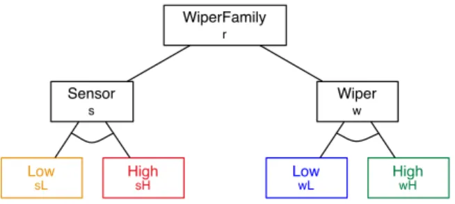
The car wiper system example was proposed by Gruler et al. in [6]. It consists of two subsystems: a sensor unit, able to detect rain, and the wiper itself. Both the sensor and the wiper come in two qualities, high and low. A low quality rain sensor can only distinguish between rain and no rain, whereas the high quality sensor can also discriminate between heavy and little rain. Similarly, the high quality wipers can operate at two speeds, whereas the low quality wiper only operates at one speed. In addition, the low quality wipers can be set to wipe permanently. The FD in Figure 5 models this situation.

WiperFamily r High sH Wiper w Low sL Sensor s High wH Low wL

Figure 5: The FD for the original wiper system.

Gruler et al. propose PL-CCS [6], a variant of CCS where a new operator ⊕ was added to represent alternative choice between two processes. The whole wiper system is modelled with the PL-CCS expression W ipF am in Figure 6, i.e. the parallel composition of the sensor and the wiper subsystem. The sensor subsystem is defined as being either the low or the high quality sensor subsystem. The wiper subsystem is defined similarly.

The PL-CCS definition of the two sensor subsystems is given in Figure 7. The low quality sensor will either sense no rain, or it will sense heavy/little rain in which case it sends the message Rain. As expected, the high quality sensor behaves differently: in case of heavy rain it sends the message HvyRain. An

(8)

4 Specification and Verification of a Sample Product-Line

Let us now demonstrate our approach on a simplified version of an industrial case study we have been working on. We consider a product line whose configurations realize different versions of a windscreen wiper system.

Specification At first, we specify the family of systems, using the formalism introduced

in Section 2. The windscreen wiper systems that we specify in our familyWipFam are each built of two subcomponents: a rain sensor,Sensor, and a windscreen wiper, Wiper. Both subcomponents can be realized by two variants, a high and a low one, respectively:

WipFam def

= Sensor ! Wiper (E1)

Sensor def

= SensL ⊕1SensH (E2)

Wiper def

= WipL ⊕2WipH (E3)

The low variantSensL of the sensor is specified as follows: SensL def

= non.SensL + ltl.Raining + hvy.Raining + noRain.SensL (E4) Raining def

= non.SensL + ltl.Raining + hvy.Raining + rain.Raining (E5) The low variantSensL only detects two different environmental conditions—dry and raining—even though the environment can stimulate the sensor with three differ-ent conditions: hvy for heavy rain, ltl for little rain and non for no rain. However, this sensor cannot differ between heavy and little rain, i. e. for this sensor,hvy and ltl have the same effect, as the sensor reaches a processRaining and provides an action rain, indicating solely the fact that it is raining (without precisely characterizing the intensity). As long as no rain has been detected, the sensor provides the actionnoRain, respectively.

The high version of the sensor can distinguish between different degrees of rain intensity, i. e.SensH additionally differentiates heavy rain from little rain. Its PL-CCS specification is given in the following:

SensH def

= non.SensH + ltl.Medium + hvy.Heavy + noRain.SensH (E6) Medium def

= non.SensH + ltl.Medium + hvy.Heavy + rain.Medium (E7) Heavy def

= non.SensH + ltl.Medium + hvy.Heavy + hvyRain.Heavy (E8) In this product line, the sensors can be arbitrarily combined with two variants of windscreen wipers,WipL and WipH . In particular, for this example we have no addi-tional non-funcaddi-tional dependencies between the possible variants which would restrict the set of combinatorially possible configurations.

The low versionWipL offers two operation modes: (i) a manual mode with perpet-ual wiper arm movement (actionpermWip), which has to be activated explicitly by the

16

Figure 6: The wiper system in PL-CCS, taken from [6].

Low quality.

4 Specification and Verification of a Sample Product-Line

WipFam def

Sensor def

Wiper def

SensH def

16 High quality.

4 Specification and Verification of a Sample Product-Line

WipFam def

Sensor def

Wiper def

SensH def

16

Figure 7: The sensor subsystem in PL-CCS, taken from [6].

s1 s2 s3 non noRain heavy little non non heavy little heavyRain rain heavy little heavy heavy

(9)

Low quality.

driver, (ii) and a semi-automatic interval mode in which the wiper arm moves at a lower frequency triggered by the rain sensor (via the actionrain).

WipL def

= off .WipL + manualOn.Permanent + intvOn.Interval (E9) Interval def

= noRain.Interval + intvOff .WipL + intvOn.Interval (E10) + rain.Wiping + hvyRain.Wiping

Wiping def

= slowWip.Interval + intvOn.Interval (E11) Permanent def

= permWip.Permanent + off .WipL + intvOn.Interval (E12) The high variantWipH can operate at two speeds: slow (action: slowWip) and fast (action:fastWip). Here, the wiper arm movement is fully controlled by the rain sensor and adjusts its frequency automatically to the current rain intensity.

WipH def

= off .WipH + intvOn.AutoIntv (E13) AutoIntv def

= noRain.AutoIntv + intvOn.AutoIntv + rain.Slow (E14) + intvOff .WipH + hvyRain.Fast

Slow def

= slowWip.AutoIntv + intvOn.AutoIntv (E15) Fast def

= fastWip.AutoIntv + intvOn.AutoIntv (E16) The PL-CCS program specifying the entire product lineWipFam is given by the equations E1–E16. The whole programWipFam is well-formed, which allows a unique numbering of all (two) variation points as shown by Equations E2 and E3.

Verification From our example system familyWipFam, we can derive four different

individual systems, as we can combine the subsystem variants arbitrarily. Having spec-ified the family in PL-CCS, we can now apply the model checking approach described in Section 3, in order to verify functional properties for configurations in the system family.

Thinking of a relevant property, for instance, one could possibly be interested in verifying for a windscreen wiping system whether or not a driver is always able to switch to automatic windscreen wiping mode. (Property 1, formalized in Equation 14). Another property could demand the windscreen wiper to wipe fast, once it is raining heavily (Property 2, formalized in Equation 15).

µX.!."X ∨ !intvOn"true (14) νY.[.]Y ∧ (¬!intvOff "true ∨ [hvy]!fastWip"true) (15) In our example, Property 1 holds for the set of all possible configurations!L, L", !R, L", !L, R" ,and !R, R", which can be denoted by the single vector !?, ?". However, Property 2 is only satisfied in the configuration, in which the high variants of both subsystems are used, i. e. the result of applying the proposed model checking algorithm is the set containing the single configuration vector!R, R". Intuitively, it is easy to see why: As the low version of the windscreen wiper does not provide a fast wiping mode, it never provides the output actionfastWip. In consequence, the wind screen wiper can never wipe fast if the low version is used. However, even if the high version of

High quality.

driver, (ii) and a semi-automatic interval mode in which the wiper arm moves at a lower frequency triggered by the rain sensor (via the actionrain).

WipL def

= off .WipL + manualOn.Permanent + intvOn.Interval (E9) Interval def

= noRain.Interval + intvOff .WipL + intvOn.Interval (E10) + rain.Wiping + hvyRain.Wiping

Wiping def

= slowWip.Interval + intvOn.Interval (E11) Permanent def

= permWip.Permanent + off .WipL + intvOn.Interval (E12) The high variantWipH can operate at two speeds: slow (action: slowWip) and fast (action:fastWip). Here, the wiper arm movement is fully controlled by the rain sensor and adjusts its frequency automatically to the current rain intensity.

WipH def

= off .WipH + intvOn.AutoIntv (E13) AutoIntv def

= noRain.AutoIntv + intvOn.AutoIntv + rain.Slow (E14) + intvOff .WipH + hvyRain.Fast

Slow def

= slowWip.AutoIntv + intvOn.AutoIntv (E15) Fast def

= fastWip.AutoIntv + intvOn.AutoIntv (E16) The PL-CCS program specifying the entire product lineWipFam is given by the equations E1–E16. The whole programWipFam is well-formed, which allows a unique numbering of all (two) variation points as shown by Equations E2 and E3.

Verification From our example system familyWipFam, we can derive four different

individual systems, as we can combine the subsystem variants arbitrarily. Having spec-ified the family in PL-CCS, we can now apply the model checking approach described in Section 3, in order to verify functional properties for configurations in the system family.

Thinking of a relevant property, for instance, one could possibly be interested in verifying for a windscreen wiping system whether or not a driver is always able to switch to automatic windscreen wiping mode. (Property 1, formalized in Equation 14). Another property could demand the windscreen wiper to wipe fast, once it is raining heavily (Property 2, formalized in Equation 15).

µX.!."X ∨ !intvOn"true (14) νY.[.]Y ∧ (¬!intvOff "true ∨ [hvy]!fastWip"true) (15) In our example, Property 1 holds for the set of all possible configurations!L, L", !R, L", !L, R" ,and !R, R", which can be denoted by the single vector !?, ?". However, Property 2 is only satisfied in the configuration, in which the high variants of both subsystems are used, i. e. the result of applying the proposed model checking algorithm is the set containing the single configuration vector!R, R". Intuitively, it is easy to see why: As the low version of the windscreen wiper does not provide a fast wiping mode, it never provides the output actionfastWip. In consequence, the wind screen wiper can never wipe fast if the low version is used. However, even if the high version of

17

Figure 9: The wiper subsystem in PL-CCS, taken from [6].

s5 heavyRain intvOn, fastWipe s4 rain intvOn, slowWipe s1 s2 s3 off intvOn off intvOff intvOn noRain permWipe intvOn manualOn heavyRain

(10)

immediate observation is that both subsystems are quite similar and that the sending of the Rain message is the same in both cases. Still, the corresponding part has to be duplicated inside both subsystems. An equivalent description in FTS is given in Figure 8. Since the part dealing with the detection of little or no rain is the same for both qualities, the corresponding actions in the FTS are part of the base system instead of being duplicated. Both features visibly differ only in the handling of the heavy rain condition. Note that in Figure 8 and subsequent figures, labels in bold font denote transitions which are synchronised in a parallel composition.

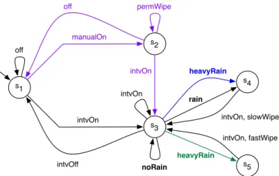
As of the two wiper subsystems, their PL-CCS definition is given in Figure 9. Both subsystems have an interval switch, which will switch interval wiping on. During interval wiping, both subsystems wipe if the sensor subsystem reports rain; the high quality subsystem will wipe faster in case of heavy rain. In ad-dition, the low quality wiper can be set to permanent wiping, which ignores the rain sensor. Here again, both subsystems are almost identical (except for the permanent wiping function), the sole difference being that the high qual-ity variant reacts differently to a HvyRain message. As a consequence, the definitions for both subsystems are almost duplicates. This duplication is not needed in FTS. Consider the FTS representation of the wiper subsystem shown in Figure 10. It clearly shows that (except for the permanent wiping function) both versions only differ in their handling of HeavyRain.

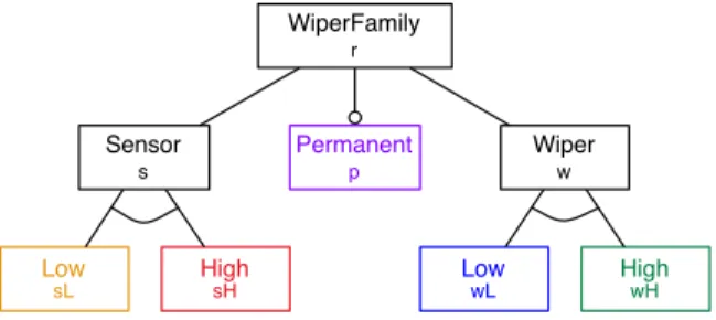
We conclude this example with an extension that is not part of the original paper [6]. Consider the case in which the permanent wiping feature can also be supported by high quality wipers (in fact, there is no reason why it should not). That is, permanent wiping will become an individual feature which is optional. A revised FD that accommodates the new feature is presented in Figure 11. To make the corresponding change in the behavioural model, in FTS it is sufficient to relabel the transitions pertaining to the wiping feature, as shown in Figure 12. In PL-CCS, on the other hand, one will have to duplicate the definition of the permanent wiping mode in both subsystem definitions.

WiperFamily r High sH Wiper w Low sL Sensor s High wH Low wL Permanent p

Figure 11: A FD for the wiper system in which permanent wiping is explicitly represented as a feature.

(11)

s5 heavyRain intvOn, fastWipe s4 rain intvOn, slowWipe s1 s2 s3 off intvOn off intvOff intvOn noRain permWipe intvOn manualOn heavyRain

Figure 12: The modified FTS for the wiper system with permanent wiping as a separate feature.

5 The mine pump system [7]

The purpose of the mine pump system [7] is to keep a mine shaft clear of water while avoiding the danger of a methane related explosion. It consists of a water pump, a sensor measuring the water level and a sensor measuring the abundance of methane in the mine. The system is supposed to activate the pump once the water level reaches a preset threshold, but only if the methane is below a critical limit. MinePumpSys base Methane detect. m Command c Water regulation l

Figure 13: An initial FD for the mine pump controller.

The system consists of three high-level features, shown in Figure 13: (i) a command interface c, which can be used to switch the water regulation function on or off; (ii) a methane alarm interface m, which can receive alarm messages from the methane sensor in case of critical methane, and (iii) the water regula-tion subsystem l. The system is modelled by the FTS in Figure 14. It maintains a variable representing the system state, and its reactions to events such as a methane alarm or high water depend on this state. In order to keep the de-scription intuitive, the system state is modelled in a separate FTS, shown in Figure 15. Basically, the main FTS only describes the actions on the system

(12)

s 6 s 7 commandMsg s 8 receiveMsg s 9 stopCmd s13 startCmd s10 isRunning isNotRunning s11 pumpStop s14 isRunning isReady isNotRunning s15 setReady s16 s17 isRunning isNotRunning s18 palarmMsg s12 setStop pumpStop s19 setMethaneStop levelMsg s20 s21 highLevel lowLevel normalLevel s22 isReady _isLowStop s23 setReady setMethaneStop s24 isReady s25 pumpStart _isNotReady s26 setRunning isRunning isStopped isMethaneStop s27 s28 isRunning isNotRunning s29 pumpStop s30 setLowStop {start} {msg} {command} {stopcommand} {startcommand} {palarm} {level}

(13)

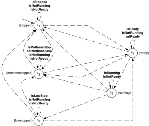
state, but does not record it explicitly. The actual FTS of the controller is the parallel composition of these two FTS. Note that in Figure 15 and subse-quent figures, transitions represented by dashed lines are transitions that are not labelled by a feature. These transitions will be synchronised during par-allel composition and take the feature of the transition with which they are synchronised. s5 s1 s4 isRunning isNotReady isReady isNotRunning setReady isStopped isNotRunning isNotReady s2 isMethaneStop setMethaneStop isNotRunning isNotReady s3 isLowStop isNotRunning isNotReady {stopped} {methanestopped} {lowstopped} {ready} {running}

Figure 15: The FTS modelling the system state. The transitions between states are implicitly named setNewState where NewState is the name of the state in which the transition arrives, e.g. setReady.

Intuitively, each time the main FTS executes a set* action, e.g. setReady, it will be synchronised with the corresponding transition in the state FTS. The result is that the state in which the transition arrives is labelled with the new state, e.g. ready. The state FTS will thus add an atomic proposition with the system state to each state of the main FTS. This causes a small blowup; the resulting FTS will have hundreds of states.

There are five system states:

• stopped means that the water regulation function is off (controlled via the command interface). The system will in no case switch the pump on.

(14)

• ready means that the water regulation function is on (controlled via the command interface). The system will switch the pump on if there is no methane and the water level is high.

• running means that the pump is currently running.

• lowstopped means that the pump was stopped because the water level was low. The pump will resume in case the water rises again.

• methanestopped means that the pump was stopped because of a critical methane level. The pump will not resume until explicitly told so via the command interface.

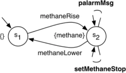
The system operates as follows. It will observe three types of events: com-mands, methane alarm messages and water readings. There are two types of command: stop and start. In case of a start command, the system state is changed and set to ready. In case of a stop command, the pump is stopped, and the system state set to stopped. In case of a methane alarm, the system stops the pump and sets the system state to methanestopped. The system can distinguish between three different water levels: in case of normal water, the system does nothing; if the water is high and the pump not yet running, the system will first check whether it is ready or whether it just stopped because of low water (lowstopped), if yes, it will check the methane level, and if there is no methane (that is, if after the check it is still ready), it will start the pump and set the state to running, otherwise it will do nothing. Once the water is low, the system switches off the pump and sets the system state to lowstopped. The system interacts with its environment, which is modelled with three other FTS that are put in parallel with the FTS of the system. The methane level is modelled with the FTS in Figure 16. Methane can rise and lower at will, represented by the methaneRise and methaneLower transitions. The pAlarmMsg and setMethaneStop transitions will synchronise with the system FTS, meaning that the system FTS will receive the alarm message only in case of high methane. The water pump is represented by the FTS in Figure 17. The pump can be in two states, running or stopped, and the actions pumpStart and pumpStop, synchronised with the system FTS, will cause this state to change. The action pumpRunningis used to model the interaction between the pump and the water. It is synchronised with the water FTS shown in Figure 18: a running pump will

s2 palarmMsg s1 methaneRise methaneLower setMethaneStop {} {methane}

(15)

s2 pumpRunning s1 pumpStart pumpStop {pumpoff} {pumon}

Figure 17: An FTS modelling the environment: the pump.

s3 highLevel s1 normalLevel s2 lowLevel waterRise waterRise pumpRunning pumpRunning pumpRunning

{lowwater} {normalwater} {highwater}

Figure 18: An FTS modelling the environment: the water level. cause the water level to decrease. The level can rise at will. The low, high and normalLevel actions are synchronised with the main FTS, meaning the system will only observe low, high or normal water if this is indeed the case.

When the command interface and the methane alarm interface are considered optional, as in the first FD in Figure 13, there are four different products. We can add further variability by considering the start and stop message types as well as the three water level readings as individual features. A revised FD is shown in Figure 19. The product line now has 64 products. The revised system FTS is given in Figure 20. The other FTS do not change. Please refer to [3] for a list of LTL properties that were checked for these two FTS as a benchmark of the performance of our model checking procedure.

MinePumpSys base Methane detect. m Command c Water regulation l Stop cp Start

ct Lowll Normalln Highlh

(16)

s 6 s 7 commandMsg s 8 receiveMsg s 9 stopCmd s13 startCmd s10 isRunning isNotRunning s11 pumpStop s14 isRunning isReady isNotRunning s15 setReady s16 s17 isRunning isNotRunning s18 palarmMsg s12 setStop pumpStop s19 setMethaneStop levelMsg s20 s21 highLevel lowLevel normalLevel s22 isReady _isLowStop s23 setReady setMethaneStop s24 isReady s25 pumpStart _isNotReady s26 setRunning isRunning isStopped isMethaneStop s27 s28 isRunning isNotRunning s29 pumpStop s30 setLowStop {start} {msg} {command} {stopcommand} {startcommand} {palarm} {level}

(17)

References

[1] C. Baier and J.-P. Katoen. Principles of Model Checking. MIT Press, 2007. [2] E. Clarke, O. Grumberg, and D. Peled. Model Checking. MIT Press, 1999. [3] A. Classen, P. Heymans, P.-Y. Schobbens, A. Legay, and J.-F. Raskin. Model

checking lots of systems: Efficient verification of temporal properties in soft-ware product lines. In 32nd International Conference on Softsoft-ware Engi-neering, ICSE 2010, May 2-8, 2010, Cape Town, South Africa, Proceedings. IEEE, 2010. To appear.

[4] P. C. Clements and L. Northrop. Software Product Lines: Practices and Patterns. SEI Series in Software Engineering. Addison-Wesley, August 2001. [5] A. Fantechi and S. Gnesi. Formal modeling for product families engineering.

In SPLC 2008, pages 193–202. IEEE CS, 2008.

[6] A. Gruler, M. Leucker, and K. Scheidemann. Modeling and model checking software product lines. In IFIP WG 6.1 FMOODS ’08, pages 113–131. Springer, 2008.

[7] J. Kramer, J. Magee, M. Sloman, and A. Lister. Conic: an integrated approach to distributed computer control systems. Computers and Digital Techniques, IEE Proceedings E, 130(1):1–10, 1983.

[8] P.-Y. Schobbens, P. Heymans, J.-C. Trigaux, and Y. Bontemps. Feature Diagrams: A Survey and A Formal Semantics. In RE’06, pages 139–148, 2006.